Qui ci stanno le dediche. Con LAT EX 2ε bisogna mettere un doppio backslash \\ per andare a capo. Indice Sommario I vii Formattazione in ambiente LATEX 2ε e Office 1 Misure standard 1.1 Impaginazione . . . . . . . . . . . . . . . . . . . . . . . . . . . . . . . 1.2 1.3 1 3 3 Misure della carta e dei margini . . . . . . . . . . . . . . . . . . . . . Caratteri . . . . . . . . . . . . . . . . . . . . . . . . . . . . . . . . . . 5 6 1.3.1 Font e dimensioni . . . . . . . . . . . . . . . . . . . . . . . . . 6 1.4 1.3.2 Elenchi ed indice . . . . . . . . . . . . . . . . . . . . . . . . . Le tabelle . . . . . . . . . . . . . . . . . . . . . . . . . . . . . . . . . 8 9 1.5 Le figure . . . . . . . . . . . . . . . . . . . . . . . . . . . . . . . . . . 9 1.6 1.7 La bibliografia . . . . . . . . . . . . . . . . . . . . . . . . . . . . . . . Le equazioni . . . . . . . . . . . . . . . . . . . . . . . . . . . . . . . . 10 11 1.8 Stampa . . . . . . . . . . . . . . . . . . . . . . . . . . . . . . . . . . 12 2 Alcuni suggerimenti per i LATEXatori 13 2.1 Preambolo . . . . . . . . . . . . . . . . . . . . . . . . . . . . . . . . . 14 2.2 2.3 Titolo . . . . . . . . . . . . . . . . . . . . . . . . . . . . . . . . . . . Copy e dediche . . . . . . . . . . . . . . . . . . . . . . . . . . . . . . 15 15 2.4 2.5 Indice, Elenchi e Sommario . . . . . . . . . . . . . . . . . . . . . . . . Capitoli, sezioni ecc. . . . . . . . . . . . . . . . . . . . . . . . . . . . 15 15 2.6 Bibliografia . . . . . . . . . . . . . . . . . . . . . . . . . . . . . . . . 16 2.7 DVI, PS e PDF (stampa) . . . . . . . . . . . . . . . . . . . . . . . . . 16 i ii Indice II Esempio preso da un articolo 19 3 First evidence of post-seismic deformation in the central Mediterranean: Crustal viscoelastic relaxation in the area of the 1980 Irpinia earthquake (Southern Italy) 3.1 abstract . . . . . . . . . . . . . . . . . . . . . . . . . . . . . . . . . . 3.2 Introduction . . . . . . . . . . . . . . . . . . . . . . . . . . . . . . . . 3.3 The viscoelastic deformation model and earthquake parameters . . . . . 3.4 Modeling results . . . . . . . . . . . . . . . . . . . . . . . . . . . . . 3.5 Discussion and conclusions . . . . . . . . . . . . . . . . . . . . . . . . 3.6 acknowledgments . . . . . . . . . . . . . . . . . . . . . . . . . . . . . 21 21 22 23 25 29 30 A Questa è una appendice A.1 Da un articolo. . . . . . . . . . . . . . . . . . . . . . . . . . . . . . . . 31 31 Ringraziamenti 33 Bibliografia 35 Elenco delle figure 1.1 1.2 Logo Unimi . . . . . . . . . . . . . . . . . . . . . . . . . . . . . . . . Logo Scuola . . . . . . . . . . . . . . . . . . . . . . . . . . . . . . . . 10 11 3.1 3.2 3.3 3.4 Faulted area . . . Levelling . . . . Modelling results Model results . . 24 25 27 29 . . . . . . . . . . . . . . . . . . . . . . . . . . . . . . . . . . . . iii . . . . . . . . . . . . . . . . . . . . . . . . . . . . . . . . . . . . . . . . . . . . . . . . . . . . . . . . . . . . . . . . . . . . . . . . . . . . . . . . Elenco delle tabelle 1.1 Caratteristiche ambienti . . . . . . . . . . . . . . . . . . . . . . . . . . 9 3.1 3.2 3.3 Viscoelastic parameters . . . . . . . . . . . . . . . . . . . . . . . . . . Fault elements . . . . . . . . . . . . . . . . . . . . . . . . . . . . . . . Seismic distribution . . . . . . . . . . . . . . . . . . . . . . . . . . . . 23 25 26 v Sommario Questa mini guida è destinata agli utenti LATEX 2ε come modello per la tesi di dottorato. Tuttavia, indica anche agli utenti (Open)Office la base di lavoro e formattazione comune. Il primo capitolo indicherà le misure comuni, il secondo invece sarà destinato principalmente agli utenti LATEX per la descrizione di alcuni comandi/accorgimenti. Nel poco tempo che ho avuto a disposizione, questo é quanto di meglio sia riuscito a fare. Spero possiate comunque apprezzare lo sforzo, e che questo vi aiuti nella stesura della tesi. Buon lavoro! Giorgio vii Parte I Formattazione in ambiente LATEX 2ε e Office 1 Capitolo 1 Misure standard In questo capitolo troveremo le misure standard usate per la costruzione di questo libretto, che poi saranno quelle della tesi. Per gli utenti LATEX 2ε non dovrebbero esserci problemi, tanto decide tutto il sistema dato il modello; per gli utenti Office, invece, sono dati essenziali in quanto non ho fatto in tempo a fare in modello .dot per loro (scusate...) Per gli utenti Office verranno di seguito indicate le convenzioni chiave da impostare. Quello che non troverete indicato, cercate di estrapolarlo quanto meglio potete con il righello (!) da questo file pdf, per uniformarsi alle convenzioni LATEX. Per avere una idea precisa delle dimensioni, questo pdf è fatto in modo da avere i segni di ritaglio per il formato “libretto” e deve essere stampato SENZA essere riscalato. . . . Non infierite su di me per eventuali errori di grammatica o di sintassi o incomprensibilità del testo, sono le 2 di notte e sto schiattando dal sonno... In caso di dubbi, scrivetemi una e-mail a [email protected] o contattatemi per telefono allo 02 503 18471. 1.1 Impaginazione Il FRONTESPIZIO della tesi e la tesi vera e propria sono due cose diverse. Il Frontespizio sarà fornito come file doc di modello per gli utenti Office e ci sarà il file frontespizio.tex come documento separato nel pacchetto per gli utenti TEX. Per quanto riguarda la tesi propriamente detta, essa è così composta: 3 4 1. Misure standard 1. Pagina di titolo (per ora provvisoria, in via di definizione), destra∗ 2. Pagina copyright (forse a cura della stamperia), sinistra 3. Pagina di dedica (alla mia morosa...), senza numero di pagina, destra 4. Pagina BIANCA (senza numero) per fare iniziare l’indice a destra 5. Indice, prima pagina a destra (in cui inizia la numerazione romana, partendo da i) 6. eventuale PAGINA BIANCA per far iniziare l’elenco delle figure a destra 7. (Facoltativo) Elenco delle figure, prima pagina a destra (continua la numerazione romana) 8. eventuale PAGINA BIANCA per far iniziare l’elenco delle tabelle a destra 9. (Facoltativo) Elenco delle tabelle, prima pagina a destra (continua la numerazione romana) 10. eventuale PAGINA BIANCA per far iniziare il sommario a destra 11. Sommario, prima pagina a destra (continua la numerazione romana) 12. eventuale PAGINA BIANCA per far iniziare il capitolo a destra 13. da qui in poi ci sono i CAPITOLI. dalla prima pagina del primo capitolo parte la numerazione araba (1, 2, 3. . . ). I capitoli iniziano sempre sulla destra, quindi nel caso aggiungere una pagina vuota fra un capitolo e l’altro per compensare. 14. dopo tutti i capitoli ci vanno i RINGRAZIAMENTI e la BIBLIOGRAFIA, entrambi aprono su pagina destra (inserire eventualmente pagina vuota) e continuano la numerazione dei capitoli. Tralasciando le parti con numerazione romana, dall’inizio dei capitoli le pagine DISPARI sono pagine DESTRE (quindi tutti i capitoli aprono su pagina destra che e’ dispari, a partire dal primo che inizia a pagina 1). ∗ Per pagina destra si intende una pagina che è a destra della legatura e ha il bordo destro libero. Pagina sinistra e’ invece l’opposto. . . Questa fra le altre cose è un buon esempio di nota a piè di pagina 1.2 Misure della carta e dei margini 5 Le prime pagine di indice, elenchi, sommario, capitoli, ringraziamenti e bibliografia NON HANNO intestazione ed i numeri delle pagine vanno a piè di pagina, centrati; per le restanti pagine, tutte le informazioni si trovano in intestazione; l’intestazione è formata da una linea larga 0.3pt, lunga tutta la lunghezza coperta dal testo (vedi sezione sui margini), posta a 20mm dal bordo superiore del foglio, sopra la quale vi è il testo cosí definito: Pagine pari , cioé sinistre, hanno allineato a sinistra il numero di pagina e allineato a destra il numero del capitolo ed il titolo (anche breve) del capitolo, separati da un punto (es. 1. Introduzione); eventualmente vedere come è fatto su questo manualetto. Pagine dispari , cioé destre, hanno allineato a destra il numero di pagina e allineato a sinistra il numero del capitolo, della sezione ed il titolo (anche breve) della sezione, i due numeri separati da un punto mentre il titolo da uno spazio (es. 1.2 Impostazioni generali). 1.2 Misure della carta e dei margini Il formato della carta é il formato “libretto” corrispondente alle dimensioni 170mm x 240mm. Per gli utenti Office, impostare a queste dimensioni il foglio come impostazioni personalizzate dovrebbe garantire che avvenga solo un eventuale riscalamento minimo in fase di stampa della copisteria e questo ci basta. A causa dalla rilegatura, ovviamente parte del margine interno sará dedicato a questa. Si sono tarati i margini interno ed esterno in modo che, una volta tolta la parte di margine destinata alla rilegatura, fra i testi delle due pagine affiancate vi sia (circa) lo stesso spazio deputato ai due margini esterni, quindi: margine interno 15mm dal bordo interno margine esterno 20mm dal bordo esterno limite superiore del corpo del testo 25mm dal bordo superiore limite inferiore del corpo del testo 25mm dal bordo inferiore 6 1. Misure standard inizio del piè di pagina: il piè di pagina inizia appena al di sotto del limite inferiore del corpo del testo e contiene soltanto i numeri di pagina (quando sono a piè di pagina). Ricordo che le note a piè di pagina stanno dentro al corpo del testo; il testo regolare dovrà quindi alzarsi fino a quantoo necessario per far loro posto. Le linee nell’intestazione vanno dal margine sinistro a quello destro, per tutta la larghezza del testo del corpo (135mm). Nel caso rimanga questo stile di titolo, anche le linee orizzontali nel titolo hanno questa lunghezza (fare conto che il titolo è una pagina destra. . . ). 1.3 Caratteri I due set principali di caratteri sono il Times od il Bookman per quanto riguarda i caratteri Serif ed il Helvetica per quanto riguarda i caratteri Sans Serif. Al set Helvetica si puó sostituire anche il set Arial che resta più leggero. Userò nella descrizione le seguenti sigle: it (italics, corsivo), bf (boldface, grassetto), serif (famiglia serif) e sans (famiglia sans serif). L’interlinea di base di tutta la tesi è 1 e 12 , tranne che per la pagina del titolo dove è singola nell’header e 1 e 1 2 nel titolo e footer. Le note a piè di pagina sono ad interlinea singola. 1.3.1 Font e dimensioni partendo dalla pagina del titolo in poi, cercherò ora di specificare tutti i caratteri usati. Sarebbe forse comodo per gli utendi Office fare una copia di questo pdf per poi appuntarci sopra le varie specifiche man mano che vengono descritte. L’idea è che si usi il serif per il corpo deel testo ed il sans per i titoli, per distinguere un pó le due cose. Titolo Per il titolo dovremmo fare un modello di frontespizio anche per gli utenti Office. Nel caso non ci riuscissimo, queste sono le linee guida. La famiglia usata nel titolo é interamente un serif, centrato. Cambiano le dimensioni e la tipologia nei vari passi. L’intestazione parte dal margine superiore, seguita a 2mm 1.3 Caratteri 7 dalla linea che va da margine sinistro a margine destro. Il piè di pagina ha come limite inferiore il margine inferiore, ha subito sopra (2mm) la linea. Fra le due linee ci sta il testo del titolo con l’aggiunta Tesi di Dottorato di Ricerca di ed il nome. La disposizione deve essere bilanciata in modo da far restare circa 1 3 dello spazio bianco sopra e 2 3 sotto. Nell’intestazione, a lato delle prime tre righe vanno messi i simboli dell’università e quello della scuola;il primo è alto 17mm e allineato al margine sinistro, il secondo è invece largo 20mm ed allineato al margine destro. Fra le prime 3 righe e le seguenti c’è uno spazio di circa 1cm. Universitá. . . Milano serif 12pt bf Facoltà. . . XVIII serif 12pt. Solo “Ardito Desio” ed il titolo della Scuola sono it interlinea 1 e 1/2 Titolo serif 25pt bf Tesi di Dottorato. . . serif 11pt Nome serif 14pt bf Piè di pagina serif 12pt bf, tranne che per “Tutor” e “Coordinatore” in it Copyright Si deciderá con la tipografia, per ora nulla Dediche Serif 11pt. Ulteriori specifiche non obbligatorie potrebbero essere it allineato a destra o centrato, ma essendo una cosa personale, lasciamo libertà di scelta. . . Indice, elenchi, capitoli, sommario ecc. ecc. Per ciascuno di questi elementi vige la regola che sono tutti considerati come capitoli; la prima pagina ed̀iversa dalle altre, quindi descriviamo le due cose separatamente. Ora diamo i tratti comuni, poi per l’indice e gli elenchi saranno date le specifiche particolari. 8 1. Misure standard Le Prime pagine aprono sempre a destra, il numero della pagina è centrato al footer. Viene lasciato uno spazio libero prima del titolo del capitolo. Le altre pagine hanno in intestazione gli elementi già descritti, in carattere serif 11pt bf. Per quanto riguarda i titoli, vale quanto sotto: Capitolo e numero del capitolo sans 20pt bf titolo capitolo (anche per titolo elenchi, sommario, ecc.) sans 25pt bf sezioni sans 14pt bf sottosezioni sans 12pt bf sotto-sottosezioni sans 11pt bf I capitoli, le sezioni e le sottosezioni sono numerati mentre le sotto-sottosezioni non sono numerate; indice, elenchi, sommario, ringraziamenti e bibliografia sono visti come capitoli senza numero. Didascalie Le didascalie sono sans 8pt, interlinea singola. Tabelle Le tabelle nello stile LATEX sono di default in interlinea singola, serif 11pt. A causa della variabilità delle cose da metterci dentro, ovviamente le cose variano a piacimento. . . . Figure Solo un suggerimento: il testo nelle figure è più leggibile se è una famiglia sans serif (almeno così dicono sui giornali dell’AGU. . . ). 1.3.2 Elenchi ed indice I caratteri dell’indice e degli elenchi sono tutti in 11pt. Per gli elenchi, sono tutti in Serif. Nell’indice invece le cose si complicano: le parti sono in Sans bf 12pt; i capitoli, sommario, ringraziamenti e tutto il resto che e’ sostanzialmente un capitolo hanno carattere 1.4 Le tabelle 9 Sans 11pt bf; fra titolo e pagina non vi è alcun segno di giunzione. Le sezioni e le sottosezioni sono in Serif 11pt e fra titolo e numero di pagina vi è del puntinato. Se non è possibile riprodurre questo stile in Office, fare pure tutto in Serif. In ogni caso prendete spunto da quanto offerto in questo manualetto. 1.4 Le tabelle Per quanto riguarda le tabelle, a causa della varietà impressionante di stili e di necessità, non ci sono particolari disposizioni per il loro formato. Ambiente Indice Elenco tabelle Elenco figure Sommario Capitoli Sezioni Sottosezioni Sotto-sottosezioni Ringraziamenti Bibliografia Numerato Facoltativo * * * * * Tabella 1.1: Alcune caratteristiche degli ambienti di LATEX 2ε usati in questa tesi. Questa è la didascalia lunga cui verrà sostituita in elenco delle figure la didascalia corta. La tabella 1.1 rappresenta una semplice tabella come può essere fatta in LATEX 2ε . Ovviamente è possibile fare tabelle anche più complesse, o più semplici. 1.5 Le figure Per le figure, anche qui c’è poco da dire. Solo un paio di raccomandazioni (per esperienza diretta): usare una risoluzione alta (almeno 600dpi) e non aspettarsi che i colori vengano fuori come sono sul video. . . Non so ancora se useranno stampe in tricromia (RGB) o in quadricromia (CMYK), comunque a meno che tutta la catena (video vostro, stampante vostra, video loro, stampante loro) abbia il profilo cromatico settato esattamente sugli stessi parametri e questi siano ottimali per tutti (cosa praticamente impossi- 10 1. Misure standard bile), anche nel migliore dei casi ci saranno delle differenze. Un esempio di figura puo’ essere: Figura 1.1: Questo è il nuovo logo dell’università, da usare al posto di quello ovale La figura 1.1 è il nuovo logo dell’università; è stato cambiato dopo l’ottantesimo anniversario. Non ce l’hanno in molti e spesso viene usato ancora quello ovale. Lo troverete in questo pacchetto con il nome minerva.tif oppure minerva.eps in funzione del fatto che usiate Office o LATEX, rispettivamente (LATEX 2ε utilizza di default il formato eps). La figura 1.2 è invece il nuovo logo della scuola di dottorato, che troverete anch’esso nel pacchetto con i nomi logo.gif e logo.eps: essendo in bianco e nero, non e’ necessario usare il formato tif. Se avete bisogno di un logo con risoluzione maggiore (ma non credo), potete convertire l’eps alla risoluzione che volete, visto che è in grafica vettoriale. 1.6 La bibliografia Per quanto riguarda la bibliografia, gli utenti Office possono seguire lo stile di questa pubblicazione, cioé: Per un articolo: Riva, R. E. M., and L. L. A. Vermeersen (2002), Approximation method for high-degree harmonics in normal mode modelling, Geophys. J. Int., 151(1), 309–313. Per un libro: Sabadini, R., and L. L. A. Vermeersen (2004), Global dynamics of the Earth. Applica- 1.7 Le equazioni 11 Figura 1.2: Questo è il nuovo logo della scuola di dottorato tions of normal mode relaxation theory to solid-earth geophysics, Modern approaches in geophysics vol. 30, Kluwer Academic Publisher, Boston. Per gli utenti LATEX si può usare sia lo stile bibliografico nativo del pacchetto BIBTEX sia si può fare manualmente come per Office. (come é fatto qui). La citazione nel testo deve però apparire così: tutto fra parentesi (Sabadini & Vermeersen, 2004), più di una referenza (Cattin & al., 1999; Riva & Vermeersen, 2002), oppure personalizzando nel modo seguente, come avviene in Sabadini & Vermeersen (2004), che lascia solo l’anno tra parentesi. 1.7 Le equazioni Anche in questo caso, mi appello al vostro buon senso. Qui sotto riporto qualche esempio, nel caso voleste uniformarvi. Però già sapete che il sistema LATEX2 è mooooolto più avanti di Office in questo campo quindi non insisterò oltre nel girare il coltello nella piaga. . . d y = A · y + f ∗, dr (1.1) f ∗ = f δ(r − rs ) + f ′ δ′ (r − rs ), (1.2) ed ora qualche equazione un pò più pittoresca: 12 1. Misure standard y(r) = ... −1 ′ −1 Y(r)[Y (rs )(I f + A(rs )f ) + Y (b)y(b)] rs ≤ r ≤ a Y(r)Y −1 (b)y(b) (1.3) b ≤ r ≤ rs la matematica può essere anche inserita nel testo come in. . . . Le componenti del tensore delle deformazioni, scritte in funzione della dislocazione ~s = uêr + vêϑ (1.4) . possono essere espresse come: ǫrr = ∂r u ǫϑϑ = r −1 (1.5) (∂ϑ v + u) −1 ǫϕϕ = r (v cot ϑ + u) 1 ǫrϑ = (∂r v − r −1 v + r −1 ∂ϑ u) 2 1.8 (1.6) (1.7) (1.8) Stampa Circa la stampa della tesi, per quanto riguarda gli utenti LATEX 2ε vedere il prossimo capitolo; per gli utenti Office, una volta generata la tesi definitiva, impostando direttamente il formato della pagina a 17x24cm, usate un pdf writer (se ne volete uno, è disponibile freeware al sito www.pdf995.com/download che ve lo porterò in formato pdf pronto per la stampa. A scanso di equivoci, controllate attentamente il pdf, in modo che sia giusto. Solo una nota sul pdfwriter: gra le preferenze fate in modo di selezionare “massima portabilità” per includere tutti i caratteri e di specificare la massima qualità possibile delle immagini. E con questo dichiaro finita la parte rivolta a tutti del modello di tesi. Nel prossimo capitolo tratteremo cose espressamente legate a LATEX. Capitolo 2 Alcuni suggerimenti per i LATEXatori Questo secondo capitolo è per i LATEXatori e contiene alcune descrizioni dei comandi LATEX utilizzati. Inizio con il dire che non si tratta di un .cls originale. . . Ho spiluccato qua e là, preso pezzi a destra e a manca, per arrivare a questo punto. Vi darò di seguito solo qualche dritta, per il resto confido che voi sappiate leggere un testo LATEX, capirlo e prenderne spunto. Il file book1.cls (modificato da book.cls) contiene tutte le modifiche (o quasi) richieste. A causa della richiesta sulle note a piè di pagina a 8pt con corpo del testo a 11pt, ho dovuto ridefinire la footnotesize (che in formato 11pt sarebbe da 9pt) a scriptnotesize (8pt), questo significa che entrambe le misure ora sono 8pt e non esiste un 9pt. Se lo trovate troppo scomodo, siete liberi di commentare quella riga (\global\let\footnotesize\scriptsize) in book1.cls. Il frontespizio è un file a parte che troverete nel pacchetto con il nome frontespizio.tex e risponde alle dimensioni specifiche date da Artioli. Fate conto che, qui come nel titolo della tesi, una volta ottenuta l’immagine finale dellavscuola di dottorato, bisognerà cambiare il nome dell’immagine nell’includegraphics di destra. La tesi propriamente detta parte dalla pagina del titolo e si compila aa partire dal file tesi.tex. Il lavoro è suddiviso per capitoli. In tesi.tex vi sono solo l’input del preambolo, dove sono tutti i comandi specifici e gli include che puntano ai vari capitoli. I file .tex specifici sono, nell’ordine (quelli fondamentali): 13 2. Suggerimenti LATEX 14 1. titolo.tex: il titolo 2. copy.tex: la pagina di copyright 3. dedication.tex: pagina delle dediche 4. elenchi.tex: indice, elenco delle tabelle e delle figure 5. abstract.tex: sommario 6. part1.tex, capitolo1.tex, capitolo2.tex. . . : parti e capitoli (le parti sono opzionali) 7. appendici.tex: capitolo delle appendici, che parte con un comando\appendix; dopo tale comando, ogni nuovo capitolo è considerato appendice 8. acknowledgements.tex: ringraziamenti 9. bibliografia.tex: bibliografia Vediamo ora alcune caratteristiche particolare, file per file. 2.1 Preambolo Il file preamble.tex contiene tutte le informazioni di formattazione, in particolare sono da selezionare la lingua nel caricamento del package babel (italian/english) alla quarta riga del preamble; i \newcommand utilizzati per dare il nome corretto alle varie sezioni in lingua inglese sono già state inseriti/modificati in book.cls; fate conto che sono rimasti un paio di \renewcommand verso la fine del preambolo per specificare alcuni nomi in italiano. In questo file è stata usata la lingua italiana, quindi il preambolo va già bene per una tesi scritta in italiano. Per la lingua inglese va selezionato english in babel, e commentati i due renewcommand per la lingua italiana che si trovano verso il fondo del preambolo \renewcommand{\acknowledgename}{Ringraziamenti} e il \renewcommand{\abstractname}{Sommario}. 2.2 Titolo 2.2 15 Titolo Per quanto riguarda il titolo, (lo stesso vale per il frontespizio) sono stati ridefiniti i campi da personalizzare con dei \renewcommand iniziali, cosicchè una volta definiti questi si adatta il resto della pagina. Nel caso vi sia anche un co-tutore bisogna decommentare sia il renewcommand sia le due righe di comandi che pongono il co-tutor sotto il tutor alla fine della pagina di tesi (i comandi sono verso la fine del file). Vi sono due entry chiamate spaziosopra e spaziosotto da definire, in modo che il titolo abbia rispettivamente 1/3 e 2/3 di spazio libero dalle righe superiore e inferiore, e che il blocco tutore – anno accademico – coordinatore sia quanto piu’ vicino al margine inferiore. Una unica particolarità è che bisogna stare attenti a che il titolo non sia troppo lungo. In questa eventuale funesta ipotesi potete o passare da \Huge a \huge nel corpo del titolo oppure ridurre il titolo! Può aiutare interrompere manualmente il titolo per metterlo su piú righe usando un doppio backslash. 2.3 Copy e dediche Per la pagina di copyright per ora non possiamo fare nulla. Vedremo se fornire alla fine il file copyr.tex definitivo o se lasciare l’onere alla copisteria. Per le dediche, fate voi. Attualmente vige un \flushright per allineare tutto a destra, ma volendo potete anche centrare sostituendo ai due flushright due center (nella definizione ad inizio file). 2.4 Indice, Elenchi e Sommario L’indice è obbligatorio, gli elenchi delle figure e delle tabelle facoltativi. Nel caso non le si vogliano, commentare tranquillamente le righe. Ricordo che in LATEX è necessario “LATEXare” almeno un paio di volte il .tex per ottenere le giuste cross-reference. 2.5 Capitoli, sezioni ecc. Solo una breve annotazione: se in un comando chapter o section o subsection voi mettete come opzione fra parentesi quadre il titolo“corto”, questo oltre che essere messo in in- 2. Suggerimenti LATEX 16 testazione di pagina sarà anche messo in indice al posto del titolo lungo. Omettendo l’opzione in chapter ed inserendo alla linea successiva il comando \chaptermark{NomeCorto} si sostituisce il titolo lungo con il titolo corto solo nell’intestazione, lasciando il titolo lungo nell’indice. Guardando questo TEX potrete notarne l’uso. Capitolo, sezioni e sotto sezioni sono numerati. Le sotto-sottosezioni invece no e non compaiono neppure in indice. 2.6 Bibliografia Infine la bibliografia: un vero Drugo usa BIBTEX in quanto da quando ha iniziato a digitare, il vero LATEXatore si è costruito, giorno dopo giorno, citazione dopo citazione, il famigerato file di bibliografia. Ovviamente io non l’ho mai fatto e quindi farò a meno di BIBTEX. Voi siete liberissimi di usare BIBTEX se lo desiderate, è a vostra discrezione; ovviamente in questo caso saprete certamente come fare e io non vi devo dire nulla. . . ! 2.7 DVI, PS e PDF (stampa) Eccoci nel mare magno della stampa. . . Sinceramente il modificare l’impostazione della carta a formato “libretto” nella classe book, ha permesso di avere giuste le impostazioni in LATEX, ma ha creato un pò di casini con DVI e con PS/GV. Un workaround è quello di settare le dimensioni del foglio come personalizzate al formato libretto (170mm x 240mm) nella visione del DVI (lo si può fare per es. con kdvi). Allo stesso modo si può convertire in ps usando il giusto formato specificandolo come: dvips -T170mm,240mm -o NomeOut.ps NomeIn.dvi In questo modo, GV vi farà vedere il .ps come BoundingBox alle dimensioni specificate; il problema è che se provate a vederlo su una pagina a4, ecco che magicamente il nostro foglietto si allinea in basso a sinistra della pagina. Allo stesso modo, convertendo cosìl file ps al pdf, otteniamo un pdf magicamente allineato in basso a sinistra. 2.7 DVI, PS e PDF (stampa) 17 La seconda opzione è quella di specificare dei margini di ritaglio; lo si può fare con: divps -T170mm,240mm -k NomeOut.ps NomeIn.dvi In questo modo otteniamo i segni di rifilatura. Il problema è che divps se ne impippa delle dimensioni specificate e mette il tutto a formato b5. Per poter settare giuste le dimensioni bisogna andare a modificare manualmente il ps, salvo poi avere gli stessi problemi di prima per la conversione in pdf. Questo puó anche non essere un problema, devo fare ancora delle prove verso una soluzione “automatizzata” della cosa. Nel caso non ci riuscissi per tempo, ho già trovato una soluzione più laboriosa che prevede voi mi diate i .ps finali (senza segni di ritaglio) ed io faccia i .pdf. Spero di riuscire a risolvere la questione (credo sia solo un problema di specificare i corretti offset), vi terrò informati. Buon lavoro! Ricordatevi che il sito http://www.ctan.org è vostro amico e contiene tutti i package e le info aggiuntive; provvedete a scaricarvi anche Una (mica tanto) breve introduzione a LATEX 2ε per esempio da http://profs.sci.univr.it/∼gregorio/itlshort.pdf che fornisce tutte le informazioni basilari. Nel caso abbiate bisogno, chiamate! Parte II Esempio preso da un articolo 19 Capitolo 3 First evidence of post-seismic deformation in the central Mediterranean: Crustal viscoelastic relaxation in the area of the 1980 Irpinia earthquake (Southern Italy) 3.1 abstract Comparison between measured vertical displacements obtained from two levelling campaigns performed in 1981 and 1985 in the epicentral area of the 1980 Irpinia earthquake (M S = 6.9) and predictions from viscoelastic Earth models reveal the occurrence of post-seismic deformation due to stress relaxation in the ductile part of the crust. Two regions of broad uplift and subsidence, accumulated during the time interval, characterize the deformation pattern in the footwall and hanging wall of the major fault. The spatial wavelength of the deformation pattern favors relaxation occurring in the lower crust rather than in a weak upper mantle: the uplift in the footwall explains the 30 mm 21 22 3. Post-seismic deformation in Irpinia of upwarping of the crust measured along the levelling line crossing the area where the fault pierces the Earth’s surface. 3.2 Introduction Co-seismic deformation at the Earth surface is caused by the instantaneous, elastic release of stress in the fault zone. Immediately after the occurrence of the earthquake, the mechanism of stress release due to viscous flow in the ductile part of the Earth crust starts to operate, leading to post-seismic deformation. This process has been generally studied for large, deep earthquakes, in either thrust or strike slip environments (Pollitz et al., 1998; Piersanti, 1999). The present study tests the mechanism of stress relaxation in the ductile parts of the crust after the occurrence of a shallow, normal fault event in the Mediterranean region, the 1980 Irpinia earthquake. The joint study of local and world-wide seismological data, static deformations and geological observations provides a detailed picture of the complex mechanism of this event (Westaway & Jackson, 1984; De Natale et al., 1988; Bernard & Zollo, 1989; Pantosti & Valensise, 1990; Pingue & De Natale, 1993). The main event consisted of three distinct subfaults at least, ruptured at intervals of about 20 s from each other. Surface faulting linked to this earthquake was evident at several places, in particular on the main fault (first subevent), where dislocations up to 1.2 m were observed. The total seismic moment inferred for this event is 3 × 10¹⁹ Nm. The estimated seismic moment appeared very stable (to within 20 per cent) for both long and short period seismic data, within a very large range of distances, from local to teleseismic. The total moment estimated from fault models tuned to fit geodetic data is also indistinguishable with respect to the seismologically inferred one, as shown by Pingue et al. (1993). Their model, obtained by inverting the co-seismic vertical displacement data in agreement with available seismological observations, is used as the reference for the present study. 3.3 The viscoelastic deformation model and earthquake parameters 3.3 23 The viscoelastic deformation model and earthquake parameters Asymptotic expressions for the fundamental solutions of an incompressible, self-gravitating, spherical, viscoelastic Earth for high harmonic degree are derived by Riva & Vermeersen (2002). These expressions allow us to sum 40,000 spherical harmonic contributions to the predicted co-seismic signal and 6,000 contributions to the post-seismic signal, which guarantees the attainment of convergence both in the co-seismic and post-seismic components. Our predictions have been applied to the modeling of post-seismic vertical displacements measured in the 4-years period 1981-1985, corresponding to the time interval between the levelling campaigns. The Earth model, described in Table 3.1, consists of 5 layers including a purely elastic upper crust, a visco-elastic lower crust, the mantle or asthenosphere and the core. UC LC Depth (km) 0-18.5 18.5-28.5 ρ (kg/dm3 ) 2.65 2.75 LCB 28.5-32.5 2.90 A M IC 32.5-80.0 32.5-2891 2891-6372 3.39 3.39 10.93 Layer ν (Pa s) ∞ 1 · 1018 0.75 · 1019 1 · 1019 ∞ 1018 ∞ 1019 1021 — µ (GPa) 32.5 33.7 35.5 73.5 73.5 — Tabella 3.1: Viscoelastic model parameters (UC=upper crust; LC=lower crust; LCB=lower crust bottom; M=mantle; A=asthenosphere; IC=inviscid core) The depths of the crustal layers and their elastic values have been taken from the average depths of the seismogenic crust and MOHO in the southern Apennine area (Mostardini & Merlini, 1986), while the deeper layers are based on standard global Earth models. Viscosity in the lower crust has been varied from typical values of 1019 Pa s (Pollitz et al., 1998). In order to mimic the reduction of viscosity within the lower crust, and the decoupling between the lower crust and the mantle, as expected on the basis of strength reduction with depth for the continental lithosphere under extension (Lynch & 24 3. Post-seismic deformation in Irpinia Morgan, 1987; Cosgrove, 1997), a thin region of the bottom of the lower crust, LCB in Table 3.1, has been reduced by one order of magnitude with respect to the normal LC value of 1019 Pa s. Due to our simplified viscosity profile within the lower crust, only effective viscosity resulting from the volumetric average within the two viscoelastic layers characterizing the lower crust can be compared with post-seismic results from other tectonic environments (Pollitz et al., 1998, 2000). A standard mantle (M) of 1021 Pa s below the lower crust, does not predict any sizeable deformation over the time-scale of post-seismic deformation. Figura 3.1: Fault model of the Irpinia 1980 earthquake. The levelling lines IGM81 (red), CZT2 (black) and CZT3 (blue) are also indicated. F1, F2 and F3 indicate the three faults, at 0 s, 18 s and 40 s respectively, as given in Table 3.2; the dashed lines provide the surface evidence of the faults. The first (1) and last (54, 58) benchmark of each levelling line are also shown. In order to test a possible alternative relaxation model, characterized by relaxation occurring in the asthenosphere rather than in the lower crust, another model based on an elastic upper and lower crust and viscoelastic asthenosphere (A) of 1019 Pa s has been considered. The assumed fault system, consisting of three normal subfaults, is shown in Fig. 3.1, including the three levelling lines considered in this study, namely CZT2 (black dots), CZT3 (blue dots) and IGM81 lines (red dots), measured immediately after the main shock and four years later; the thin curve in Fig. 3.1, starting from Eboli and routing to Grottaminarda through Potenza, represents the levelling line along which the co-seismic vertical displacement has been measured (Arca et al., 1983; De Natale et al., 1988). The surface projections of the three faults F1, F2 and F3 are also shown by the light grey. The fault parameters of this model, shown in Table 3.2, have been obtained by Pingue et al. (1993) from the inversion of co-seismic vertical displacements. 3.4 Modeling results Sub Event F1(0s) F2(18s) F3(40s) 25 L1 (km) 25 22 13 L2 (km) 20 14 10 Top (km) 1.0 1.0 1.3 Disl. (cm) 150 25 75 Str. (o ) 317 310 120 Dip (o ) 60 20 85 Tabella 3.2: L1: fault length. L2: fault width along slip direction. Top: depth of fault top margin. Disl.: mean dislocation. Str.: strike. The total seismic moment has been inferred from seismological and geodetic data; for the main fault F1 the seismic moment M0 is fixed at 24.4 × 10¹⁸ Nm, at 2.5 × 10¹⁸ Nm for F2 and at 3.2 × 10¹⁸ Nm for F3. A pure normal faulting mechanism is considered for each fault. Slip on the three sub-faults has been considered homogeneous, as assumed by Pingue et al. (1993), in our initial tests. Subsequently, while maintaining constant the seismic moment to M0 = 3.0×10¹⁹ Nm, the slip distribution on the faults is varied with depth in order to reduce the misfit between model predictions and co-seismic observations. 3.4 Modeling results Fig. 3.2 shows the observed displacements along the levelling lines of Fig. 3.1, where the black vertical bars reproduce the observations and their average errors; post-seismic datasets, collected along the three high-precision, double runned levelling lines, were processed in the same way of co-seismic ones (Arca et al., 1983). The color curves represent the modeled vertical displacements due to viscoelastic relaxation without the co-seismic component, computed for various combinations of slip distribution and viscosities. Figura 3.2: Levelling data for the three lines and modeling results: the red curves correspond to a transition zone viscosity of 1019 Pa s and uniformly distributed seismic moment, the green ones to the same viscosity but disomogeneous seismic moment accordingly to Table 3.3. The blue curves correspond to a lower crust (LC) viscosity of 0.75 × 10¹⁹ Pa s, and the seismic moment distribution of Table 3.3. The magenta curves stand for asthenospheric relaxation (A layer, Table 3.1) with purely elastic lower crust and seismic moment as in Table 3.3. 26 3. Post-seismic deformation in Irpinia In order to carry out a comparison independent from the choice of the zero in the levelling, each model result has been uniformly shifted in such a way that the mean residual vanishes; this shift also accounts for long wavelength contributions, such as regional tectonic uplift, that could be considered nearly constant in the epicentral area. The red curves correspond to the reference model characterized by a uniform distribution of the seismic moment over the fault and by a lower crust viscosity of 1019 Pa s (Table 3.1, LC layer). The trends shown by this model agree with some basic features of the three lines, such as the subsidence along the points 1-20 of IGM81. However, the model does not predict the general uplift along CZT2, the uplift (order 20-30 mm) between the points 1-50 of CZT3 and the large gradient in the uplift at the point 20 of IGM81. In order to increase the upwarping of the crust along CZT3, where this line crosses the major fault, it is necessary to investigate the distribution of slip along the faults, since relaxation response depends stongly on source depth. Inversion of co-seismic signal, controlled by the elastic properties of the medium, allows us to find a distribution that is indipendent from viscous parameters driving the post-seismic behaviour. The best fit seismic moment distribution is chosen by minimizing the L1 norm of the residuals between co-seismic observations and model predictions for all the three lines simultaneously, and we find that the maximum slip occurs at depths of about 10 km, as shown in Table 3.3. This change in the post-seismic model results in the green curves of Fig. 3.2. Fault fraction 1/5 2/5 3/5 4/5 5/5 F1 0.8 x M 1.2 x M 1.5 x M 1.0 x M 0.5 x M F2 2.0 x M 2.0 x M 1.0 x M 0.0 x M 0.0 x M F3 2.0 x M 2.0 x M 1.0 x M 0.0 x M 0.0 x M Tabella 3.3: Seismic moment distribution along the fault width (L2); M=M0 /5 where M0 is given in the text; the fault description is given in Table 3.2. The long wavelength uplift between the points 1-35 of CZT3 increases with respect to the red curve to 12 mm; the same is true along the profile CZT2 for the points 1-25, where uplift reaches 10 mm. Particularly evident is the model’s ability to reconcile the change from subsidence into uplift along IGM81 from the benchmarks 15 to 35. The fit between the observations and model results can be further substantially improved 3.4 Modeling results 27 by reducing the viscosity in the lower crust from 1019 Pa s to 0.75 × 10¹⁹ Pa s, as shown in Table 3.1 for the LC layer, in the case of a non uniform seismic moment distribution. These results are given by the blue curves. The increase to 23 mm in the maximum displacement along CZT3 is accompanied by an increase to 15 mm and 10 mm along CZT2 and IGM81 respectively. Lowering the viscosity of the whole lower crust to 1018 Pa s can be excluded, since it would cause a maximum uplift of 12.8 cm, instead of the observed value of about 3 cm. The general trend of observed displacements is well reproduced by the best fit model, except for some high frequency signals at very localized zones and a rather systematic underestimation of displacements in the northernmost zone of the IGM81 line. In order to explore alternative viscous models, the magenta curves in Fig. 3.2 are generated from a model with postseismic relaxation in the weak part of the upper mantle, the asthenosphere, where the viscosity is fixed at 1019 Pa s (A layer, Table 3.1) and the slip distribution is given in Table 3.3. For all the three profiles, relaxation in the asthenosphere amplifies the signal with respect to crustal relaxation, due to the larger volume of material involved in the flow; asthenospheric relaxation introduces a long wavelength component in the deformation, as shown by the conspicuous subsidence at large distance from the fault system, especially for the IGM81 and CZT2 profiles. This effect reflects the broadening, with respect to lower crust relaxation, of the deformation pattern around the major fault F1; this broadening is caused by relaxation at greater depths, within the weak upper mantle (Pollitz et al., 2000). The peak-to-peak deformation evident in the magenta curves is larger than the observed and this suggests that the most appropriate relaxation model is the lower crust one; however, some of the characteristic features of the levelling lines, such as the change from subsidence to uplift for the IGM81 profile and the broad uplift of profile CZT3, are also reconciled by asthenospheric relaxation. Figura 3.3: Modeling results (black line) superimposed to the levelling lines measurement (red line) for the co-seismic vertical displacement, in mm. The fault parameters are those corresponding to the blue curves of Fig. 3.2. 28 3. Post-seismic deformation in Irpinia Fig. 3.3 shows the modeled co-seismic displacement based on the redistributed mo- ment slip over the faults (red) superimposed on the geodetic inference from Pingue & De Natale (1993) (black). The co-seismic vertical displacement show a rather complex pattern, due to the geometry of the levelling line, and resembles well the observed coseismic data: the smooth decrease from -300 mm to -800 mm is due to the passing of the levelling line across the large hanging wall region of subsidence along the major fault F1; the steep increase from -800 mm to +100 mm is due to the combined effect of F1 and F3, when the line leaves the hanging wall region of the two faults and enters the foot wall of F2. Fig. 3.4 provides an areal view of the post-seismic vertical displacement accumulated in the period 1981-1985. The characteristic zones of uplift and subsidence of a normal fault event appear also in the post-seismic pattern of Fig. 3.4a. This pattern shows the vertical deformation generated by the fault with viscosity model used in Fig. 3.2 and characterized by lower crust relaxation (blue curves, best-fit model). Two major features are noticeable, the broadness of the area affected by subsidence and uplift, and the reduction in the amplitude of the displacement, with a reduction of about a factor twenty with respect to the co-seismic displacements. Both effects are indicative of stress release at depth, and of the ability of the viscoelastic part of the crust to channel the flow at large distances from the fault. The expected present day peak-to-peak post-seismic vertical displacement, 22 years after the earthquake, is 120 mm, characterized by the pattern of Fig. 3.4a. Fig. 3.4b shows the post-seismic deformation pattern in the same period as in Fig. 3.4a, for relaxation in the asthenosphere and a purely elastic lithosphere, thus providing an areal view of the pattern responsible for the displacement given by the magenta curves in Fig. 3.2. These results, in comparsion with Fig. 3.4a, show the broadening of the deformation pattern with respect to the case of lower crust relaxation. The peak-to-peak vertical displacement is reduced from the 46 mm of Fig. 3.4a to 24 mm; particularly evident is a significant increase in the distance between the two uplifting and subsiding domes. The broadening and smoothing of the vertical displacement pattern is due to the combined flexural properties of the thick elastic lithosphere and relaxation involving the asthenosphere, both acting in concert to induce a long wavelength deformation component. 3.5 Discussion and conclusions 29 Figura 3.4: Modeling results superimposed to the leveling lines and faults of Fig. 3.1; panel 4a corresponds to the post-seismic displacement accumulated in the period 1981-1985 (in mm) due to crustal relaxation; fault parameters and lower crust viscosity are those corresponding to the blue curves of Fig. 3.2; panel 4b represents the post-seismic displacement in the same period of panel 4a due to asthenospheric relaxation; parameters are those corresponding to the magenta curves of Fig. 3.2. 3.5 Discussion and conclusions Theoretical modeling of the post-seismic displacements in the area of the 1980 Irpinia earthquake indicates that observed displacements are generally in agreement with postseismic viscoelastic predictions. This result is the first evidence of such deformations in the case of a large normal fault earthquake. Our modelling of the earthquake areas indicates that the effective average viscosity of the lower crust is 0.6 × 10¹⁹ Pa s. This inference agrees with the normal lower crust viscosity of 1019 Pa s obtained by Pollitz et al. (1998) from post-seismic relaxation following the 1989 Loma Prieta earthquake: the 40 per cent discrepancy in the lower crust viscosity is not surprising given the different extensional environment considered in this study. Our results are also an indirect validation of the assumed depth and thickness of the lower crust. The characteristic wavelength of the post-seismic deformation in the Irpinia area supports evidence for vi- 30 3. Post-seismic deformation in Irpinia scoelastic relaxation occurring within the lower crust rather than in the uppermost part of the mantle; this contrasts with the 1992 Landers earthquake, where there are indications that relaxation also involves a weak upper mantle (Pollitz et al., 2000). We find that a higher slip concentration at a depth ∼10 km provides a best fit to the observed data. A higher slip patch at similar depths was also inferred by De Natale (1989), from heterogeneous slip inversion of co-seismic vertical displacements. High slip concentrations on the main fault around 10 km of depth also correlate well with the main clusters of aftershocks, resulting mainly from off-fault events, triggered by Coulomb stress increase due to main faults dislocation (Troise et al., 1998). Strong correlation between high slip patches and neighboring earthquakes is expected in the framework of a Coulomb stress off-fault triggering, whereas an inverse correlation is expected for in-fault aftershocks, occurring at unbroken zones during the main shocks. The evidence for high slip concentration at depth from this study thus supports the results obtained by Troise et al. (1998) regarding the genesis of aftershocks of the Irpinia earthquake. The general trend of vertical displacements, and the maximum peak-to-peak amplitude, are well interpreted by viscoelastic relaxation; however, some unmodeled features of very localized subsidence or high frequency signals probably indicate the effect of other post-seismic deformation mechanisms, for example aftershocks (an aftershock occurred in 1983 could be responsible for the subsidence in CZT3 profile, benchmarks 15-20), afterslip or fluid migration, acting locally in the period 1981-1985. 3.6 acknowledgments This work is supported by the Italian Ministry of Instruction, University and Research COFIN2002 project A multidisciplinary monitoring and multiscale study of the active deformation in the northern sector of the Adria plate. We thank J. Mitrovica and an anonymous reviewer for their suggestion and constructive criticism. Appendice A Questa è una appendice In questo esempio le appendici sono messe tutte dentro il file appendici.tex ma se volete potete metterne una per una facendo per ciascuna un capitolo diverso. Per completare l’appendice, troverete nella prossima facciata come viene riprodotto un articolo. . . un po’ piccolo, vero? A.1 Da un articolo. . . 31 32 A. Dalla Via et al. (2003) Ringraziamenti Grazie alla Coca-cola, alla Philips Morris ed alla Lavazza per avermi tenuto sveglio. 33 Bibliografia R. Cattin, P. Briole, H. Lyon-Caen, P.Bernard &P. Pinnettes (1999), Effects of superficial layers on coseismic displacements for a dip-slip fault and geophysical implications, Geophys. J. Int., 137(1), 149–158 Riva, R. E. M., and L. L. A. Vermeersen (2002), Approximation method for high-degree harmonics in normal mode modelling, Geophys. J. Int., 151(1), 309–313. Sabadini, R., and L. L. A. Vermeersen (2004), Global dynamics of the Earth. Applications of normal mode relaxation theory to solid-earth geophysics, Modern approaches in geophysics vol. 30, Kluwer Academic Publisher, Boston. Arca, S., Bonasia, V., Gaulon, R., Pingue, F., Ruegg, J.C. & Scarpa, R. (1983), Ground movements and faulting mechanism associated to the november 23, 1980 southern Italy earthquake. Bollettino di Geodesia e Scienze Affini, XLII, no. 2. Bernard, P. & Zollo, A. (1989), The Irpinia (Italy) 1980 earthquake: detailed analysis of a complex normal faulting. J. Geophys. Res., 94, 1631-1648. Cosgrove, J. W. (1997), The influence of mechanical anisotropy on the behaviour of the lower crust. Tectonophysics, 280, 1-14. De Natale, G. (1989), Inversion of ground deformation data for variable slip fault models. Soft. Engin. Workst., 5, 140-150. De Natale, G., Pingue, F. & Scarpa, R. (1988) Seismic and ground deformation monitoring in the seismogenetic region of Southern Apennines, Italy. Tectonophysics 152, 165-178. 35 36 BIBLIOGRAFIA Lynch, H.D and Morgan P. (1987), The tensile strength of the lithosphere and the localization of extension. In Coward, M.P., Dewey, J.F. & Hancock, P.L. (eds), Continental Extensional Tectonics, Geological Society Special Publication no., 28, 53-65. Mostardini, P. & Merlini, S. (1986), Appennino centro-meridionale: sezioni geologiche e proposta di modello strutturale. Mem. Soc. Geol. Ital., 35, 177-202. Pantosti, D. & Valensise, G. (1990), Faulting mechanism and complexity of the 23 November 1980, Campania-Lucania, earthquake, inferred from surface observations. J. Geophys. Res., 95, 15319-15341. Piersanti, A. (1999), Post-seismic deformation in Chile: constraints on the asthenospheric viscosity. Geophys. Res. Lett., 26, 3157-3160. Pingue, F. & De Natale, G. (1993), Fault mechanism of the 40 s subevent of the 1980 Irpinia (Southern Italy) earthquake from levelling data. Geophys. Res. Lett., 20, 911914. Pingue, F., De Natale, G. & Briole, P. (1993), Modeling of the 1980 Irpinia earthquake: constraints from geodetic data. Annali di Geofisica, 36(1), 27-40. Pollitz, F. F., Burgmann, R. & Segall, P. (1998), Joint estimation of afterslip rate and post-seismic relaxation following the 1989 Loma Prieta earthquake. J. Geophys. Res., 103, 26975-26992. Pollitz, F. F., Peltzer, G. & Burgmann, R. (2000), Mobility of continental mantle: evidence from postseismic geodetic observations following the 1992 Landers earthquake. J. Geophys. Res., 105, 8035-8054. Riva, R. E. M. & Vermeersen, L. L. A. (2002), Approximation method for high-degree harmonics in normal mode modeling. Geophys. J. Int., 151, 309-313. Troise, C., De Natale, G., Pingue, F. & Petrazzuoli, S. (1998), Evidence for earthquake interaction in South-Central Apennines (Italy) through static stress variations. Geophys. J. Int., 134, 809-817. Westaway, R. & Jackson, J. (1984), Surface faulting in the Southern Italy CampaniaBasilicata earthquake of the 23 November 1980. Nature, 312, 436-438.
Scaricare