Università degli
Studi di Pavia
Dipartimento di Fisica
Nucleare e Teorica
Istituto Nazionale di
Fisica Nucleare
DOTTORATO DI RICERCA IN FISICA – XXI CICLO
FOCUSING ON DARK ENERGY WITH
WEAK GRAVITATIONAL LENSING
dissertation submitted by
Giuseppe La Vacca
to obtain the degree of
DOTTORE DI RICERCA IN FISICA
Supervisors: Prof. Francesco Miglietta (Università degli Studi di Pavia)
Prof. Silvio A. Bonometto (Università degli Studi di Milano-Bicocca)
Referee:
Prof. Marco Bruni (Institute of Cosmology and Gravitation, Portsmouth)
Cover: NASA Hubble Space Telescope image of the galaxy cluster Abell 2218.
Focusing on Dark Energy with Weak Gravitational Lensing
Giuseppe La Vacca
PhD thesis – University of Pavia
Printed in Pavia, Italy, November 2008
ISBN 978-88-95767-21-5
A Dominga
Sunt namque qui scire volunt eo fine tantum, ut sciant; et turpis
curiositas est. Et sunt qui scire volunt, ut sciantur ipsi; et turpis
vanitas est. [...] Et sunt item qui scire volunt ut scientiam suam
vendant; verbi causa, pro pecunia, pro honoribus: et turpis quaestus
est. Sed sunt quoque qui scire volunt, ut aedificent; et charitas est.
Et item qui scire volunt, ut aedificenfur: et prudentia est.
Vi sono uomini che vogliono sapere per il solo gusto di sapere: è
bassa curiosità. Altri cercano di conoscere per essere conosciuti: è
pura vanità. Altri vogliono possedere la scienza per poterla rivendere e guadagnare denaro ed onori: il loro movente è meschino. Ma
alcuni desiderano conoscere per edificare: e questo è carità. Altri
per essere edificati: e questo è saggezza
Sancti Bernardi Abbatis Clarae-Vallensis (1090-1153)
SERMONES IN CANTICA CANTICORUM, Sermo XXXVI, 3
“Quod scientia litterarum sit bona ad instructionem, sed scientia
propriae infirmitatis sit utilior ad salutem”
Preface
This thesis is devoted to the study of phaenomenology within the quest for
Dark Energy (DE) nature. Nowadays, thanks to the accuracy with which
cosmological parameters have been constrained, Cosmology has really turned
into a high precision science. In spite of their accuracy, however, data are still
far from really constraining DE nature, so that this keeps perhaps the main
puzzle in today’s cosmology.
Constraints on DE, until now, came from measurements of the Cosmic
Microwave Background (CMB), from the Hubble diagram of SupernovæIa,
from deep galaxy samples and from a few other observables, as Lyα clouds,
galaxy cluster distribution, etc. Such measures will be certainly extended and
improved in the next decade(s) leading to more stringent constraints. Even
more effective are however expected to be future weak lensing (WL) data,
namely in combination with the above classical observables, marking a real
turning point to Cosmology.
This thesis wants to add a brick to the construction of this wide building,
trying to study the impact of tomographic WL measurements on constraining
dynamical and/or coupled DE models. Within this context, it will be outlined
how massive neutrinos, added to the total cosmological energy balance, allow
the consistency with present data of a higher DM–DE coupling.
This last issue outlines how tomographic WL observables will allow to shed
new light over a problem as neutrino masses, so enriching the patterns through
which large scale data influence microphysical issues.
The thesis is organized as follows. In Chapter 1 we introduce some elements
of Cosmology with particular attention to its unsolved puzzles. In Chapter 2
we focus on the fundamental properties of dynamical DE models and on its
phaenomenology. In Chapter 3, the simultaneous effect of a DM–DE coupling
and massive neutrinos is taken into account, showing that cosmological limits
on both neutrino masses and coupling are softened, by more than a factor 2.
The subject of the Chapter 4 is the formulation of the gravitational lensing
theory with a special attention to the weak lensing regime. In Chapter 5 we
outline the main statistical and physical properties of CMB radiation. Chapv
ter 6 deals with constraints on cosmological parameters for dynamical and
coupled DE models, using future weak lensing and CMB experiments. Finally,
in Chapter 7 we draw our conclusions. Details on the methods used in the
treatment of observables are discussed in Appendix A.
Part of the contents of this Thesis has already appeared in the following papers:
• G. La Vacca, S. A. Bonometto and L. P. L. Colombo, Higher neutrino
mass allowed if DM and DE are coupled, submitted to New Astronomy
[arXiv:0810.0127 [astro-ph]]
• L. Vergani, L. P. L. Colombo, G. La Vacca and S. A. Bonometto, Dark
Matter - Dark Energy coupling biasing parameter estimates from CMB
data, submitted to APJ [arXiv:0804.0285 [astro-ph]]
• G. La Vacca and L. P. L. Colombo, Gravitational Lensing Constraints
on Dynamical and Coupled Dark Energy, JCAP 0804, 007 (2008)
[arXiv:0803.1640 [astro-ph]].
vi
Contents
1 The
1.1
1.2
1.3
1.4
1.5
1.6
Cosmological problem
1
Cosmology and Science: FRW metric and Friedmann equations
1
Various forms of Friedmann equations . . . . . . . . . . . . . . . 5
The integration of Friedmann equations . . . . . . . . . . . . . . 6
Cosmic scales and systems . . . . . . . . . . . . . . . . . . . . . 7
The cosmic horizon . . . . . . . . . . . . . . . . . . . . . . . . . 9
Cosmological inputs to physics . . . . . . . . . . . . . . . . . . . 10
2 The
2.1
2.2
2.3
2.4
2.5
2.6
dark side of the Universe
Why Dark Matter . . . . . . . . . . . . . . . .
Why Dark Energy . . . . . . . . . . . . . . .
False vacuum ad Dark Energy . . . . . . . . .
Dynamical Dark Energy . . . . . . . . . . . .
Coupled Dark Energy . . . . . . . . . . . . . .
Fluctuation dynamics and its Newtonian limit
.
.
.
.
.
.
13
13
14
15
19
21
24
3 Softening limits on neutrino mass through DM–DE
3.1 Introduction . . . . . . . . . . . . . . . . . . . . . . .
3.2 Some angular and linear spectra . . . . . . . . . . . .
3.3 Fisher matrix . . . . . . . . . . . . . . . . . . . . . .
3.3.1 Data and technique . . . . . . . . . . . . . . .
3.3.2 Results . . . . . . . . . . . . . . . . . . . . . .
3.4 Exploring the parameter space . . . . . . . . . . . . .
3.5 Conclusions . . . . . . . . . . . . . . . . . . . . . . .
coupling
. . . . . .
. . . . . .
. . . . . .
. . . . . .
. . . . . .
. . . . . .
. . . . . .
29
29
30
33
33
35
38
38
4 Weak Lensing properties
4.1 Basics of gravitational lensing . . . . . . . .
4.1.1 Deflection of light rays . . . . . . . .
4.1.2 The lens equation . . . . . . . . . . .
4.1.3 Magnification and distorsion . . . . .
4.1.4 Gravitational lensing phenomenology
4.2 Weak lensing by large scale structure . . . .
.
.
.
.
.
.
43
43
44
45
47
48
49
vii
.
.
.
.
.
.
.
.
.
.
.
.
.
.
.
.
.
.
.
.
.
.
.
.
.
.
.
.
.
.
.
.
.
.
.
.
.
.
.
.
.
.
.
.
.
.
.
.
.
.
.
.
.
.
.
.
.
.
.
.
.
.
.
.
.
.
.
.
.
.
.
.
.
.
.
.
.
.
.
.
.
.
.
.
.
.
.
.
.
.
.
.
.
.
.
.
.
.
.
.
.
.
.
.
.
.
.
.
.
.
.
.
.
.
CONTENTS
4.3
4.2.1 Light propagation in an inhomogenous Universe
4.2.2 Convergence and shear power spectrum . . . . .
3–D Weak Lensing . . . . . . . . . . . . . . . . . . . .
4.3.1 Weak lensing tomography . . . . . . . . . . . .
5 CMB properties
5.1 Description of the radiation field . . . . . . . . . . . .
5.2 The CMB angular power spectra . . . . . . . . . . .
5.3 Comparison with real data and parameter extraction
5.4 Time Evolution of Energy density fluctuations . . . .
5.4.1 Physical effects in the last scattering band . .
5.4.2 Constraints from primary T –anisotropy data .
5.4.3 Secondary anisotropies and low–z effects . . .
5.5 The polarization of the CMB . . . . . . . . . . . . .
5.5.1 Kinematics of Thomson scattering . . . . . . .
5.5.2 Origin of polarization . . . . . . . . . . . . . .
5.5.3 B–modes and lensing . . . . . . . . . . . . . .
.
.
.
.
.
.
.
.
.
.
.
.
.
.
.
.
.
.
.
.
.
.
.
.
.
.
.
.
.
.
.
50
51
54
55
.
.
.
.
.
.
.
.
.
.
.
.
.
.
.
.
.
.
.
.
.
.
.
.
.
.
.
.
.
.
.
.
.
.
.
.
.
.
.
.
.
.
.
.
.
.
.
.
.
.
.
.
.
.
.
59
59
60
62
62
64
66
68
70
71
72
73
6 Gravitational Lensing Constraints on Dynamical and Coupled
Dark Energy
6.1 Introduction . . . . . . . . . . . . . . . . . . . . . . . . . . . . .
6.2 Models and definitions . . . . . . . . . . . . . . . . . . . . . . .
6.2.1 Interacting Dark Energy . . . . . . . . . . . . . . . . . .
6.3 Forecasts for Future Experiments . . . . . . . . . . . . . . . . .
6.3.1 CMB measurements . . . . . . . . . . . . . . . . . . . .
6.3.2 Weak Lensing . . . . . . . . . . . . . . . . . . . . . . . .
6.4 Discussion . . . . . . . . . . . . . . . . . . . . . . . . . . . . . .
6.5 Summary and Conclusions . . . . . . . . . . . . . . . . . . . . .
77
77
79
79
81
82
84
87
90
7 Conclusions
93
A Methods
101
A.1 Fisher’s formalism . . . . . . . . . . . . . . . . . . . . . . . . . 101
A.2 Convergence power spectrum covariance . . . . . . . . . . . . . 103
Bibliography
107
viii
Chapter
1
The Cosmological problem
1.1
Cosmology and Science: FRW metric and
Friedmann equations
All cultures, since ever, made use of their most advanced techniques to face the
challenge of cosmology, i.e. to formulate their views on the origin and fate of
the world. Furthermore, since the emergence of historical memory, astronomy
and cosmology appear strictly related: those very skies, felt as astonishingly
beautiful, are soon related to Man’s origin.
While we must then acknowledge the contiguity between ancestral admiration and modern cosmology, as well as the graduality of transition from
cultural to scientific cosmology, it would be badly mistaken disregarding the
deep mutation occurred in the last decades. As a matter of fact, our culture has
created a cosmology which is no longer an expression of philosophical views,
being rather a daugther of experimental and observational data.
It is however difficult to locate the transition. When the ancient made
use of scriptures to fix the outcome of centuries of oral tradition, they were
exploiting one of their most advanced techniques. In a time, as the present–
day, when all people are trained to write and read and paper, ink and books are
allowed to all, we hardly perceive the significance that owing scriptures could
mean, for a primeval culture based on agricolture and animal breading, when
kings could rule huge territories without being trained to write and read. This
was not so different from what the fathers of cosmology did, when they fixed
the orthodoxy of their though, by using one of the most advanced technique
they could exploit, modern mathematics. It is also possible that, in a few
centuries, if Man will succeed in achieving a technological control of terrestrial
environment, the mathematics available and needed by all will include the
analytical tools used by the fathers of modern cosmology.
Accordingly, the use of mathematics certainly indicates that human culture
has made enourmous steps forwards, but, by itself, it is not a signal of mutation
in the nature of cosmological thought.
1
1. The Cosmological problem
We may then recall that Isaac Newton (1687) himself formulated what can
be defined as cosmological problem: what is the evolution of a homogeneous
isotropic self–gravitating matter distribution without boundaries. Newton’s
gravitational equations could not solve this problem. On the contrary, it was
soon discovered that Einstein’s General Relativity (1915, GR) had the power
to face it. Even without entering into the detailed historical development of
these early stages of modern cosmology, it is well known that the whole cosmological problem was solved by Friedmann (1922), Robertson–Walker(1938)
and Lemaitre (1927).
Since then, modern cosmology uses the FRW (Friedmann, Robertson, Walker)
GR metric
ds2 = c2 dt2 − a2 (t)dλ2 ≡ gµν drµ drν
where : dλ2 =
that we shall often use in the form
¡
¢
dr2
+ r2 dθ2 + sin2 θ dφ2
2
1 − Kr
ds2 = a2 (τ )[dτ 2 − dλ2 ]
(1.1)
(1.2)
where dτ = dt/a(t) yields the conformal time. Here a(t) or a(τ ) are the scale
factor and K is dubbed curvature constant. (Notice that the use of the same
symbol a for a(t) and a(τ ), although general, is mathematically incorrect: the
laws by which a depends on t and τ being different.)
The very expression of the metric allows to draw a number of predictions;
testing them will allow to test the metric itself. No such test was however
reasonably possible when the metric was first written.
It was obviously clear, since then, that the expression (1.1) holds in a single
frame of reference, once its origin O is set. As soon as a depends on time, any
point, defined by a triplet r, θ, φ is in motion in respect to O, which is the only
point at rest. For instance, if we set ourselves in a point P at distance d = ar
from O, we are in motion at a speed v = ȧ r ≡ H d (here H = ȧ/a).
Accordingly, a reference frame centered in P can still have the form (1.1)
only if it moves in respect to O. An observer set in P , in oder to feel at rest,
will therefore have to move in respect to O.
Photons of energy ǫ, emitted in P towards O, will reach the latter point with
an energy ǫo = γǫ(1 − β), obtained by performing a Lorentz transformation;
here β = v/c and γ = (1 − β 2 )−1/2 .
If O and P are set at infinitesimal distance, we then have
dv/c = H a dr/c = H dt = da/a,
(1.3)
just because the photon moves on the light cone. In turn, for an infinitesimal
Lorentz transformation, it is just
dβ = dv/c = −dǫ/ǫ = dλ/λ
2
(1.4)
1.1. Cosmology and Science: FRW metric and Friedmann equations
(here λ is the wavelength). Putting together eqs. (1.3) and (1.4) we obtain
that dλ/λ = da/a and, by integrating it, the relation
z ≡1−
ao
λ
−1
=
λo
a
(1.5)
telling us that a photon suffering a redshift z because of the cosmic expansion
was emitted when the scale factor was
a
1
=
ao
z+1
(1.6)
There is therefore a one–to–one correspondence between redshift and scale
factor. Cosmic events can then be ordered by using z, a and, obviously, t;
plus, as we shall see soon herebelow, the conformal time τ .
Two points should however be stressed:
(i) The proof given here assumes that the only motions are those strictly coherent with cosmic expansion. In the real world, corrections due to peculiar
velocities of sources are to be expected.
(ii) All above discussion is purely geometrical, it does not require the knowledge
of the source of expansion.
All above conclusions are drawn on a purely kinematical basis. Then, under
the assumption that reference frames exist, where homogeneity and isotropy
hold, it can be shown that the stress–energy tensor acquires the form
Tµν = (ρ + P )uµ uν + P gµν ,
(1.7)
closely reminding the stress–energy tensor of a fluid, being ρ and P the energy
density and the pressure of the fluid, respectively. This does not require,
however, that the world contents are fluids.
Henceforth, ρ and P being defined through eq. (1.7), if it is
P = wρ,
with constant w, the Friedmann eqs.
µ ¶2
ȧ
K
8πG
ρ − 2,
=
a
3
a
d(ρa3 ) = −P d(a3 )
(1.8)
(1.9)
(1.10)
hold, being just the form taken by Einstein eqs. if the metric is (1.1). (As a
matter of fact, to derive the above first order equations from them, a few mathematical passages are needed.) Here dots indicate differentiation in respect to
ordinary time. The quantities ρ and P will be dubbed (energy) density and
pressure, all through this thesis.
When this set of mathematical problems were solved, however, cosmology
had not yet changed its nature. It is clear that, over the planetary or even the
3
1. The Cosmological problem
Milky Way scales, the Universe is anything but homogeneous and isotropic.
When this mathematics was developed, nebulae were believed not to be extragalactic, so that the Universe was identified with the Milky Way itself.
But, even when Hubble [1] measured the distance from the Andromeda
Nebula (wrong by a factor ∼ 3), so discovering the galaxies, there was no
indication that, over very large scales, homogeneity and isotropy could be
attained. A counter example, widely debated in the Eighties, was that the
very large scale matter distribution was a fractal or a multifractal.
Assuming that the “cosmological problem” had something to do with the
world cosmology was then pure ideology. It has also being debated whether
such an ideological bias is somehow related to the unitarian views in philosophy
and theology: Monotheism projected on the physical world.
It is then often suggested that the real turning point occurred when Hubble
himself discovered the cosmic expansion, and that this was the first cosmological measure. It must then be outlined that those galaxies whose distance
and velocity Hubble could evaluate, lay within 6 Mpc from the Milky Way
and all belong to the Local Group, a minor loose group of galaxies centered on
two massive objects, the Milky Way and M31 in Andromeda. This is a fully
virialized system and all motions inside it, are unrelated to the overall cosmic
expansion, as are the motions of the galaxies within galaxy groups or clusters
of various masses.
On the contrary, in the very paper where Hubble formulates the hypothesis
of cosmic expansion, there is a clear reference to the results of GR (although
overdue quotations are omitted). Citing his paper on the Proc.Nat.Ac.Sci. (15,
169, 1929), we shall report that he first stated to have observed ...a roughly
linear relation between velocities and distances, adding then that The outstanding feature... is... the possibility that numerical data may be introduced into
discussions on the general curvature of space. Besides of outlining that Hubble was fully aware that the constancy of the v/r ratio was rough, uncertain,
the reference to GR (“curvature of space”) is clear: we have a clear example
of an experimental physicist outlining that his data do not disagree from the
prevailing theoretical views. At this stage, all the fuss on the discovery of a
cosmic expansion and a primeval explosion (dubbed “Big–Bang” by one of its
main opposers, Fred Hoyle) was, at least, premature.
Cosmology had then started to translate from the ideological to the physical
domain, but all discussions were still pure ideology.
The real discovery of cosmic expansion took place when, with much effort,
distances of galaxies beyond ∼ 10 Mpc could be evaluated. DeVaucouleurs and
his school (1976) gave then an estimate of the Hubble parameter
Ho = ȧ(to )/a(to )
(1.11)
ranging around 100 (km/s)/Mpc; Sandage and Tamman (1960-70), with analogous techniques estimated then about 50 (km/s)/Mpc (cf. [2]). The difference
between these values is an indication of the difficulty to follow the so–called
4
1.2. Various forms of Friedmann equations
Hubble flow even when distances of tens of Mpc could be explored. As distant
galaxy distances were then being measured through their recession veleocity,
in this epoch astronomers begin to express distances in h−1 Mpc, by setting
Ho = 100 h (km/s)/Mpc
(1.12)
and so hiding the residual ignorance on Ho . This is a common practice even
today, when a large set of independent observations converge into setting [3]
Ho = 70.1 ± 1.3 (km/s)/Mpc.
(1.13)
But the real turning points, which made cosmology a science, occurred in the
Sixties, when the Cosmic Microwave Background (CMB) was discovered, while
radiogalaxy data were showing that the Universe is evolutionary.
1.2
Various forms of Friedmann equations
The eqs. (1.9) and (1.10) are evocative of Newtonian and thermodynamical
properties. If we consider the scale factor as a radial coordinate, eq. (1.9) can
be read as an expression of mechanical energy conservation for a test particle
(mass µ) on the surface of an homogeneous sphere of radius a and density ρ.
In fact, from the equation
µ(4π/3)a3 ρ
µ 2
ȧ − G
=κ
2
a
(1.14)
by multiplying both sides by 2/µa2 and setting −2κ/µ = K, eq. (1.9) is easily
reobtained.
Quite in the same way, eq. (1.10) can be read as dU = −p dV , just assimilating a3 with V and setting U = ρa3 . It can then be related to the first
principle of thermodynamics in the absence of heat exchanges.
Eq. (1.10) then easily yields
dρa3 = −(P + ρ)d(a3 )
i.e.
dρ = −3(da/a)(P + ρ)
(1.15)
and the latter equation if often used in the form
ρ̇ = −3(ȧ/a)(P + ρ)
(1.16)
Eq. (1.9), multiplied by a2 and differentiated in respect to time, then yields
2ȧä = (8πG/3)2aȧρ + (8πG/3)a2 ρ̇
(1.17)
and, making use of eq. (1.16) we then obtain the equation
2ȧä = 8πGaȧ(2/3)ρ − 8πGaȧ(P + ρ)
5
(1.18)
1. The Cosmological problem
which can be easily reset into the form
−ä/a = (4πG/3)(3P + ρ)
(1.19)
By using the conformal time τ it is then easy to rewrite eq. (1.9) in the
form
(1.20)
(a′ /a)2 = (8πG/3)a2 ρ − K
Eq. (1.16) clearly holds also if differentiation occurs in respect to conformal
time. Differentiating then eq. (1.20) in respect to τ and using eq. (1.16) we
obtain
µ ¶
d a′
4π 2
(1.21)
−
=
Ga (3P + ρ)
dτ a
3
an equation analogous to eq. (1.19).
1.3
The integration of Friedmann equations
These discoveries give a sound basis to the current approach, which separates
the background cosmic expansion and the evolution of its more or less local
contents.
The eqs. (1.9) and (1.10) are to be integrated to follow the evolution of the
background and their integration is simple if the state equation in the form
(1.8) holds, with constant w. Then, eq. (1.10) contains only the variables ρ
and a and yields
ρ/ρo = (ao /a)α
with :
α = 3(w + 1)
(1.22)
(ao is a reference scale factor, not necessarily its today’s value; ρo is the energy
density when the scale factor is ao ). Once the scale dependence (1.22) is known,
also eq. (1.9) depends on just two variables: a and t. Its integration will then
tell us how the scale factor a, and then the density ρ, depend on t.
Such integration is much simpler when the term K/a2 is negligible. In
order to test when such an approximation is licit, let us first define the critical
energy density
(1.23)
ρcr = H 2 (3/8πG),
i.e. the energy density the Universe should have, in order that K ≡ 0. Notice
that the value of ρcr , at any instant of the cosmic evolution, is defined just by
the rate of cosmic expansion.
Let us then suppose that, at the same time, a cosmic component has a
density ρ. We then define the density parameter for such component, being
the ratio
Ω = ρ/ρcr .
(1.24)
Making use of these definitions, eq. (1.9) yields
Ho2 = Ho2 Ωo − K/a2o
i.e.
6
− K = a2o Ho2 (1 − Ωo )
(1.25)
1.4. Cosmic scales and systems
(here Ωo = ρo /ρo,cr ) and, using this expression in eq. (1.9), we obtain
(ȧ/a)2 = Ho2 Ωo (ao /a)α − Ho2 (1 − Ωo )(ao /a)2 .
(1.26)
Then, the K term can be neglected at any time if Ωo ≃ 1. But, provided
that α > 2, i.e. w > −1/3, for a sufficiently smaller than ao , the curvature
term becomes negligible.
The arguments of this section allow us to draw some important conclusions:
(i) The integration of Friedmann eqs. is simple if the P/ρ ratio is constant for
all physically relevant components.
(ii) If Ωo 6= 0 and the curvature term is significant today, it is easy to find a
value of the scale factor below which the curvature terms becomes negligible
and Ω ≃ 1.
The (i) conclusion explains why we shall be devoting the whole next chapter
to the dynamical Dark Energy, for which the ratio P/ρ is not constant.
The (ii) conclusion is quite significant, when data allow us to conclude that
all material components, in the present epoch of the Universe, yield a density
parameter Ωo,m ∼ 0.25.
If this were due to a significant spatial curvature, as believed until the late
Nineties, it implied a dramatic fine tuning of Ω at the Planck time, when the
Universe emerges from the quantum gravity regime. It is easy to evaluate that
Ω should then differ by unity by less than 1:1060 .
Recent data, that we shall widely discuss, allowed to conclude that, although Ωo,m ∼ 0.25, the overall present value of the density parameter approaches unity. The gap is to be covered by the so–called Dark Energy (DE),
a non–material component with w ∼ −1.
It is then clear that such component is significant in our epoch and just in
it, being rapidly diluted when we go to higher redshifts.
1.4
Cosmic scales and systems
All the discussion and the conclusions of the previous sections are based on
the use of FRW metric and Friedmann eqs., basic and ancient tools of any
cosmological approach.
However, when we use them today, we are aware of a whole set of data that
the fathers of modern cosmology did not know. This allows us to appreciate
that a terrific leap forwards in the knowledge of the Universe was really made
in less than a century.
The overall picture of cosmic contents is now rather clear and this allows
us to set a clear cut between upper and lower cosmic scales, on the scale where
dynamics begins to be ruled by pure gravitation: this is the galactic scale. As a
matter of fact one can hardly understand the overall dynamics inside galaxies,
as well as the nature and dynamics of its sub–systems, without taking into
account dissipative forces. They are those actions which convert gravitational
7
1. The Cosmological problem
energy into radiations. Only radiating away the heat produced by the p dV
work, in the gravitational growth, could stars and/or galaxies form.
Above the galactic scale the chacteristic time for dissipation exceeds the
age of the Universe. Henceforth, while the basic dynamics is gravitational,
dissipative forces still play important roles. First of all, they provide a radiation
mechanism making objects observable. For instance, the most efficient way of
discovering galaxy clusters is through the X–rays, radiated by the hot gas inside
them. Then, it must be noticed that present (and future) measurements have
achieved such a precision, that also corrections due to dissipative dynamics
can no longer be disregarded.
The basic individuals of cosmology, however, are galaxies. They are the
inhabitants of the large scale world. In this thesis we shall seldom refer to any
cosmic object over a smaller scale. The typical galactic radius is O(10 kpc).
The typical density contrast, between the inside of a galaxy and the whole
Universe is O(107 ). These can be interpreted by saying that the linear radius
of a galaxy is 10 × 107/3 kpc∼ 0.2 Mpc: in a sense, this is the radius of sphere
wherefrom all materials contained in a single galaxy have been drained.
Systems made of galaxies may be bound or unbound. The greatest bound
systems in the Universe are dubbed galaxy clusters. Their present radius is
∼ 1–2 h−1 Mpc and their typical density contrast is O(200). Accordingly, their
linear radius would be ∼ 6–10 h−1 Mpc, coinciding with the radii of the greatest
cosmic voids.
All that leads to the picture of the Universe that deep observations and
numerical simulations made familiar to us. Matter is distributed along sheets
and filaments, intersecting in knots where galaxy clusters are observed. The
mass of the largest clusters exceeds some 1015 h−1 M⊙ . Galaxy sets down to
∼ 1014 h−1 M⊙ are considered clusters. Smaller galaxy sets are dubbed groups.
Galaxy masses range from ∼ 108 to ∼ 1012 h−1 M⊙ , but these boundaries are
not so well defined, as the very limits, over which dissipative forces cease to
be dynamically significant, are loose. In a similar fashion it is often unclear if
a given object is an individual galaxy, perhaps a satellite of a bigger galactic
objects, or is a part of that galactic system.
These ambiguities, however, did not prevent us from achieving a general
picture of the material contents of the Universe and the very fact that observations and simulations end up with similar pictures means that we are
understanding why the Universe has the observed structure.
This does not mean that all problems are solved. On the contrary, in
order to achieve such extraordinary results, unexpected assumptions were to
be made. To justify such assumptions we need to ask ourselves new questions,
in a field where large scale and microphysical measures and theory intersect,
in a continuous dialectical way.
8
1.5. The cosmic horizon
1.5
The cosmic horizon
Galaxy, group and cluster scales are to be compared with the so–called cosmic
horizon, encompassing the portion of the Universe causally connected with us.
The notion of horizon is spparently simple. As the Universe exists since a finite
time to , the maximum distance wherefrom we can receive a signal is c to , owing
to the fact that the maximum physical velocity is the speed of light c .
Unfortunately this argument is not simple but simplicistic. We can easily
understand this if we remind that all distances scale with a(t). If A and B are
now at a distance R, at the time t̄, when a(t̄) = 0.5 a(to ), their distance was
R/2. At the time t̄ light could travel from A to B in half time. Everything is
as though the speed of light were higher in the past, increasing ∝ a−1 . Hence,
the maximum distance from which a signal can arrive is surely > c to . It could
also be infinite, if the scale factor decreases fastly enough when going back in
time.
The problem must then be treated with the appropriate differential tools
and one easily discovers that, if a ∝ tα the horizon size, at the time t, reads
lp =
1
ct
1−α
(1.27)
provided that α < 1. For α > 1, instead, lp is infinite.
Through similar passages, one can easily solve another problem, finding
the maximum distance that a signal, emitted today, can reach. The intuitive
idea that there is no limit to such distance is false. Once again, the key issue
is whether a or t increases more rapidly. One then finds that this maximum
distance reads
1
ct
(1.28)
le =
α−1
provided that α > 1. For α < 1, instead, le is infinite.
The horizon (1.27) is dubbed particle horizon. The horizon (1.28) is dubbed
event horizon. The expansion may not follow an exact power law, but it is
then easy to show that a particle (event) horizon exists if the expansion is
steadily decelerated (accelerated). In the real world, which is undergoing an
accelerated expansion, there is then an event horizon. However, a transition
from deceleration to acceleration occurred “recently” at a redshift ∼ 0.5–1;
therefore, there is also a particle horizon.
If the expansion had always occurred as though the only substance in the
Universe were non–relativistic particles, it would be α = 2/3 and lp = 3c to =
2c/Ho . This value is not far from the correct one and would be
(600, 000/100 h) Mpc = 6000 h−1 Mpc .
This is an important reference point: The greatest bound systems in the Universe derive from a sphere whose size is ∼ 1/100 of the horizon. The scale range
where inhomogeneities have not yet reached a non–linear regime is therefore
9
1. The Cosmological problem
rather restrict and, even on the horizon size, homogeneity is approached, not
attained.
Altogether, to have motions running according to an almost pure Hubble
flow, we must reach a scale ∼ 60–600 h−1 Mpc, 10–100 times more than the
scale over which Hubble somehow pretended that a coherent expansion was
observable.
Available deep galaxy samples currently reach distances in this range. This
observational material is among the elements which allow to state that cosmology has fully turned into a new branch of physics.
1.6
Cosmological inputs to physics
As a matter of fact, some of the most important discoveries in physics, in the
last decades, have a cosmological basis. In this introductory chapter I will
refrain from entering into the complex data analysis which allowed to state the
existence of non–baryonic matter (mostly quoted as Dark Matter: DM) and,
more recently, of the so–called Dark Energy (DE). Some of this analysis will
be reported in the next chapters.
By DM we mean particles not included in the standard model of elementary
interactions. In a time when particle physicists are desperetely seeking signal
of physics beyond the standard model and the LHC is being built to such aim,
cosmology already grants that such physics must exist.
Even more peculiar are the features of the so–called DE. Both DM and DE
are characterized by the (almost) total absence of interactions with standard
model particles, apart gravitation.
It may be worth outlining soon why the Dark Side of the Universe needs
two distinct components. DM and DE are characterized by different physical
features: DM clusters and it was DM to provide the seeds of observed cosmic
structures; baryons later accreted on them. DE, instead, does not cluster,
in general; it is necessary to account for very large scale properties of the
Universe; DE inhomogeneities existed on scales out of the horizon and rapidly
faded when the horizon reached each scale. The two components are then
characterized by different state equations. For DM, the ratio wc = Pc /ρc is
assumed to vanish and is certainly quite small. For DE, instead, the ratio
wde = Pde /ρde is negative and approaches -1.
Cosmological and astrophysical analysis mostly make a further assumption
on the Dark Side, that DM and DE, besides of being dynamically isolated from
baryonic matter, are also not interacting between them.
If this is true, astrophysics and cosmology are unlikely to provide much
more ideas on the nature of DM, in a near future, apart of possible limits on
the mass of its particles, if the scarsity of observed galactic satellites will be
explained – partially or exclusively – by warm DM, a fairly unlikely option.
On the contrary, astrophysical and cosmological observations can still say
a lot on DE nature. Evaluating the redshift dependence of wde = Pde /ρde is
10
1.6. Cosmological inputs to physics
hard, but can play a critical role to this aim.
No available data however can exclude that interactions occur within the
Dark Side. The quest for data confirming its absence or measuring its intensity
is one of the critical frontiers of research. It is also a field where large scale
data bear a direct microphysical impact. For our undestanding of elementary
interactions, large scale measures on DE nature are, at least, as important as
accelerator outputs.
In this thesis I will widely discuss one of the most powerful tools to carry on
this research, the analysis of cosmic shear tomography. This tool will provide
us data on the distribution of matter, at different depth and redshift, unrelated
from the light it emits.
Astronomical observations, until now, were mostly based on the study of
the light emitted by sources. We must add to that neutrino observations,
and neutrino telescopes will be another independent source of astronomical
information.
A completely indipendent pattern is however based on the study of gravitational lensing. The formation of spectacular arclets and multiple images, due
to the so–called strong lensing was widely observed in the last two decades.
This cosmic phaenomena however require ad–hoc distributions of cosmic objects; accordingly, statistical studies based just on strong lensing do not allow
an exhaustive insight into matter distribution over large scales.
Weak lensing (WL), instead, although much less spectacular and harder to
measure, is much more promising. In the last few years many studies have
managed to detect cosmological shear due to WL in random patches of the sky
[4, 5, 6, 7, 8, 9, 10, 11, 12, 13, 14, 15, 16, 17, 18]. While early studies were
primarily concerned with the detection of a non-zero WL signal, recent results
already put constraints on cosmological parameters such as the matter density
parameter Ωm and the amplitude σ8 of the power-spectrum of matter density
fluctuations.
Moreover, the combination of WL measures with other cosmological probes,
such as Cosmic Microwave Background (CMB) observations, can remove parameter degeneracies [19]. It should also be outlined that an extensive analysis
of WL will allow a much better exploitation of light signals as, combining WL
with galaxy redshift surveys, one can say a final word on how light distribution
traces mass distribution.
It should then not come as a surprise that, among the cosmological probes
allowing the analysis of the nature of DE, the cosmological WL has been earning a fundamental role (see [20, 21, 22, 23] for a thorough review). In fact, next
generation WL surveys, covering a significant fraction of the sky, will allow to
observe galaxies and cluster evolution with redshift.
After introducing all needed theoretical and observational background, I
shall also report some of our contributions on the deepening of these essential questions, probably among the main physical questions that the incoming
century will have to face.
11
Chapter
2
The dark side of the Universe
2.1
Why Dark Matter
Once radioastronomy put in evidence deviations from 1.5, in the steepness of
the logN–logS curve, cosmology had to abandon any model not admitting evolution. Big–Bang cosmology, however, still had a number of possible variants.
The discovery of CMB forced then to select the class of hot–big–bang models.
This meant that the ratio between baryon and photon number had to be set
at values close to 10−10 and this is an evident fine tuning that fundamental
physics, since then, has been trying to explain.
It is however thanks to this fine tuning that Big–Bang–NucleoSynthesis
(BBNS) provides a close link between cosmology and nuclear physics. Curiously enough, George Gamow had predicted the existence of CMB since the
late Fourties [25], in order to explain the fraction of 4 He observed in the Sun
and other stars. The temperature he predicted (4–5 K) is quite close to the
observed value of 2.725 ± 0.002 K [24]. It is still hard to realize why, although
such prediction could soon be tested, none then cared to do so, and science
had to await two fair engeniers, casually meeting it (and trusting the signal
they measured).
After CMB discovery, BBNS was carefully revisited and further links were
found with fundamental physics. For instance, the number of families in the
Standard Model was fixed by cosmology some ten years before LEP confirmed
its value.
All of that had however a severe price to pay. In order to fit all available data on light nuclide abundances, the baryon density parameter was soon
constrained to a very low value Ωb,o < 0.05. Let us remind that density parameters express the ratio between the average density of a given cosmic component
(baryons in this case) and the critical density ρc,o = 3Ho2 /8πG, i.e. the density
required in order to account for the observed Hubble parameter in a spatially
flat model (K = 0). In turn, the gravitational dynamics in galaxy clusters led
to require that the overall matter density parameter Ωm,o is, at least, 3 times
13
2. The dark side of the Universe
greater.
Baryonic matter is made by all massive particles of the standard model
including, e.g., electrons, but excluding neutrinos, in spite of their (tiny) mass,
and photons, which constitute the radiative component. This means that there
must exist particles not included in the standard model, whose only appreciable
interaction with standard model particles, in our epoch, is gravity.
This was however just a first reason compelling to accept the idea of non–
baryonic Dark Matter. The amplitude of CMB anisotropies and polarization
being a further decisive argument, that we shall discuss in more detail in the
chapter 5. Here, let us just outline that matter density fluctuations, in a matter
dominated expansion, can grow ∝ a, at most . Accordingly, since the hydrogen recombination, occurring at z ∼ 103 , their amplitude has increased by a
factor 103 , at most; therefore, in order to reach non–linearity and form bound
systems, they should have been O(10−3 ) or greater, at recombination. As a
matter of fact we can measure baryon density fluctuations at recombination,
through CMB anisotropies, expected to have a similar amplitude. Observations, telling us that δT /T ∼ 10−5 , tell then us that the seeds of the present
cosmic structure could not have been baryon fluctuations and that there must
exist, at recombination, another cosmic component, in which fluctuations were
much wider than in baryons.
These arguments have been widely refined by current analysis and it is
however not premature outlining since here that recent sets of data, concerning
both CMB [27, 28, 29, 30, 31, 32, 33, 34] and deep galaxy distribution [35], fit
to an extensive range of cosmological models, provide stringent constraints on
all cosmological parameters, including Ωo,b , so finding a full agreement with
BBNS predictions.
2.2
Why Dark Energy
This fit also requires that the density parameter for all clustered matter is
Ωo,m ≃ 0.25 and that the overall geometry of the space section of the cosmic
metric is (nearly) flat. The gap is then to be covered by a non–clustering
component. By itself this is a clear evidence of DE (although an intervention
of DE in non–linear clustering has been also envisaged by some authors).
Quite in general, we may say that baryon matter signals can be appreciated
over any scale, starting from lab scales. DM signals, instead, are to be primarily
traced over cosmic scales. (We do not forget the fundamental experimental
activities of various groups, trying to detect DM particles in laboratory.) DE
signals, finally, are only perceivable on a very global scale.
As a matter of fact, the first signals that DE existed came from the analysis
of high–z SNIa distributions [36, 37, 38], which apparently indicate that the
present cosmic expansion is accelerated.
This is a feature that no matter source may cause. The assumption that
the rate of cosmic expansion slows down was so diffused, that its time variation
14
2.3. False vacuum ad Dark Energy
is measured by a “deceleration” parameter
q=−
ä
,
aH 2
(2.1)
rather than by an “acceleration” parameter. Then data yield a present value
qo < 0.
According to the Friedmann equations and the critical density definition,
−ä/a = (4πG/3)(3P + ρ),
H 2 = (4πG/3)ρcr ,
we then easily obtain
1 + 3w
(2.2)
2
in the case of a single cosmic component; this expression is soon generalized
to more components, with density and state parameters Ωi and wi , reading
q=Ω
q=
X
i
Ωi
1 + 3wi
.
2
(2.3)
Both eqs. (2.2) and (2.3) show that, in order to have qo < 0, we need one or
several components with wi < −1/3.
Among possible explanations of this data set, I wish to outline some options,
alternative to the idea that an extra substance is needed, which will then be
left apart all through this thesis.
A first option is that GR, obtained from a lagrangian density L = R (curvature scalar), is just a 0–th order approximation of the true gravitational
theory, whose lagrangian density, a priori, should read L = f (R); data are
then used to constrain the function f .
Another option is that DE arises from the back reaction of the development
of inhomogeneities onto the background metric [39, 40]. This scheme started
from ancient ideas of Kristian & Sachs (1966), elaborated by Ellis (1984) and
[41, 42]), but still meets severe difficulties.
2.3
False vacuum ad Dark Energy
When cosmic acceleration was discovered, cosmologists had an historical tool
to fit data, ΛCDM models. These models could be interpreted as comprising
a source, whose state equation reads p = −ρ (= −Λ). Here p and ρ are
pressure and energy density of a source whose stress energy tensor is Λgµν .
ΛCDM models were first discovered and then renegued by Einstein, when he
added a cosmological constant to his own equations. Curiously enough, as
though their very existence was due to him discovering them.
Leaving apart his early formulation, eq. (2.3) immediately shows that, if
Ωo,m ≃ 0.3 and Ωo,Λ ≃ 0.7 it is qo = 0.15 − 0.7 = −0.55, a value in fair
agreement with SNIa observations.
15
2. The dark side of the Universe
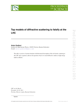
Figure 2.1: Constraints on ΛCDM model arising from CMB anisotropies, deep
galaxy samples, SNIa distribution and other data. This plot was drown in
2003; recent data are even more constraining.
As a matter of fact all available cosmological data can be fitted by ΛCDM
models. Figure 2.1 shows the constraints on such models, arising from CMB
anisotropies, deep galaxy samples and SNIa distribution, as they were around
2003. More recent data allowed to put much more stringent constraints and
confirm that the region of intersection is also associated to Ωb,o values which
agree with BBNS. The best–fit ΛCDM model, taking into account all the above
data, is also dubbed cosmic concordance model.
The old relativist idea that Λ is essentially a geometrical constant is not
an explanation, but just a way to rephrase the problem. The quest for the
physical origin of a cosmic component with widely negative pressure is then
open.
A firm point is that there is no ordinary free particle distribution which
allows for negative pressure. Let F (x, p, τ ) be the distribution of any set of free
particles in the phase space, yielding the distribution f (p, τ ) in the momentum
space in the homogenous case. The components of the stress energy tensor,
for such particle distribution, read
Z 3
dp µ
µ
Tν =
p pν f (p, τ )
(2.4)
p0
so that
ρ≡
T00
=
Z
3
0
d p p f (p, τ ) ,
3P ≡
Tii
16
=
Z
µ
m2
dp p − 0
p
3
0
¶
f (p, τ ) .
(2.5)
2.3. False vacuum ad Dark Energy
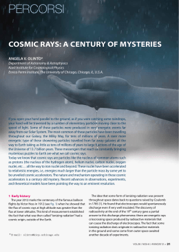
Figure 2.2: φ dependence of Coleman–Weinberg potential when T decreases
from T5 to T1 . For the sake of simplicity, potentials were plotted so to coincide at φ = 0. The 0–level of energy, however, varies with T and coincides
with the absolute minimum in each curve. Accordingly, for any T > T2 , the
configuration φ = 0 corresponds to the true vacuum. When T < T2 , instead,
the true vacuum corresponds to a configuration with φ 6= 0 (spontaneous symmetry breaking), while the symmetrical configuration φ = 0, which could be
temporarily stable, yields a false vacuum state. The vacuum energy density
ρv , in such state, is the difference between the levels of the local and global
minima; the vacuum pressure is then Pv = −ρv .
Eqs. (2.5) shows that ρ = 3P , for any particle distribution, as soon as m ≪ p0 ;
they also show that, in order that P < 0, it should be m > p0 , as is for
tachions.
Besides of ordinary free particles, however, we may consider a false vacuum.
This idea was introduced in the context of relativistic phase transitions. The
potential (density) for a Higgs field, e.g., could have a Coleman–Weinberg
behavior (see Figure 2.2), so allowing for a false vacuum component.
It is well known that relativistic phase transition occurred during the early
cosmic expansion. The last of such transitions has probably occurred at a temperature Tew ≃ 100 GeV, when the SUL (2) ⊗ UY (1) symmetry of electroweak
interaction has broken, so that the only remaining gauge symmetry is Uem (1)
and the only massless gauge field is the photon.
When the cosmic temperature was ∼ Tew and before the symmetry breaking
occurred, the Universe layed in a false vacuum state whose energy density was
17
2. The dark side of the Universe
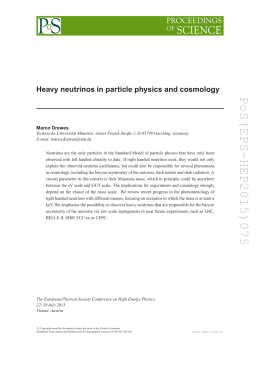
Figure 2.3: Evolution of energy density for DE, DM, radiation and baryons in
a ΛCDM model.
4
. When the passage to the true vacuum state finally occurred, this
ρv,ew ∼ Tew
coherent energy was thermalized.
4
with the energy density of a present false vacuum
It is easy to compare Tew
state, assumed to cause the cosmic acceleration. The present critical density
is ≃ 0.25 h−2 10−4 (π 2 /15)To4 ; here (π 2 /15)To4 is the energy density of CMB
radiation, whose temperature is To ≃ 2.3 eV. Accordingly, we should have
that Λ ∼ (10To )4 so that
Λ ∼ (10To /Tew )4 ρv,ew ≃ (10−2.5 /1011 )4 ρv,ew ≃ 10−52 ρv,ew .
(2.6)
This is still an optimistic view, as others believe that the fair comparison to
be made is with Planck energy density.
Besides of this fine tuning problem, ΛCDM models suffer of a severe coincidence problem, illustrated in Figure 2.3, making clear that vacuum energy
density became a significant cosmic component only quite recently. This fact,
by itself, appear a rather peculiar coincidence. But there is more: the linear growth of any cosmic inhomogeneity is severely suppressed when vacuum
energy density becomes significant and would be stopped if such component
is dominant. Therefore, e.g., if ρv were 10 times greater than observed, no
significant large scale structure could form in the Universe. It is as though ρv
had been wisely tuned, a priori, just to allow cosmic structures to arise.
18
2.4. Dynamical Dark Energy
2.4
Dynamical Dark Energy
In order to ease the above fine tuning, an alternative option is to have recourse
to a scalar field φ, self–interacting through an effective potential V (φ). Under
suitable conditions, such a component has widely negative pressure. Notice,
however, that this approach will not ease the coincidence problem. Moreover
we shall then make clear why this substance is to be treated as a field instead
of quanta.
From the φ field lagrangian we can then derive the stress–energy tensor of
the DE field and, from its components, we have
ρde = ρk + ρp ,
with
Pde = ρk − ρp
2
ρk = φ′ /2a2 , ρp = V (φ) ,
(2.7)
(2.8)
being the kinetic and potential energy densities of φ (in this section I shall
mostly use the conformal time τ and set ′ ≡ d/dτ ). Either from the Euler–
Lagrange equation, or from the Friedmann eq.
ρ′de + 3(a′ /a)(3Pde + ρde ) = 0,
we then easily obtain the equation
a′
φ′′ + 2 φ′ + a2 V,φ = 0
a
(2.9)
to be integrated to obtain the time evolution of φ and, thence, of ρk , ρp , ρde
and Pde . From these variables we then obtain the time dependence of
w=
Notice then that it is also
ρk − ρp
ρk + ρ p
(2.10)
2
1+w
φ′
=2
(2.11)
a2 V
1−w
so that the DE state parameter w approches -1 only when the kinetic energy
vanishes. It is also important to notice that w ≃ 1 (stiff matter) for ρk ≫ V
(in the sequel, the state parameter w without index will always refer to DE).
Unfortunately, however, in order to integrate eq. (2.9), the τ dependence of
the scale factor a must be known. This is to be worked out from the Friedmann
equation
µ ′ ¶2
a
8π
Gρa2
=
(2.12)
a
3
(we assume a vanishing spatial curvature K), which can only be integrated
once the τ dependence of ρ is known. Accordingly, either ρde ≪ ρ, as can be in
the early Universe, or eqs. (2.9) and (2.12) ought to be simultaneously solved,
as a system of equation, by using suitable numerical techniques.
19
2. The dark side of the Universe
Table 2.1: Some scalar field potentials usually studied in dark energy models.
Scalar field potential
V (φ) =
Λ4+α
φα
V (φ) =
2
Λ4+α κ
e2φ
φα
Reference
Ratra & Peebles 1998 [43]
κ = 8πG
Brax & Martin 2000 [51]
V (φ) = Λ4 e−λφ
Wetterich 1988, Ferreira & Joyce 1998 [45]
V (φ) = Λ4 [eακφ + eβκφ ]
Barreiro, Copeland & Nunes 2000 [46]
V (φ) = Λ4 [1 + cos φf ]
Kim 1999 [47]
V (φ) = Λ4 [(φ − B)α + A]e−λφ
Albrecht & Skordis 2000 [48]
V (φ) = Λ4 [cosh(λφ) − 1]p
Sahni & Wang 2000[49]
As a matter of fact, in early epochs, when the contribution of DE was
negligible or sub–dominant, the expansion rate depends almost exclusively on
the cosmic component whose density prevails.
Accordingly, H(τ ) ≡ a′ /a depends on the dominant component and this
changes the behavior of φ(τ ), according to eq. (2.9). Therefore, the equation
of state of DE depends on the cosmic component dominating the expansion in
each cosmological epoch.
Quite in general, the solution of a differential equation depends on the initial conditions. There exists however a class of potentials V (φ) which own an
attractor solution, i.e., such that – almost indipendently from the initial conditions set well inside the radiative epoch –, at any relevant epoch the behavior of
φ(τ ) does not depend on the assigned initial conditions. These potentials are
defined tracker potentials and the attractor solutions are denominated tracking
solutions.
Much work has been done to find out tracker potentials. In Table 2.4 we
list some of the tracker potentials.
This kind of DE, due to a scalar field dynamics is dubbed dynamical DE
(dDE) or quintessence.
Among these potentials I shall often select the SUGRA potential
V (φ) = (Λ4+α /φα ) exp(4πφ2 /m2p )
(2.13)
introduced by Brax & Martin [44] (see also [50, 51]). Here mp = G−1/2 is the
Planck mass. This potential has been shown to fit all available data at least
as well as ΛCDM (Colombo & Gervasi 2006).
20
2.5. Coupled Dark Energy
It can be verified that, starting from a tracking solution, this potential
yields that φ ∼ mp today, when V (φ) ∼ ρo,cr . Accordingly, we must have
Λ4 (Λ/mp )α ∼ (10 To )4
(2.14)
and, e.g. for α = 4, this yields
√
Λ ∼ 1028 × 10−2.5 eV ∼ 103 GeV
an energy range familiar to particle physics, where the electroweak transition
and/or the soft SUSY break may occur.
Accordingly, a dDE approach does not seem to require the introduction of
fine–tuned energy scales.
It has however been outlined that this result is made possible by the tiny
mass the φ field must have, in order that quintessence behaves as a field,
its quanta being essentially delocalized. According to some researchers, this
reintroduces a sort of fine tuning.
2.5
Coupled Dark Energy
The essential feature of the scalar field φ, in order that it yields DE, is its self–
interaction through a potential V (φ): when the self–interaction term dominates
energy density and pressure achieve opposite signs.
Altogether, therefore, in dDE theories, the φ field must interact with itself
and with the gravitational field.
It is then natural to wonder whether any other interaction is allowed to
it. If DE is coupled to another cosmic component, its stress–energy pseudo–
µ
conservation equation, Tν;µ
= 0 (µ, ν = 0, 3) would be modified. The simplest
form of possible coupling is a linear one. It can be formally obtained by
performing a conformal transformation of Brans–Dicke theory (see e.g. [52] ),
where gravity is modified by adding a φR term (R is the Ricci scalar) to the
Lagrangian.
Interactions with baryons are constrained by observational limits on violations of the equivalence principle (see, e.g., [53, 54]) No similar constraints hold
for DE–DM interactions. In this case, constraints will follow from cosmological
observations.
The option of DE–DM coupling was considered several times in the literature, starting from Wetterich (1988) [55]. Its physical effects were then
discussed more in detail by Amendola (1999, 2000) [52, 56] and Holden &
Wands (2000) [57], who stressed that, owing to the vanishing of the trace of
Tµν for zero–mass components, no photon and neutrino interaction with DE follows. Theoretical motivations for DE–DM coupling were found, in superstring
models and in brane cosmology, by Gasperini, Piazza & Veneziano (2002) [58].
(φ)
(c)
Let then Tµν and Tµν be the stress–energy tensors of a scalar field φ and
DM, respectively. Leaving apart the connection with Brans–Dickie cosmology,
21
2. The dark side of the Universe
we may then notice that general covariance itself requires that the total stress–
energy tensor Tµν fulfills the continuity equation
T µν;µ = 0 ,
(2.15)
but it does not prevent an interaction between DE (the φ field) and DM such
that
µ
T (φ) ν;µ = +CT (c) φ;ν ,
µ
T (c) ν;µ = −CT (c) φ;ν .
(2.16)
As is known, eq. (2.15) tells us how the 4–momentum components evolve under
the action of gravity. In the absence of gravity, they yield the conservation of
momentum and energy. Accordingly, the coupling described by eqs. (2.16)
accounts for a transfer of energy and momentum between DE and DM.
The analytical treatment of a coupled DE model (cDE) is clearly more
involved than dDE, in particular for what concerns the dynamics of density
fluctuations. Thy are usually treated either in the synchronous or in the Newtonian conformal gauge. Assuming zero spatial curvature, in the former case
we the FRW metric becomes
ds2 = a2 (dτ 2 − ηij dxi dxj ) .
(2.17)
If xα (α = 1, 2, 3) are cartesian orthogonal coordinates, it is ηij = δij + hij , so
that any peculiar gravity due to density fluctuations is described by hij . In
the latter case, instead,
ds2 = a2 (τ )[(1 + 2Φ)dτ 2 − (1 − 2Ψ)dxi dxi ]
(2.18)
and, in the absence of anisotropic stresses, peculiar gravity is fully described
by the potential Ψ = Φ.
In the former case, the conformal time τ is universal, in the latter case it
depends on the site.
In the absence of fluctuations, in the frame of reference where the metric
is FRW, eqs. (2.16) yield:
φ′′ + 2Hφ′ + a2 V,φ = Cρc a2 ,
ρ′ c + 3Hρc = −Cρc φ′
(2.19)
(2.20)
An analysis of background expansion in the presence of coupling has been
performed by various authors [55, 59, 52, 56, 57, 58]. The equations yielding
the behavior of the different cosmic components are formally simpler if the
following five variables are used:
r
r
r
κ φ′
κ V
κ ργ
κ ρb
x= √ , y=
, z=
, v=
,
(2.21)
H 6
H 3
H
3
H 3
22
2.5. Coupled Dark Energy
ργ and ρb being the energy densities of radiation (including neutrinos, assumed
to be massless) and baryons, respectively. Here κ2 = 8πG; furthermore, H =
Ha is the usual Hubble parameter.
x2 , y 2 , z 2 and v 2 coincide with : the density parameter of the kinetic
component of φ and the potential components of φ, radiation and baryons,
respectively. The cold DM energy density parameter is obviously Ωc = 1 −
x2 − y 2 − z 2 − v 2 .
The potential V (φ) defines a function f (φ) through to the relation
√2
(2.22)
V (φ) = Ae−κ 3 µf (φ)φ ,
which also depends on the choice of the dimensionless constant µ. The exponential case (Wetterich 1995, Amendola 2000) corresponds therefore to f = 1,
a constant potential [60] to µ = 0, the power law V ∼ φ−α to f (φ) =
p
κ
−α 2φ2
to f (φ) =
p(3/2)α log φ/(κµφ), and a SUGRA type potential V ∼ φ e
(3/2)[α log φ/(κφ) − κφ/2]/µ.
It is then also convenient to take as independent variable la ≡ log a, instead
of the scale factor a or the time t.
If differentiation in respect to la is still indicated by a prime, the Einstein equations and the conservation equations, for the components of the
4–momentum of the scalar field, radiation, baryons and CDM then read
¶
µ ′
z
′
− 1 x − µf1 y 2 + β(1 − x2 − y 2 − v 2 − z 2 ),
x =
z
µ
¶
z′
′
y = µf1 xy + y 2 +
,
z
¢
z¡ 2
3x − 3y 2 + z 2 − 1 ,
z′ =
2
¢
v¡ 2
′
(2.23)
3x − 3y 2 + z 2 .
v =
2
Here
β=
p
3/2κ2 C = (3/π)1/2 (C/mp )
(2.24)
is a dimensionless parameter suitably gauging the interaction strength, while
df
+f .
f1 = dφ
Note that the system (2.23) is subject to the condition x2 +y 2 +v 2 +z 2 ≤ −1.
To close the system one needs also the Friedman equation
¢
1¡
H′
= − 3 + 3x2 − 3y 2 + z 2 .
H
2
(2.25)
On the basis of these equations the time dependence of the density parameters
is obtainable.
Some early work on cDE apparently allowed to ease the coincidence problem. Some evidence of how this occurred is still exhibited in the Figure.
23
2. The dark side of the Universe
In fact, starting from a tracker solution, at recombination, DE energy density is mostly due to its kinetic component and, therefore, wde ≃ 1. Because
of the coupling, energy is transferred from DM to DE, where it dilutes ∝ a6
and is so washed away. This however allows ρde to keep to a significant level
which, for large β values, can be comparable with DM. In turn, because of the
coupling, ρc also declines in time more rapidly than a3 . This kind of evolution
approaches an end when φ becomes so large that V (φ) is no longer negligible.
Then ρde rapidly increases and overcomes ρc .
For β ∼ O(1), DM and DE exhibit then an almost parallel behavior, since
recombination to the eve of the present epoch. DE, therefore, is a significant
portion of the Universe contents at z ∼ 103 , so easing the coincidence problem.
A careful comparison with observational data, however, led to exclude β
values above ∼ 0.07–0.1, at the 3–σ level. Accordingly, cDE could hardly be
“used” to ease coincidence.
In chapter 3, however, we show greater couplings, made compatible with
data by the symultanous presence of significant ν masses.
The maximum β considered in the Figure, however, is still 0.21. By using
a Fisher matrix technique, it appears to be consistent with available data at
the 2–σ level, so pushing upward observational limits on β by more than a
factor 2.
It must be acknowledged that the easing of the coincidence problem, even
with β ∼ O(0.2), is not completely satisfactory. However, once the gene has
escaped from the bottle, it is almost impossible to put him back inside and
cDE models need to be confirmed or excluded by data.
2.6
Fluctuation dynamics and its Newtonian
limit
If fluctuations are then considered, in respect to the FRW background, besides of metric fluctuations we shall have density fluctuations in the various
components as well as in the DE field φ.
Let then be δ = δρ/ρ for DM, baryons and radiative components. Radiative
components will be however scarcely relevant here. Let vi be the velocity field
components for each cosmic component, and let be θ = ∇i vi . For both δ and
θ, I shall use an index c or b , to indicate DM or baryons.
A Fourier expansion of density perturbation shall be performed, in order
to separate te behavior of different k–harmonics. In the equations, the wave
number k will appear through the adimensional variable
λ = H/k.
(2.26)
Besides of the background component, that I shall now indicate φo , the
scalar field will also have a perturbation, so that φ = φo + δφ. It is then
24
2.6. Fluctuation dynamics and its Newtonian limit
convenient to define the adimensional field perturbation variable
√
ϕ = κ δφ/ 6 .
(2.27)
I shall also use the adimensional mass of the scalar field, defined according to
mφ = Vφ′′ a/H
(2.28)
Using these variables, the equations for the different components, in the conformal newtonian gauge, read:
DM
δc′ = −θc + 3ψ ′ − 2βϕ′ − 2β ′ ϕ ,
¶
µ
H′
′
− 2βx θc + λ−2 (ψ − 2βϕ) ,
θc = − 1 +
H
(2.29)
(2.30)
Baryons
δb′ = −θb + 3ψ ′ ,
µ
¶
H′
− 2βb x θb + c2s λ−2 δ + λ−2 ψ,
θb′ = − 1 +
H
(2.31)
(2.32)
Scalar field
¡
H′ ¢ ′
ϕ
ϕ′′ + 2 +
ϕ + (λ−2 + m̂2φ )ϕ − 4ψ ′ x − 2y 2 µf1 ψ = βΩc (δc + 2ψ) + Ωc β ′ ,
H
x
Metric
P
−3λ2 [6xϕ + 2xϕ′ − 2y 2 µf1 ϕ + Ωi (δi + 3(wi + 1)λ2 θi )]
, (2.33)
ψ =
2(1 − 3λ2 (x2 + 2y 2 ))
X
1
ψ ′ = [2(3xϕ − ψ) + λ2
(2.34)
3(wi + 1)θi Ωi ].
2
We omit here the equations for radiation and (massive) neutrinos. Their treatment has however just the standard complications. When the Universe gradually recombines, more and more spherical harmonics of photon and ν distributions ought to be considered. In the case of massive ν, whose distribution
evolution, in the configuration space, depends on momentum, also the latter
variable is to be suitably sampled.
Quite in general, however, such a system of differential equations requires
a numerical solution. We obtained them suitably modifying public programs,
like CMBFAST and CAMB, as well as through our own program, yielding high
precision results.
It is also important to consider it in the Newtonian limit, as it was used to
perform n–body simulations (Macció et al 2005).
Taking a Newtonian limit means going to small scales, λ << 1. Keeping
just the lowest order terms in λ, the gravitational and ϕ field equations then
read
3
ψ = − λ2 (Ωb δb + Ωc δc + 6xϕ + 2xϕ′ − 2y 2 f1 ϕ) , ψ ′ = 3xϕ − ψ ,
(2.35)
2
25
2. The dark side of the Universe
′
¡
H¢ ′
ϕ + λ−2 ϕ − 12xϕ + 4ψx + 2y 2 (f2 ϕ − f1 ψ) = βΩc (δc + 2ψ). (2.36)
ϕ′′ + 2 +
H
df
Here f2 = φ dφ
+ 2f + f1 . If DE kinetic (and/or potential) energy substantially
contributes to the expansion source, x (and/or y) is O(1).
In the Newtonian limit, we must also neglect the derivatives of ϕ, averaging out the oscillations of ϕ and the potential term f2 y 2 ϕ, requiring that
λ << (f2 y)−1 (remind that y is O(1)). Furthermore, in eq. (2.36), the metric
potential ψ (∝ λ2 ) can also be neglected. Accordingly, eq. (2.35) and (2.36)
become
3
(2.37)
ψ = − λ2 (Ωb δb + Ωc δc ), , λ−2 ϕ ≃ βΩc δc .
2
(the former one is the usual Poisson equation). If we substitute in (2.30) we
can define a new potential acting on DM
3
3
4
ψc = ψ − 2βc ϕ = − λ2 Ωb δb − λ2 Ωc δc (1 + β 2 ) .
2
2
3
(2.38)
In real space, this equation becomes
∇2 Φc = 4πGρb δb + 4πG∗ ρc δc ,
(2.39)
so that G∗ = γG with γ = 1+4β 2 /3. For the velocity fields θc,b we then obtain:
¢ 3¡
¡
3
H′
4 ¢
θc ′ = −θc 1 +
− 2βx − 1 + β 2 Ωc δc − Ωb δb , ,
H
2
3
2
¡
H′ ¢ 3
θb ′ = −θb 1 +
− (Ωc δc + Ωb δb ) .
H
2
(2.40)
(2.41)
Deriving eqs. (1.28) and (1.30) and taking the Newtonian limit (λ << 1) one
can obtain a couple of equations telling us how δc,b and θc,b depend on a:
¢ 3
¡
4
3
H′
− 2βx + (1 + β 2 )Ωc δc + Ωb δb ,
δc ′′ = −δc ′ 1 +
H
2
3
2
′¢
¡
3
H
δb ′′ = −δb ′ 1 +
+ (Ωc δc + Ωb δb ),
H
2
(2.42)
(2.43)
R
Assuming Ωb << Ωc and putting δc ∝ e η(α)dα and δb = bδc with b = cost
from the eqs.(2.42), (2.43), we obtain the bias factor
b=
δb
3Ωc
.
≃
δc
3γ Ωc + 4β xη
(2.44)
The acceleration of a single DM or baryon particle of mass mc,b can be instead
derived from eqs. (2.40), (2.41). Let us set it in the void, at a distance r from
the origin, where a DM (or baryon) particle of mass Mc (or Mb ) is set, and let
us remind that, while the usual scaling ρb ∝ a−3 holds, it is
ρc = ρoc a−3 e−
R
C(φ)dφ
, ρMc = Moc a−3 e−
26
R
C(φ)dφ
δ(0),
(2.45)
2.6. Fluctuation dynamics and its Newtonian limit
because of the DE-DM coupling (here the subscript o indicates values at the
We can then assign to each DM particle a
present time τo (it is ao = 1)).
R
varying mass Mc (φ) = Moc e− C(φ)dφ
Then, owing to eq. (2.45), and assuming that the density of the particle
widely exceeds the background density, it is
ρ Mc − ρ c
8πG
ρ Mb − ρ b
8πG
Mc (φ)δ(0) , Ωb δb =
Mb δ(0),
=
=
ρcr
3H2 a
ρcr
3H2 a
(2.46)
(ρcr is the critical density and δ is the Dirac distribution). Reminding that
∇ · vc,b = θc,b H and using the ordinary (not conformal) time, eq. (2.42) yields
Ωc δc =
∇ · v̇c = −H(1 − 2βx) ∇ · vc − 4πGa−2 (γMc (φ) + Mb ) δ(0)
(2.47)
(dots yield differentiation in respect to ordinary time and H = ȧ/a). Taking
into account that the acceleration is radial, as the attracting particles lie at
the origin, it will be
Z
Z
d3 r ∇ · v̇ = 4π dr d(r2 v̇)/dr = 4πr2 v̇.
Accordingly, the radial acceleration of a DM particle read
v̇c = −(1 − 2βx)Hvc · n −
G∗ Mc (φ) GMb
−
,
R2
R2
(2.48)
(n is a unit vector in the radial direction; R = ar). Repeating the calculation
for a baryon we get immediately the result
v̇b = −Hvb · n −
GMc (φ) GMb
−
R2
R2
(2.49)
In eq. (2.48) the three effects of the coupling appear clearly: the masses
of DM particles depend on the time evolution of φ; their variation induces an
extra friction −2βx in the equation of motion (2.48); a different gravity is felt
by DM with respect to baryons.
The dimensionless constant β 2 yields the ratio between the DM–DM gravitational constant and usual gravity:
¶
µ
4β 2
∗
.
(2.50)
G =G 1+
3
In fact baryons, which remain uncoupled (or very weakly coupled) to DE,
keep the usual gravitational behavior. G∗ holds just for interactions between
DM particles, whose motions violate the equivalence principle, although this
is unobservable with local experiments.
27
Chapter
3
Softening limits on neutrino
mass through DM–DE coupling
Cosmological limits on neutrino masses are softened, by more than a factor 2, if
Dark Matter and Dark Energy are coupled. In turn, a neutrino mass yielding
Ων up to ∼ 0.20 allows coupling levels β ≃ 0.15 or more, already slightly
easing the coincidence problem. The coupling, in fact, displaces both P (k)
and Cl spectra in a fashion opposite to neutrino mass. Tentative estimates are
obtained through a Fisher–matrix technique and typical examples are obtained
by exploring the parameter space.
The results described here are refered in part to a paper published by the
author [61].
3.1
Introduction
There seem to be little doubt left: at least one neutrino mass eigenstate or,
possibly, two of them exceed ≃ 0.055 eV (direct or inverse hierarchy). This
follows solar [62] and reactor [63] neutrino experiments, yielding ∆m21,2 ≃ 8 ×
10−5 eV2 and, namely, atmospheric [64] and accelerator beam [65] experiments
yielding ∆m22,3 ≃ 3 × 10−3 eV2 .
Cosmology is also sensitive to neutrino mass. Valdarnini & Bonometto
(1984) [66] made a detailed analysis of transfer functions in cosmologies where
a part of Dark Matter (DM) is due to massive neutrinos, so proposing mixed
DM models, where neutrinos play an essential role in adjusting CMB (Cosmic Microwave Background) anisotropies and matter fluctuation spectra to fit
observations. A large deal of work on this subject took place in the Nineties;
mixed models were widely tested, using both the linear and the non–linear
theory.
Hubble diagram of SNIa [67] showed then an accelerated cosmic expansion,
while advanced data on CMB [68] and large scale structure [69] required a
spatially flat cosmology with a matter density parameter Ωo,m ≃ 0.27, so that
29
3. Softening limits on neutrino mass through DM–DE coupling
the gap up to unity was to be filled by a smooth non–particle component
dubbed Dark Energy (DE).
All that relegated neutrinos to a secondary role in shaping cosmic data
while, by using such advanced astrophysical data, increasingly stringent limits
on neutrino masses could be computed (see, e.g. [70])
Standard limits on neutrino masses were recently summarized by Komatsu
et al (2008) [71], within the WMAP5 release, and are quoted in Table 3.1.
More stringent but more speculative limits are suggested in [72], who make a
more extensive use of SDSS or 2dF data, and in [73], by using Lyα forest data.
These limits, clearly, rely on implicit assumptions concerning the dark cosmic sector, whose knowledge still fully relies on astrophysical data, requiring
two components characterized by state parameters w ≃ 0 and ≃ −1. But the
assumption that no energy exchange between them occurs, tested vs. data,
leads just to coupling limits.
As we showed in Chapter 2, a large deal of work dealt with the coupling
option, in the attempt to overcome the coincidence paradox. All that makes
our epoch unique and, unless one indulges to anthropic views, apparently requires an explanation. However, also indipendently from this conceptual issue,
our very ignorance of the physics of the dark sector requires that all reasonable
options consistent with basic physics and data are explored.
It is also important to outline that neutrino mass limits can be softened
if DE with a state parameter w < −1 is considered [74]. Unfortunately, this
kind of state equations, yielding the so–called phantom–DE, can be justified
only making recourse to unconventional physics.
In this section we show that spectral distortions due to DM–DE coupling
and to neutrino mass tend to compensate. We tentatively estimate how far we
can go, simultaneously increasing coupling and mass, by using a Fisher Matrix
(FM) technique. On that basis we perform a preliminary exploration of the
parameter space, substantially confirming FM findings.
3.2
Some angular and linear spectra
The point of this paper can be appreciated through the spectra in Figures
3.1 and 3.2. We compare a model with zero coupling and zero neutrino mass
(00–model, hereafter) with: (i) a model with 2 massive neutrinos with mass
mν = 0.119 eV, yielding Ων = 0.005 (plus 1 massless neutrino); (ii) a model
with a DM–DE coupling β = 0.049; (iii) a model with both neutrino mass and
Table 3.1: Summary of the 2–σ (95% C.L.) constraints on the sum of ν masses,
from WMAP 5-year and other cosmological data sets.
w = −1
< 1.3 eV
< 0.67 eV
WMAP5
WMAP5+BAO+SN
30
w 6= −1
< 1.5 eV
< 0.80 eV
3.2. Some angular and linear spectra
0.1
1
Figure 3.1: Transfer functions in cosmologies with/without coupling and
with/without 2 massive neutrinos. Coupling and mass are selected so to yield
an approximate balance. The functions are multiplied by k 1.5 , to help the
reader to distinguish different cases.
coupling (CM–model, herafter). All models are spatially flat, have adimensional Hubble parameter h = 0.71, density parameters Ωb = 0.04, Ωde = 0.73,
spectral index ns = 0.96 and a cosmic opacity τopt = 0.089. DE is due to a
SUGRA potential with Λ = 1.1 GeV, fitting WMAP and other data at least
as well as a ΛCDM.
Angular and spatial spectra are computed with an extension of the program
CAMB, allowing to treat coupled DE models also in the presence of massive
neutrinos.
Both l and k ranges are selected for being those physically most significant.
At lower l’s model discrepancies essentially vanish. In the l region shown, we
have the sequel of maxima and minima due to primeval compression waves.
The k range covers the scale explored by deep samples, as 2dF or the SLOAN
digital survey, up to k values where non–linear effects become important.
In the plots, spectra are multiplied by suitable powers of the abscissa l or
k, so to reduce the ordinate range. In spite of that, in the Cl plot different
spectra are not easy to distinguish. We then plot also the ratio ∆Cl /Cl at
constant l; shifts would however appear even smaller if slight shifts along the
l axis (by 1 or 2 units) were performed.
The Figures are principally meant to show that the effects of neutrino
31
3. Softening limits on neutrino mass through DM–DE coupling
Figure 3.2: Angular anisotropy spectra for the same models of the previous
figure. Due to intrinsic Cl oscillations, this Figure is slightly harder to read.
In the lower frame we also give the spectral differences between 00– and CM–
models. Large l oscillations could be further damped by a shift by 1 or 2 units
along l. The dotted lines represent the cosmic variance interval.
mass and coupling are opposite. The coupling intensity, in fact, is selected so
to (approximately) balance neutrino masses.
P
We took, however,
mν ≪ 0.61 and β ≪ 0.075 (see Amendola 1999,
Amendola & Quercellini 2000, Macciò et al 2004); each of these values, by itself,
is within current observational limits. Accordingly, even the difference between
thin and thick solid–line spectra cannot be appreciated through current data.
In particular, let us outline how the BAO (baryonic acoustic oscillation)
structure is faithfully reproduced when passing from the 00–models (thick solid
line) to the CM–models (thick dashed line).
32
3.3. Fisher matrix
3.3
Fisher matrix
We then aim to test how far we can go, simultaneously increasing β and Ων ,
without conflicting with data. This can be estimated by using a FM analysis
[75, 76, 77] (see App. A.1).
This approach allows a rapid, semi–analytic estimate of the confidence limits for a specific experiment. It assumes a reference model as the most probable
~ of the data sysone, i.e. as the maximum of the likelihood distribution L(~x|θ)
tem ~x given the model, described by parameters θ~ ≡ (θi ). Exploiting this
hypothesis, one can approximate L by a multivariate Gaussian distribution,
built using its second derivatives in respect to the parameters (θ̄i ) at the reference model. Nevertheless, as is known, this technique is limited by the actual
non–Gaussian behavior of data.
3.3.1
Data and technique
In the literature, cosmological models are constrained by using a large number of observables. To our present aims we shall directly consider the spectrum of matter fluctuations P (k) and the CMB angular spectra ClXY (XY =
T T, T E, EE). In their recent analysis, Komatsu et al (2008) made a more restricted use of P (k), using only BAO’s, while they used SNIa Hubble diagrams,
so significant also for being the first signal of DE.
Here we chose observables directly coming from the model, in the attempt
to leave apart observational biases, focusing just on the level of sensitivity of
possible experiments. We consider then two different experimental contexts.
The first one assumes that CMB spectra are measured at WMAP sensitivity
and P (k) is measured with the sensitivity of the 2dF experiment (case W).
The second assumes Planck sensitivity for CMB spectra and SDSS sensitivity
for P (k) (case P). The observational features for each mission considered are
listed in Table 3.2 for the case of CMB experiments and in Table 3.3 for the
galaxy surveys.
Table 3.2: WMAP and PLANCK mission specifications used in the paper.
Mission
WMAP
PLANCK
lmax
1000
2500
fsky
0.8
0.8
θF W HM
13’
7.1’
σT
260
42
σP
500
80
Table 3.3: 2dF and SDSS–like mission specifications used in the paper. Scales
and volumes are in Mpc/h and (Mpc/h)3 , respectively.
Mission
2dF
SDSS
kmin
0.02
0.02
kmax
0.1
0.15
33
Volume
108
0.72×109
3. Softening limits on neutrino mass through DM–DE coupling
Let us now consider first the use of CMB data only and let ClXY be the
angular spectra of the input model, to which we must add a white noise signal,
to obtain
·
¸
θF2 W HM
XY
XY
XY
XY
2
with
Nl = δXY σX exp l(l + 1)
. (3.1)
C̄l = Cl + Nl
8 ln 2
The expressions of the Fisher matrix FCij components are then obtainable according to the relation
X X ∂
′ ′
XY X ′ Y ′ ∂
FCij =
ClXY [Cov−1
ClX Y
(3.2)
C ]l
∂θi
∂θj
l XY,X ′ Y ′
with

ClT E C̄lT T
.
ClT E C̄lEE
[CovC ]l
1
TE 2
T T EE
[(Cl ) + C̄l C̄l ]
2
(3.3)
On the contrary, when dealing with matter power spectra, we used the
following definition for the FM [78]
X ∂
∂
P (kα )[Cov−1
P (kβ )
(3.4)
FPij =
P ]αβ
∂θi
∂θj
α,β
XY,X ′ Y ′

(C̄lT T )2
(ClT E )2
1
TE 2

(Cl )
(ClEE )2
=
(l + 1/2)fsky
TE TT
Cl C̄l
ClT E C̄lEE
with
Vf
2P 2 (kα ) ,
(3.5)
Vs (kα )
where Vf = (2π)3 /V is the volume of the foundamental cell in k space, V is
the volume of the survey and Vs (kα ) = 4πkα2 δk is the volume of the shell of
width δk centered on kα [79, 80]. In eq.(3.5) we left aside the contribution of
the trispectrum, because in our analysis we considered only the linear scales,
where the trispectrum is negligible.
The cosmological model we consider is characterized by 9 parameters: ωb =
Ωb h2 , ωc = Ωc h2 density parameters for baryons and CDM, respctively, H0
Hubble parameter, As scalar fluctuation amplitude, ns spectral index, τopt
cosmic opacity to CMB photons, Log(Λ)/GeV logarithm
P of the energy scale in
SUGRA potential, β DM–DE coupling parameter,
mν /eV sum of neutrino
masses. We estimate the neutrino mass density parameter, Ων h2 , converting
it from the total neutrino mass via
P
mν
2
Ων h =
.
(3.6)
93.5 eV
We compute the CMB anisotropies (temperature and polarisation) power
spectra and the transfer functions, used to calculate linear matter power spectrum, using a modified version of the public available code CAMB1 . Numerical
derivatives were evaluated considering a 5% stepsize, except for Λ, where we
adopted a 5% stepsize on λ ≡ Log(Λ/GeV).
[CovP ]αβ ≃ δαβ
1
http://www.camb.info/
34
3.3. Fisher matrix
Figure 3.3: 1– and 2–σ confidence levels for a 2–massive–neutrino model, assuming that the true cosmology is a SUGRA model with log(Λ/GeV) = 1.1,
while β = 0 and Ων ≃ 0. Thick (thin) curves show the constraints deriving from
CMB and deep sample data (from CMB data only). Solid curves refer to the (i)
case (WMAP+2dF). Dashed curves refer to the (ii) case (PLANCK+SDSS).
In the sequel we shall examine in detail models corresponding to the points
labeled a, b, c, d, e and others. The location of the CM–model of Figs. 3.1 and
3.2 is indicated by an open box. The two locations indicated by an open circle
and a cross will also be considered in detail below. This Figure is somehow
analogous to Fig. 2 in Hannestad, 2005.
3.3.2
Results
In Figure
3.3 we then report the expected 1– and 2–σ likelihood curves on
P
the
mν –β plane, for both cases W and P. In either case we analyse the
constraints coming just from CMB data and those arising from the joint exploitation of CMB and deep sample data. We performed the analysis either
assuming 3 equal mass neutrinos, or 1 massless and 2 massive neutrinos. The
plots shown in the Figure are obtained for the latter case, but discrepancies
are just a minor effect.
35
3. Softening limits on neutrino mass through DM–DE coupling
0.25
0.2
0.15
0.1
0.05
0
0.02
0.021
0.1
0.12
70
75
80
0.25
0.2
0.15
0.1
0.05
0
-8.66
-8.64
-8.62 0.94 0.96 0.98
-1
0
1
0.06
0.09
0.12
Figure 3.4: Correlation between β and the other model parameters for the W
case (WMAP+2dF); dashed lines refer to CMB data only.
0.1
0.05
0
0.02
0.0204
0.105 0.112 0.119
70
75
80
0.1
0.05
0
-8.646 -8.64 -8.634
0.952 0.959 0.966
-0.3
0
0.3
0.08
0.09
0.1
Figure 3.5: Correlation between β and the other model parameters for the P
case (PLANCK+SDSS); dashed lines refer to CMB data only.
The Fisher–matrix results, for the W case, substantially confirms known
1– and 2–σ limits onP
β, yielding β < 0.05 and β < 0.075, respectively, along
the β axis (i.e. with
mν = 0).
P
On the other axis, with β = 0, Pmν seems to be P
more constrained than
mν < 0.8 with w 6=
what we know from current limits (
mν < 0.35 vs.
−1). These discrepancies can be read as an indication of the level or reliability
that Fisher–matrix estimate can have. In particuilar, they may be partially
due to the impact of using the whole P (k) information, as well as to the fact
that the reference cosmology is SUGRA instead of ΛCDM. However, the CMB
36
3.3. Fisher matrix
Figure 3.6: 1– and 2–σ limits, for the P–case, assuming that the true cosmology
corresponds to the points marked by cross or open circle. The dashed lines
report the same limits around the 00–model, as shown in Fig. 3.3; similarly,
the dotted line is the 1–σ limit around the 00–model in the W–case, as shown
in Fig. 3.3. This Figure shows that cosmologies, comprising DM–DE coupling
and neutrino masses, presently compatible with the 00 option, will be easily
discriminated, at the P sensitivity level.
P
2–σ
constraint
we
find,
mν < 1.65 , is close to the 95 % confidence limit
P
mν < 1.5 obtained through a full MonteCarlo analysis of WMAP data only,
with w 6= −1.
The likelihood plots have theP
expected shape. Taken at face value they
yield upper limits β . 0.22 and
mν . 1.05 eV , in the case W. With the
value of Ho used here this would correspond to Ων ≃ 0.022, almost 2/3 of
baryon density.
On the contrary, in theP
case P, constraints are more severe, as only CM–
models with β < 0.07 and
mν < 0.4 appear consistent with the 00–model,
at the 2–σ level. These limits are close to the maximum coupling and neutrino
mass separately admitted in the present observational constraints.
In Figure 3.4 we also show the correlations between β and the whole set of
37
3. Softening limits on neutrino mass through DM–DE coupling
parameters considered, in the W case. Correlations can be considered negligible for the parameters As , ns , Λ, τopt . The correlations with the parameters
ωc , ωb , Ho , as expected, are stronger.
Figure 3.5 yields analogous results for the P case. The same comments here
above hold for this case, just within the more constrained intervals allowed.
It may also be useful to consider Figure 3.6, showing that models, including
DM–DE coupling and neutrino masses, compatible with the 00 option at the
W sensitivity level, at the P sensitivity level will be well discriminated from it
and between them.
3.4
Exploring the parameter space
A further insight into FM results can be gained by considering a few examples.
In Figures 3.7 and 3.8 we exhibit the spectra for a set of models. As shown in
the frame of Fig. 3.7, the models yielding the maximum DM–DE coupling (and
vanishing ν mass) or the maximum neutrino mass (and vanishing coupling)
have the thick line spectra. Model discrepancy is enhanced by taking the same
amplitude As , instead of normalizing them to the
P same σ8 .
The setting of models a, b, c, d, e on the
mν –β plane is indicated in
Fig. 3.3. They are all on the 1–σ boundaries. The best performance, perhaps,
can be ascribed to models d and e. Both of them yield a present hot dark
matter density exceeding 1 % of the critical density and 5 % of the whole DM.
3.5
Conclusions
In this section we performed a first inspection on the possibility that high ν
masses and DM–DE coupling yield compensating distortions of matter fluctuations and CMB spectra. This compensation is highly effective for small
masses and couplings, as shown in Figs. 3.1 and 3.2. We then address the
most significant question concerning the limits on coupling and ν masses, when
simultanously considered.
This question should be carefully addressed by using MonteCarlo techniques and considering all available observational constraints. Unfortunately,
to do so, we should widen the usual parameter space, by adding 3 extra degrees of freedom: the coupling parameter β, neutrino mass, and the energy
scale Λ in the SUGRA model (or another equivalent parameter, in the same
or in another dynamical DE potential).
This is among the reasons that led previous authors to perform a preliminary test by using a Fisher matrix technique. Here we implemented such test
by exploring the parameter space under the guide of Fisher matrix outputs.
We reserve the MCMC analysis for a future work.
Taking Fisher matrix outputs at face value leads to state that models with
Ων . 0.022 and β . 0.22 are observationally consistent with a Ων = 0 and
38
3.5. Conclusions
Figure 3.7: Spectra for a number of cosmologies. All of them are obtained
setting ns = 0.96 and log As = −8.64, so to enhance model differences. Thick
lines correspond to models presentlyP
considered in agreement with data, and
yielding maximum values either for
mν or β. The other lines yield models
corresponding to the points a, b, c, d, e in Fig. 3.3, consistent with the 00–
model at the 1–σ level.
β = 0 model. We then directly explored the parameter space and confirmed
that a model with Ων ≃ 0.015 and β ≃ 0.1 appears in fair agreement with the
observables considered. Direct inspection on Ων ∼ 0.022–β ∼ 0.22 is not so
satisfactory.
This just confirms the expected limits of the Fisher matrix technique, but
we do expect similar values to be in agreement with the present observations
if the whole parameter set is suitably tuned. This “extreme” regime will be
easily falsified by experiments with a sensitivity comparable with PLANCK
and SDSS, as Figure 3.6 shows.
In turn, such experiments could lead to a safe detection of neutrino masses
widely exceeding microphysical data from flavor mixing. A mass range yielding
Ων ∼ 0.02 would mean that hot DM is ∼ 10 % of the DM total, so that its
effects significantly contribute to shaping large scale structure, as in old mixed
39
3. Softening limits on neutrino mass through DM–DE coupling
WMAP5
WMAP3
Figure 3.8: Spectra of CMB anisotropies for the same cosmologies of Fig. 3.7,
compared with WMAP error amplitudes. Let us remind that all of them are
obtained keeping the same values ns = 0.96 and log As = −8.64, so to enhance
model differences. The relative difference of the thick line models from the
00–model appears not so wide as for some of the other models. Among them,
however, the solid and dashed line models seem to perform quite well. Their
performance can be improved by adjusting the Ho value, slightly modifying
Fisher matrix outputs.
matter models.
Such “extreme” models would also achieve another important result. Models with cDE were initially considered to overcome the coincidence problem, in
the presence of DE. In Figure 3.9, we show theP
scale dependence of the density
parameters, for various models with different
mν and β.
In the usual case, with negligible mν , a DM–DE coupling compatible with
data hardly eases the coincidence problem. Such easing is represented by the
plateau in the Ωde curve, whose proportions are then almost unsignificant. This
does not mean that β 6= 0 is not to be considered among the possible degrees
40
3.5. Conclusions
Figure 3.9: Density parameters for cold DM, hot DM (ν’s), DE and radiation
in models with Ων and β taking the values 0.005–0.049 (short dashed), 0–0.07
(long dashed), 0.011–0.1 (dotted), 0.02–0.21 (solid), respectively. In the last
case, the DE plateau, extending up to the equatlity redshift, uccurring slightly
above z ∼ 103 , shows a DE density keeping ∼ 1/20 of cold DM.
of freedom; e.g., Vergani et al. (2008) have shown that a cosmology with β
as small as ∼ 0.05, if inspected assuming β ≡ 0, can yield badly wrong values
for some cosmic parameters, including ωoc . Figure 3.9 however indicates that,
when β ∼ 0.02 is recovered, in the presence of suitably massive ν’s, a significant
plateau is present and DE density keeps at the level ∼ 1–2 % of the critical
density up to z ∼ 103 .
41
Chapter
4
Weak Lensing properties
Weak gravitational lensing directly probes matter distribution, through its
gravitational potential, and, in principle, does so in any celestial site, requiring
no peculiar distribution of cosmic objects. Matter distribution, then, is much
more directly related to theoretical predictions than light distribution. In this
chapter I develop some of the formalism used to reconnect this phenomenon
to theory.
4.1
Basics of gravitational lensing
Light rays are deflected by any gravitational field. Deflection becomes observable if produced by quite a massive body. The possibility of light deflection
had been suspected since 1704, by Newton in the first edition of his Opticks.
This idea was subsequently pursued, in the context of a corpuscular theory of
light using Newton’s law of gravitation, by Cavendish (1784), Laplace (1796),
and Soldner (1801). After Maxwell electro–magnetic unification, light wave
deflection could also be confirmed. Nevertheless, General Relativity (GR) put
lensing on a firm theoretical footing, and yields twice the Newtonian value for
the deflection angle [81]. The agreement of this prediction with the deflection
of light from distant stars by the Sun, claimed for the solar eclipse of 1919
[82], was considered a great success for Einstein’s theory and brought General
Relativity to the general attention. More recent experiments safely confirmed
such early output.
According to GR, light propagates along the null geodesics and, for almost
all relevant observational cases, we can assume that the overall geometry of the
Universe is described by FRW metric and that matter inhomogeneities causing
lensing are no more than local perturbations.
43
4. Weak Lensing properties
4.1.1
Deflection of light rays
Accordingly, we can assume a locally flat, Minkowskian space-time, weakly
perturbed by the Newtonian gravitational potential Φ (|Φ| ≪ c2 ) of the mass
distribution constituing the lens. In this scheme, the effect of the space-time
curvature on the light paths can be represented as the analogous of the effect
of a prism, defining an effective index of refraction n, which is given by (e.g.
[83])
2
2
n = 1 − 2 Φ = 1 + 2 |Φ| .
(4.1)
c
c
As in the case of the prism, the deflection is the integral along the light path
of the gradient of n perpendicular to the light path, i.e.:
Z
Z
2
~ ⊥ Φ dl .
~
(4.2)
∇
α
~ = − ∇⊥ n dl = 2
c
In all cases of interest the deflection angle α
~ , a 2–vector on the celestial sphere,
~ ⊥ n along
is small. We can therefore simplify its evaluation by integrating ∇
an unperturbed light ray with its very impact parameter, instead of following
in detail the deflected ray (this corresponds to a Born approximation; the
difference from a complete computation is ∼ O(α2 )). As an example, for a
point mass M , we obtain then
Z
~
2
~ ⊥ Φ dz = 4GM ξ ,
∇
(4.3)
α
~= 2
~2
c
c2 |ξ|
twice the value obtainable in Newtonian gravity. Here ξ~ is the impact parameter of the unperturbed light ray, being a vector in the plane orthogonal to the
light path, while the coordinate z is an affine parameter along the light ray.
Equation (4.3) yields no dependence on z. The fact that the deflection angle
does not depend on the longitudinal extension of the lens still holds in the
extended lens case. A mass distribution for which this condition is satisfied is
called geometrically-thin lens.
In the weak limit, GR field equations can be linearized. Hence, the deflection angle of a set of mass points δmi set in points of coordinateds ξ~i and zi
is the (vectorial) sum of the deflections due to each δmi . In the same way, if
~ z) is a three-dimensional mass density distribution and dm = ρ(ξ,z)
~ dV
ρ(ξ,
the mass in the volume element dV ; the total deflection angle then reads
ξ~ − ξ~i
4G X
δmi
2
c i
|ξ~ − ξ~′ i |2
Z
Z
4G
=
d2 ξ ′
dz ρ(ξ~′ , z)
c2
~ =
α
~ (ξ)
If one then defines the surface mass density
Z
~ ≡ dz ρ(ξ~1 , ξ~2 , z) ,
Σ(ξ)
44
ξ~ − ξ~′
.
|ξ~ − ξ~′ |2
(4.4)
(4.5)
4.1. Basics of gravitational lensing
Figure 4.1: Sketch of a typical graviational lens system.
i.e., the mass density projected onto the celestial sphere, then an arbitrary
density distribution yields a deflection angle
~ = 4G
α
~ (ξ)
c2
Z
d2 ξ ′ Σ(ξ~′ )
ξ~ − ξ~′
,
|ξ~ − ξ~′ |2
(4.6)
indipendent from the lensing mass distribution along z. This is a consequence
of neglecting terms O(α2 ) and is true if the deviation from a straight (undeflected) line, within the mass distribution, is small compared to the angular
scale on which the mass distribution has significant changes. This condition is
however satisfied in most astrophysical cases.
4.1.2
The lens equation
The geometry of a typical gravitational lens system is shown in Fig. 4.1. A
light ray from a source at redshift zs (or distance Ds ) is deflected by a mass
concentration at redshift zd (or distance Dd ), whose depth is smaller than both
Dd and Dds (source–lens distance). The angle between the optic axis and the
45
4. Weak Lensing properties
true source position is β~ and the angle between the optic axis and the image
~ The lens equation relates the true position of the source to its observed
is θ.
position on the sky through the deflection angle α
~ . Let ~η denote the two
dimensional position of the source on the source plane perpendicular to the
optical axis. Fig. 4.1 shows that
~ s+α
~ s ≃ βD
~ Dds ,
θD
because of the smallness of the angles involved. This equation also reads
~ .
β~ = θ~ − α
~b (β)
where
(4.7)
Dds
α
~b =
α
~
Ds
(4.8)
is dubbed scaled deflection angle. Eq. (4.7) establishes that a source with true
position β~ is seen in the angular position θ~ satisfying (4.7).
~ a source in β~ has
When eq. (4.7) has more than one solution for fixed β,
multiple images on the sky. This case is known as strong gravitational lensing.
~
In principle, eq. (4.7) allows to calculate β~ for any mass distribution Σ(ξ).
However, the main problem is the inversion of (4.7), since the mapping θ~ → β~
is non-linear. Analytical result can be then obtained only for very simple mass
distributions in the lens. Nevertheless, there are methods to determine the
image multiplicity as a function of the source position.
Note that we derived eq. (4.7) by using Euclidean geometry, for which it is
separation = angle × distance
It is not obvious that this is true in curved space-time. In an expanding
universe, it holds, provided that its space section can be considered flat and
we take comoving distances.
Eq. (4.4) reads then also
Here
~ = 1
α
~b (θ)
π
κ(θ) :=
Σ(Dd θ)
Σcr
Z
d2 θ′ κ(θ~′ )
R2
θ~ − θ~′
.
|θ − θ′ |2
with Σcr =
Ds
c2
,
4πG Dd Dds
(4.9)
(4.10)
is dubbed dimensionless surface mass density or convergence, while the critical
surface mass density Σcr depends on the distances to the source and to the
lens.
A mass distribution yielding κ ≥ 1 somewhere, i.e. Σ ≥ Σcr , produces
multiple images if there are sources in suitable positions. Σcr therefore sets
the separation between ‘weak’ and ‘strong’ lensing regimes.
46
4.1. Basics of gravitational lensing
A useful expression of the (scaled) deflection angle is obtained by defining
the deflection potential,
Z
1
~
ψ(θ) =
d2 θ′ κ(θ~′ ) ln(|θ~ − θ~′ |) ,
(4.11)
π R2
so that the mapping θ~ → β~ reads as a gradient
α
~b = ∇ψ ,
(4.12)
∇2 ψ = 2κ ,
(4.13)
~ = 2πδD (θ)
~ (δD is the two-dimensional Dirac
and, from the identity ∇2 ln|θ|
delta distribution) and eq. (4.11) one obtains
i.e., a Poisson equation in two dimensions.
4.1.3
Magnification and distorsion
When an extended object is lensed, its observed shape will not coincide with
the shape of the source, because light bundles are deflected differentially. In
general, the shapes of the images must be determined by solving the lens
equation for all points within an extended source.
Nevertheless, while geometry is modified, the Liouville’s theorem and the
absence of emission and absorption of photons in gravitational light deflection
imply that lensing conserves surface brightness.
If a source is much smaller than the angular scale on which the lens properties change, the lens mapping can be locally linearized. The distortion of
images is then described by the Jacobian matrix
µ
¶ µ
¶
∂ 2 ψ(θ)
∂β
1 − κ − γ1
−γ2
= δij −
=
,
(4.14)
A(θ) ≡
−γ2
1 − κ + γ1
∂θ
∂θi ∂θj
where we have introduced the components of the shear γ ≡ γ1 + iγ2 = |γ|e2iϕ ,
γ1 =
1
(ψ,11 − ψ,22 ) ,
2
γ2 = ψ,12 ,
(4.15)
and κ is related to ψ through Poisson’s equation (4.13)
κ=
1
1
(ψ,11 + ψ,22 ) = tr ψij .
2
2
(4.16)
The meaning of the terms convergence and shear now becomes intuitively
clear. Convergence acting alone causes an isotropic focusing of light rays,
leading to an isotropic magnification of a source. The source is mapped onto
an image with the same shape but larger size. Shear introduces anisotropy (or
astigmatism) into the lens mapping; the quantity γ = (γ12 + γ22 )1/2 describes
47
4. Weak Lensing properties
the magnitude of the shear and ϕ describes its orientation. In the presence of
both κ and γ, the image of a circular source becomes an ellipse. The ratios
of the semi-axes of such an ellipse to the radius of the source are given by the
inverse of the eighenvalues of A(θ0 ), which are 1 − κ ± |γ|, and the ratio of the
solid angles subtended by an image and the unlensed source is the inverse of
the determinant of A. The inverse of the Jacobian is called the magnification
tensor, M (θ) = A−1 , and, for a small source, the magnification is
µ = det M =
1
1
=
.
det A
(1 − κ)2 − |γ|2
(4.17)
Note that the magnification is in general a function of position θ. The sign of
µ is called the parity of an image: negative-parity images are mirror-symmetric
images of the source. To consider the distortion of the shape of the images in
somewhat more detail, one can write the Jacobi matrix as
¶
µ
γ(θ)
1 − g1 −g2
, where g(θ) ≡
A(θ) = (1 − κ)
(4.18)
−g2 1 − g1
1 − κ(θ)
is the so called reduced shear, which is the central quantity in weak gravitational
lensing.
4.1.4
Gravitational lensing phenomenology
As we have just described, light rays emitted by a distant source are deflected
by the presence of a massive body along the line of sight toward the observer.
Depending on the relative position of the source and the lens on the celestial
sphere, it is possible to distinguish two different lensing regimes which give rise
to different phenomenologies.
The strong lensing regime is produced when the lens is a highly non-linear
massive object (e.g., a large cluster of galaxies) and the source is close enough
to it on the celestial sphere. In this case, light rays are strongly deflected and
can reach the observer along different paths, leading then to multiple images
of the source or causing the formation of arcs and/or rings. The observed
distortion of background sources provides then information on the properties
of the lens (e.g., its mass).
If the source exhibits then an appreciable time variation, the multiple images will vary with time as well. As light does not cover the same source–
observer distance for each image, source variations can occur at different times
in different images. From the observed time delays, the distance scale at a
given redshift can be measured, so allowing an estimate of the Hubble parameter Ho . A crucial point for this estimate is constructing a reliable mass
distribution within the lens (see [84, 85] for details).
A particular case of strong lensing, is the so–called microlensing. It can
occurs even with small lensing masses for sufficiently distant lenses and sources.
It is a rare event, taking place when the separation among multiple images is
48
4.2. Weak lensing by large scale structure
below the limiting resolution. In a typical microlensing event we observe then
a light curve exhibiting rapid rise and fall, while the source crosses the position
of the lens in the sky. The characteristic variation time scale, for lenses in our
own Galaxy, is of the order of a month. Microlensing, in priciple, can then
be used to trace galactic populations of faint or dark objects as white, red
or brown dwarfs, extrasolar planets, neutron stars, black holes, etc. Various
research programs actually led to the observation of previously undetected halo
objects, currently dubbed MACHO’s (Massive Compact Halo Objects) from
the name of one of the above expriments (ref....).
Let us now consider the case of weak lensing; in this case, the distorsion of
images is not to be associated with a particular intervening lens. Distorsions
are typically small (∼ 1% : the Jacobi matrix A is close to a unit matrix) and
arise from all density fluctuations along the lines of sight. Hence, weak lensing
does not yield the features of a single lensing object but allows to investigate
the statistical properties for the density field as well as the geometry of the
Universe.
To this aim, one computes the mean shear over a rather large region on
the sky (a few arcmin2 or more) by seaking systematic trends in the observed
ellipticities of many (∼ hundreds) galaxies. Indeed, since galaxies are not
intrinsically spherical, one needs to average over many galaxies and crosscorrelate their observed ellipticity so to extract a signal. By collecting many
such observations one obtains a large survey (from a few to many thousands
of square degrees) which may have an intricate geometry. Statistical measures
applied to it allow then to derive constraints on cosmological parameters and
on the statistical properties for the density field, over scales between a few
arcmin to one degree.
Let us finally underline an important difference between strong and weak
lensing. Strong lensing only occurs in the central part of clusters and therefore
probes their inner mass structure. On the contrary, weak lensing probes the
mass distribution at much larger angular separations even from cluster centres.
Therefore, weak lensing can provide a parameter–free reconstruction of the
projected two–dimensional mass distribution in clusters, directly mapping dark
and visible matter distributions thereinside [86, 87].
Many researchers have devoted their work to these topics (see, e.g., [88,
89, 90, 91, 92, 93, 87]). More details, obtained from the above papers, are
discussed in the next sections.
4.2
Weak lensing by large scale structure
When propagating from the source to the observer, light rays are deflected and
images are typically distorted not by localized mass concentrations, like galaxies or clusters, but rather by the whole gravitational field arising from the large
scale structure (LSS) of the matter density field. This complex lensing effect
requires that we extend previous results to any cosmology and 3–dimensional
49
4. Weak Lensing properties
matter distributions.
4.2.1
Light propagation in an inhomogenous Universe
According to GR, light propagates along the null–geodesics of the space–time.
As shown in [83], the propagation of thin light bundles through an arbitrary
space-time is described by the equation of geodesic deviation,
d2 ξ~
= T ξ~ .
d λ2
(4.19)
Here ξ~ is the separation vector of two neighboring light rays, λ the affine
parameter along a suitably selected “central” ray of the bundle (fiducial ray),
and T is the optical tidal matrix, which describes the influence of space–time
curvature on the propagation of light. T can be expressed directly in terms of
the Riemann curvature tensor.
The metric of the Universe, in the conformal Newtonian gauge, then reads
¤
£
ds2 = a(τ )2 (1 + 2Φ) c2 dτ 2 − (1 − 2Φ) (dw2 + fK2 (w) dΩ2 ) ,
(4.20)
where τ is the conformal time, w is the comoving radial distance, a = (1 + z)−1
the scale factor, fK (w) is the comoving angular diameter distance, coinciding
with w in a spatially flat model, and Φ(x, w) is the Newtonian peculiar potential; it depends on the comoving position vector x and on τ , directly related
to w, on the light cone.
Let now ∇⊥ = (∂/∂x1 , ∂/∂x2 ) be a transverse comoving gradient operator,
and Φ(0) (w) the potential along the fiducial ray. The comoving separation
vector x, between a ray separated by an angle θ~ from a fiducial ray at the
observer’s position, will then evolve according to the equation
£
¤
d2 x
+ Kx = −2 ∇⊥ Φ(x(θ, w), w) − ∇⊥ Φ(0) (w) .
2
dw
(4.21)
Formally, this transport equation can be solved by the method of Green’s
function, yielding
Z w
£
¤
dw′ fK (w − w′ ) ∇⊥ Φ(x(θ, w′ ), w′ ) − ∇⊥ Φ(0) (w′ ) .
x(θ, w) = fK (w)θ − 2
0
(4.22)
By definition, a source at distance w with separation x from the fiducial light
ray, in the absence of lensing, would be seen at angular separation β~ = x/fK (w)
from the fiducial ray. Therefore, the situation is analogous to standard lens
theory. We can locally linearize the lens mapping, defining the Jacobian matrix
A(θ, w) =
1 ∂x
∂β
=
,
∂θ
fK (w) ∂θ
50
(4.23)
4.2. Weak lensing by large scale structure
and obtain from (4.22)
Z
Aij (θ, w) = δij − 2
w
0
dw′
fK (w − w′ )fK (w′ )
Φik (x(θ, w′ ), w′ ) Akj , (4.24)
fK (w)
an exact relation in the limit of validity of the weak–field metric. The matrix
Φik is obtained by performing covariant derivatives of Φ in respect to xi , xk .
Next, we expand A in powers of Φ and keep the linear term only:
Z w
fK (w − w′ )fK (w′ )
Φij (fK (w′ )θ, w′ ) .
dw′
(4.25)
Aij (θ, w) = δij − 2
f
(w)
K
0
Hence, to linear order, the distortion is again obtained by integrating along
the unperturbed ray x = fK (w) θ. Corrections to this Born approximation are
O(Φ2 ). If we now define the deflection potential
Z w
fK (w − w′ )
Φ(fK (w′ )θ, w′ ) .
ψ(θ, w) ≡ 2
dw′
(4.26)
fK (w)fK (w′ )
0
then Aij = δij −ψij (ψij is related to ψ as Φij is related to Φ), just as in ordinary
lens theory. In this approximation, lensing by the 3–D matter distribution
can be treated as an equivalent lens plane with deflection potential ψ and
convergence and shear
κ = ∇2 ψ/2 ,
γ = γ1 + iγ2 = (ψ,11 − ψ,22 )/2 + iψ,12 .
(4.27)
Note that the convergence κ and the shear γi , both obtainable from the scalar
lensing potential ψ, are stricly related, so that κ,1 = γ1,1 + γ2,2 [94].
This allows one to derive consistency relations satisfied by weak lensing
distortions (e.g. [95]) and observational deviations from them yield estimates
for observational noise or systematics.
4.2.2
Convergence and shear power spectrum
In a very simple way it is possible to relate κ and γ to the mass density
contrast δ of matter fluctuations in the Universe. Let us consider the case of
the convergence. From eqs (4.26), (4.27) and from the 3–D Poisson equation
in comoving coordinates
3H02 Ωm
∇2 Φ =
δ,
(4.28)
2a
one can draw the full expression of the convergence:
Z
fK (w′ )fK (w − w′ ) δ(fK (w′ )θ, w′ )
3H02 Ωm w
dw′
κ(θ, w) =
,
(4.29)
2
fK (w)
a(w′ )
0
where in the 3–D Laplacian of ψ, the component Φ,33 vanishes in the line-ofsight integration.
51
4. Weak Lensing properties
The result (4.29) concerns the presence of a single source located at distance
w or redshift zs . For a redshift distribution of sources nw (w) dw = nz (z) dz,
the effective surface mass density becomes
Z
κ(θ) =
dw nw (w) κ(θ, w)
Z
3H02 Ωm wh
δ(fK (w′ )θ, w′ )
=
dw g(w) fK (w)
,
(4.30)
2
a(w′ )
0
with
g(w) =
Z
wh
dw′ nw (w′ )
w
fK (w − w′ )
,
fK (w′ )
(4.31)
which is the source–redshift weighted lens efficiency factor Dds /Ds for a density
fluctuation at distance w, and wh is the comoving horizon distance, obtained
from w(a) by letting a → 0.
For statistical analysis of cosmic shear, it is most common to use 2–point
quantities, i.e. those which are quadratic in the shear. Higher order statistics
will not be discussed in this thesis.
In particular, we define the power spectra Pδ (k) of the 3–D matter density
contrast and Pκ (ℓ) of the 2–D convergence as
hδ(k1 )δ(k2 )i = (2π)3 δD (k1 + k2 )Pδ (k1 )
(4.32)
hκ(ℓ1 )κ(ℓ2 )i = (2π)2 δD (ℓ1 + ℓ2 )Pκ (ℓ1 ) .
(4.33)
and
Here, δD represents the Dirac function. It expresses statistical homogeneity,
whereas statistical isotropy implies that Pδ (k) and Pκ (ℓ) only depend on k =
|k| and ℓ = |ℓ|.
It is often useful to work in Fourier space. Thus, the 3–D matter density
contrast δ(x) and the convergence κ(θ) can be written as
Z
Z
dℓ −iℓ·θ
dk −ik·x
e
δ(k) and κ(θ) =
e
κ(ℓ).
(4.34)
δ(x) =
(2π)3
(2π)2
Finally, it is worth noting that in Eq.(4.33) we used a flat-sky approximation
which is sufficient for most weak-lensing purposes. For full-sky studies, the
expansion over spherical harmonics (instead of plane waves as in Eq.(4.34))
will be necessary.
In order to relate the convergence power spectrum to the power spectrum
Pδ (k) of the 3–D matter distribution in the Universe, it is necessary to introduce the Limber’s equation (1953). If δ is an homogeneous and isotropic 3–D
random field, then the projections
Z
gi (θ) = dw qi (w) δ(fK (w)θ, w)
(4.35)
52
4.2. Weak lensing by large scale structure
also are (2–D) homogeneous and isotropic random fields, where the qi are
weight functions. In particular, the correlation function depends only on the
modulus of the separation vector. Therefore, its Fourier transform, the 2–D
power spectrum at angular scale 1/ℓ is obtained from the 3–D power at length
scale fK (w)(1/ℓ), integrated over w.
Hence, comparing (4.30) and (4.35), one can argue that κ(θ) is a projection
of δ with the weights q(w) = (3/2) H02 Ωm g(w) fK (w)/a(w), so that
µ
¶
Z
9H04 Ω2m wh
g(w)2
ℓ
dw 2
Pκ (ℓ) =
Pδ
,w .
(4.36)
4
a (w)
fk (w)
0
The power spectrum Pκ , if observable, can therefore be used to constrain the
3–D power spectrum Pδ . The shear power spectrum Pγ is identical to the
expression (4.36). The reason is that, in Fourier space, the quantities hκ2 i and
hγ 2 i are identical. This can be derived easily from Eq.(4.25) and Eq.(4.27),
with the derivatives replaced by powers in ℓ’s in Fourier space.
The powerspectrum Pκ (ℓ) is plotted in Fig. 4.2 for a number of cosmological
models. Predictions of Pκ are plotted both assuming linear growth of the
density structure, and the prescription of the fully nonlinear power spectrum
as given by the fitting formulae of Smith et al. [96].
From this figure one infers that the nonlinear evolution of the density fluctuations becomes dominant for values of ℓ & 200, corresponding to an angular
scale of about 30′ (θ ∼ 100 deg /ℓ), the precise values depending on the cosmological model and the redshift distribution of the sources. Furthermore, the
dimensionless power spectrum ℓ(ℓ + 1)Pκ (ℓ) peaks at around ℓ ∼ 104 , corresponding to an angular scale of ∼ 1′ , again somewhat depending on the source
redshift distribution. Finally, one notices that the shape and amplitude of Pκ
depends on the values of the cosmological parameters; therefore, by measuring
the power spectrum, or quantities directly related to it, one can constrain the
values of the cosmological parameters.
Measuring cosmic shear is certainly a particularly challenging goal. In
fact since the weak lensing effects are very small, expecially on larger scales,
the observational and instrumental effects are expected to be larger than the
cosmic shear signal, and thus have to be understood and removed with great
precision.
For this reasons, it took until the year 2000 before these effects were first
detected by four groups independently [97, 98, 99, 100]. Later, in [101] they
reported a significant cosmic shear measurement which also agreed with the
earlier results. The fact that the results from four independent teams agreed
within the respective error bars immediately lend credit to this new window
of observational cosmology.
Relatively soon after the announcement of the first cosmic shear detections,
additional results were published. These newer surveys can roughly be classified as follows: deep surveys (like the VIRMOS-DESCART survey [102, 103]
or the Suprime-Cam survey [104]), shallower, but much wider surveys (RCS
53
4. Weak Lensing properties
Figure 4.2: Weak lensing power spectra for different cosmological models.
Here, the spectrum of the ΛCDM model is plotted varing some of its parameters, in order to point out the sensibility to different parameters. Also the
spectra for a SUGRA and a coupled SUGRA model are plotted. It is worth
noting the quite good agreement between the spectra of a constant wDE and
a SUGRA model.
survey [105, 106]), and special surveys, such as those obtained with the Hubble
Space Telescope.
4.3
3–D Weak Lensing
In the analysis of weak gravitational surveys as described in the previous sections, the signal is generated by correlations of shapes of galaxies projected
onto the sky. In order to estimate correctly this correlation, one needs to know
the statistical distribution of the source galaxies.
Therefore, most lensing surveys use multi-colour photometry of the sources
to estimate their redshifts. Even if “photometric redshifts” are not as accurate
as “spectroscopic redshifts”, the former are most extensively used because of
54
4.3. 3–D Weak Lensing
the depth and the large number of sources a typical survey can provide. On
the other hand, if one has an estimate of the distance information of individual
sources, rather than just the distribution of distances, then it is possible to use
this information and investigate lensing in three dimensions.
There are several ways 3–D informations can be used: one is to reconstruct
the 3–D gravitational potential or the overdensity field from 3–D lensing data
[107, 108, 109]. The second is to exploit the additional statistical power of
3–D information, firstly by dividing the sources into a number of shells based
on estimated redshifts. One then essentially performs a standard lensing analysis on each shell, but exploits the extra information from cross–correlations
between shells. This sort of analysis is commonly referred to as tomography
[110, 111, 112, 113, 114, 115, 116]. Finally, one can perform a fully-3D analysis
of the estimated shear field [117, 118, 119]. Each approach has its merits, but
in this thesis we will discuss in particular about the case of tomography.
4.3.1
Weak lensing tomography
A natural course of action in the tomographic technique is to divide the survey
into slices at different distances, and perform a study of the shear pattern on
each slice. In order to effectively use the informations, it is necessary to look at
cross-correlations of the shear fields in the slices, as well as correlations within
each slice [110].
The power spectrum for the weak lensing convergence between the ith–
and jth– redshift bin can be obtained generalizing the expression (4.36):
¶
µ
Z
9H04 Ω2m wh
g (i) (w) g (j) (w)
ℓ
(ij)
Pδ
,w .
(4.37)
dw
Pκ (ℓ) =
4
a2 (w)
fk (w)
0
In this case, the source–redshift weighted lens efficiency factor (4.31) becomes
Z wh
′
′ fK (w − w )
dw′ n(i)
(w
)
g (i) (w) =
,
(4.38)
w
fK (w′ )
w
(i)
where the function nw (z) is the redshift distribution of the source galaxies
falling in the i-th photometric redshift bin, per unit solid angle.
Ref.[110] illustrates the power and limitation of tomography, with two shells
(Fig. 4.3). As expected, the deeper shell (2) has a larger lensing power spectrum than the nearby shell (1), as the more distant are galaxies, the greater
quantity of material their light rays have to cross. Moreover, it is no surprise
to find that the power spectra from shells are correlated, since the light from
both passes through some common material.
One can occount for errors in distance estimates with photometric redshifts
(i)
with a suitable modification to nw (z) [120]:
n(i)
w (z) =
Z
(i+1)
zph
(i)
zph
dzph nz (z) p(zph |z).
55
(4.39)
4. Weak Lensing properties
l(2l+1) Pijκ /4π
10–4
22
12
10–5
11
Rij
1.0
0.8
0.6
1000
100
104
l
Figure 4.3: The power spectra and cross-correlation of two slices and their
correlation coefficient. The galaxy population is split into two bins across a
median redshift zmedian = 1. From Hu (1999).
It is a very crucial point. In fact, as previously said, due to the large number of
observed galaxies with future surveys, one needs to refer to their photometric
redshifts, even if the determination of these redshifts may be not so accurate
as the spectroscopic ones. In the model given by equation (4.39), the mapping between the photometric zph and the spectroscopic redshift z is obtained
convolving the overall galaxy distribution per unit solid angle, nz (z), with a
probability distribution p(zph |z) in zph at a given z. We choose a Gaussian
function at each redshift for the distribution of photometric redshifts, i.e.
¸
·
1
(z − zph )2
(4.40)
exp −
p(zph |z) = √
2σz2
2πσz
while the overall distribution of source galaxies is chosen in the parametrized
form:
µ ¶A
£
¤
B
d2 N
z
¡
¢
nz (z) =
=
exp −(z/z0 )B ,
(4.41)
A+1
dz dΩ
z
z0 Γ B
0
where A, B and z0 are the parameters. One can easily check that equation
(4.39) turns into:
with x(i)
£
¤
1
(i+1)
n(i)
) − erf(x(i) ) ,
z (z) = n(z) erf(x
2
√
(i)
≡ (zph − z)/ 2σz and erf(x) the error function.
56
(4.42)
4.3. 3–D Weak Lensing
The cosmic shear power spectrum will receive an additional shot-noise contribution from the random intrinsic ellipticities of source galaxies and measurement error [121]. Thus, the observed power spectrum between redshift bins i
and j can be expressed as:
(ij)
Pobs (ℓ) = Pκ(ij) (ℓ) + δij
σǫ2
n̄i
(4.43)
where σǫ is the rms shear due to intrinsic ellipticity and measurement noise
(we assume σǫ ≃ 0.22 [166]) and
h
ng i
n̄i =
amin−2
µ
1 π
60 180
¶−2
n̂i
(4.44)
is the average number density of galaxies per steradians in the i-th redshift
bin, ng being the number of galaxies per square arcminute and n̂i the fraction
of sources belonging to the bin.
57
Chapter
5
CMB properties
In this chapter I shall outline the principal statistical and physical properties
of the CMB field.
5.1
Description of the radiation field
The properties of an electromagnetic wave, propagating in a direction ~k, orthogonal to the celestial sphere, can be conveniently described by a rank 2
symmetric tensor, Iab (~k). Labeling Ei the components of the electric field vector with respect to an orthonormal basis (~e1 , ~e2 ) in a plane perpendicular to ~k,
such tensor reads:
hEa Eb i
.
(5.1)
Iab (~k) =
4πc
Brackets yield time averaging. The total intensity of the radiation along the
direction ~k is then the tensor trace
I(~k) = I11 (~k) + I22 (~k).
(5.2)
Averaging over the celestial sphere, we obtain the average radiation intensity
¯ Assuming a thermal radiation spectrum, it is I¯ = σT 4 (in units c = ~ = 1,
I.
σ = π 2 /15). However, much cosmological information enclosed in the CMB
radiation is conveyed by temperature and polarization fluctuations. It is then
convenient to replace Iab with the dimensionless tensor ∆ab = Iab /I¯ − δab /2.
Its components are directly related to the temperature anisotropies and the
Stokes parameters as follows:
T̂ = (∆11 + ∆22 )/4 , Q = ∆11 − ∆22 , U = ∆12 /2.
(5.3)
The Stokes parameter V , accounting for circular polarization, is assumed to
vanish: Thomson scattering of photons, during recombination and reionization,
does not induce circular polarization.
59
5. CMB properties
Temperature anisotropies T̂ are a scalar field; Q and U , instead, depend
on the choice of the basis (~e1 , ~e2 ). If the basis is rotated by an angle ψ, so that
e~′1 = cos ψ ~e1 + sin ψ ~e2 ,
e~′2 = − sin ψ ~e1 + cos ψ ~e2 ,
(5.4)
U ′ = − sin 2ψ Q + cos 2ψ U.
(5.5)
the Stokes parameters transform into
Q′ = cos 2ψ Q + sin 2ψ U,
Accordingly, Q ± iU are spin–2 fields.
5.2
The CMB angular power spectra
The observed values of T̂ , Q and U are functions of the sky direction ~n (=
−~k). Accordingly, we can expand T̂ using ordinary scalar spherical harmonics
Ylm (~n), which form an orthonormal basis for differentiable functions on the
sphere. The temperature anisotropy in the direction ~n then reads:
T̂ (~n) =
∞ m=+l
X
X
aT,lm Ylm (~n) .
(5.6)
l=2 m=−l
The coefficients with index l are related to features on angular scales α ∼ π/l,
while m refers to the azimuthal orientation of such features. At each l, there are
2l + 1 independent orientations m. The expansion (5.6) includes contributions
by the quadrupole and higher moments: the monopole vanishes by construction
and the dipole component, dominated by the Doppler shift due to observer’s
motion with respect the CMB frame, is subtracted.
An analogous expansion for polarization must take into account the behaviour of Q and U under rotations of the vectors (~e1 , ~e2 ) [122, 123, 124]. The
spin ±2 linear combinations Q ± iU , under rotations by ψ, change by a phase:
(Q ± iU )′ = e±2iψ (Q ± iU )
(5.7)
An orthonormal basis on the sphere for functions of definite spin s, is provided
by the spin-weighted spherical harmonics s Ylm , which can be obtained by applying suitable operators, called spin raising or lowering operators, to ordinary
spherical harmonics. The resulting expansions read:
P
(Q + iU )(~n) = Plm a+2,lm +2 Ylm (~n)
(5.8)
n).
(Q − iU )(~n) =
lm a−2,lm −2 Ylm (~
We can then introduce two new scalar quantities E and B, defined through the
rotationally invariant coefficients
aE,lm = − (a2,lm + a−2,lm ) /2
aB,lm = − (a−2,lm + a2,lm ) /2i,
60
(5.9)
5.2. The CMB angular power spectra
reading
E(~n) =
∞ m=+l
X
X
aE,lm Ylm (~n) ,
B(~n) =
l=2 m=−l
∞ m=+l
X
X
aB,lm Ylm (~n) .
(5.10)
l=2 m=−l
Being defined in harmonic space, the E and B fields are nonlocal and, in
principle, in order to know them in one direction, measurements are required
over the whole celestial sphere. If data cover it partially, the decomposition of
CMB polarization into E and B is not unique (see, e.g., [125, 126, 127]). In
this case a third, ambiguous mode must be added, in order to avoid leakages
between E and B modes.
Besides the advantage of being scalar quantities, E and B allow to relate
CMB polarization to its physical origin, thanks to their different behaviour
under parity: E is even, B is odd (in analogy with electric and magnetic fields,
wherefrom their denomination arose). As we outline in Sec. 5.5, this different
behaviour has several important consequences.
The set of expansions coefficients {aT,lm , aE,lm , aB,lm } completely describes
the CMB field. If the field is Gaussian, their phases are random and the mean
of each multipole vanishes, haT,lm i = haE,lm i = haB,lm i = 0. All physical
information is then enclosed in four angular power spectra (APS):
ha∗T,lm aT,l′ m′ i
ha∗E,lm aE,l′m′ i
ha∗B,lm aB,l′m′ i
ha∗T,lm aE,l′m′ i
=
=
=
=
CT l δl,l′ δm,m′
CEl δl,l′ δm,m′
CBl δl,l′ δm,m′
CT E,l δl,l′ δm,m′ .
(5.11)
The power spectra for the cross-correlations between B and T̂ or E vanish due
to their different behaviour under parity transforms.
The brackets at the l.h.s of eq. (5.11) prescribe an averaging operation
which, in principle, is an ensemble average. However, we are given only a
single realization of the CMB sky. When applying the above definition to real
data, eq. (5.11) translates into:
C̃T l =
+l
X
1
|aT,lm |2
2l + 1 m=−l
(5.12)
with similar relations holding for the other APS. Under ideal conditions, these
are the minimum variance estimators of CMB APS, with associated errors:
r
2
∆C̃T l =
C̃T l .
(5.13)
2l + 1
The expression (5.13) yields the precision with which a CMB multipole can be
directly known to a single observer, due to Cosmic Variance (CV). CV is clearly
higher for low multipoles, for which, by definition, just a few realizations are
observable; for instance, CV for the quadrupole is ∼ 65%.
61
5. CMB properties
Suggestions for easing CV limitations have been proposed by [128, 129,
130], by probing the quadrupole and higher multipoles seen by high–z clusters.
These methods require sensitivity levels and foreground decontamination far
from present capacities.
5.3
Comparison with real data and parameter
extraction
For Gaussian fields, the APS and the two–point correlation functions completely define the statistical properties of the pure CMB anisotropies and polarization fields, in multipole and position space respectively. The comparison
of predictions with real data, however, involves additional complications. The
microwave signal is observed through a finite resolution antenna, and the resulting measurements are collected into sky maps with pixels of finite size.
Moreover, the signal in each pixel of an actual sky map sums up the CMB
contribution and different kinds of foreground and instrumental noises.
5.4
Time Evolution of Energy density fluctuations
In this section we briefly describe the physical processes responsible for the
birth and evolution of CMB temperature and polarization anisotropies, outlining how several cosmological parameters affect the APS introduced in the
previous sections. This section therefore describes a great success of theoretical
analysis, which succeded in relating cosmological parameters to observational
data with unprecedented precision and now forms the core of the so-called precision cosmology. This success is made possible by the reliability of linearized
differential equations, thanks to the low fluctuation amplitude, and by the high
efficiency reached by observational apparati.
Several authors have accurately studied the problem of setting initial conditions in cosmology and the expressions of the dynamical equations governing
the evolution of perturbations. Here we shall mostly describe the key procedures and results of such analysis, and refer to the comprehensive work by Ma
& Bertschinger [131] for analytical details.
It is convenient to start the analysis of fluctuation evolution at a time
ti earlier than matter–radiation equality, which occurs at a redshift zeq ≃
2.6 · 104 Ωm h2 , and selected in order that all scales of interest are still outside
the cosmological horizon.
To first order, perturbations in the metric tensor arise either from primordial density fluctuations or from gravity waves (GW) generated during
Inflation. Density fluctuations involve all components of the cosmological fluid
(radiation, baryons, dark matter and, possibly, dark energy) and produce only
62
5.4. Time Evolution of Energy density fluctuations
scalar perturbations, as they are invariant under parity transform. Density
perturbations are typically expressed in term of their power spectrum, P (k)
(i.e. the Fourier transform of the two–points correlation function for density
fluctuations), assumed to follow a power law, P (k) = Aksn , so to avoid privileged scales. Generic inflationary models predict a scalar spectral index ns ∼ 1;
if ns = 1 (Zel’dovich spectrum) fluctuations at horizon entry display the same
average amplitude over all scales.
For ns < 1, generic inflationary models predict a background of GW, with
a power spectrum [132, 133]
Pt (k) = rA k nT
with nT = ns − 1 and r = 7(1 − ns )
(5.14)
which have a tensor nature and are then responsible for pseudoscalar features
in the CMB APS.
The sequel of events shaping the observed APS are then the following ones:
(1) – Entry into the horizon and passage from radiation dominated to matter
dominated expansion.
(2) – Gradual passage from the tight–coupling regime to photon free streaming,
during the primeval hydrogen recombination.
(3) – Reionization at low–z (∼ 5–25) and cosmic opacity to CMB photons.
(4) – Deviations from matter dominated expansion, when Dark Energy (DE)
becomes first sub–dominant and then eventually drives the expansion.
Until recombination, photons and the electron–baryons component form a
tightly coupled fluid on all scales of cosmological relevance. In fact: (i) Electric
charge accumulation would require high amounts of energy and thus never
occurs: electron and baryons therefore move together as though they were
bound in atoms. (ii) Photons could in principle follow a different distribution,
however Thomson scattering yields a photon mean free path well below all
scales of cosmological interest.
In the first stages of Universe evolution, then, the dynamical state of the
baryon–electron–photon plasma is completely defined by its density (fluctuation) and velocity fields.
Outside horizon, no causal relation is possible and perturbation modes in
the Newtonian gauge are frozen. Once a relevant scale enters the horizon,
fluctuations start evolving and compression waves can form. The number of
compressions and rarefaction phases experienced by a given perturbation is set
by the time elapsing from the moment of horizon entering, and hence the mass
scale of the fluctuation, and recombination. A mass scale of ∼ 1016 M⊙ enters
the horizon around recombination and will be in a state of maximum compres<
1012 M⊙ , instead die out before recombination,
sion, oscillations on scales ∼
as electron m.f.p. becomes greater than their wavelength.
Recombination occurs when the temperature is so low that the number of
photons, with energy > 13.6 eV, is no longer enough to keep electrons and
protons from binding into hydrogen atoms. The number of free charged particles drops rapidly in a redshift interval around zrec ∼ 1100 and the Universe
63
5. CMB properties
becomes transparent to electromagnetic radiation.
As the coupling fades, photons no longer constitute a fluid, and higher order
multipoles gradually switch on in their distribution, as power is transferred
from low l’s to higher ones. Most of the features observed in present APS have
then been imprinted at the Last Scattering Band, when ∼ 90–95% of CMB
photons had their last interaction with matter.
As is known, DM interacts with photons and baryonic matter just through
gravitation. Its effect, however, cannot be neglected even in the prediction of
CMB APS. DM sets the location of the first anisotropy peak and is responsible
of the different height further acoustic peaks. Its role in SW and ISW effects
(see below) is then dominant.
5.4.1
Physical effects in the last scattering band
Evolution of CMB perturbations can be followed accurately only through numerical integration 1 . For the sake of example, in Fig. 5.1 we show the CT,l
spectrum, for the Standard Cold Dark Matter (SCDM) model.
The SCDM spectra clearly shows an almost flat region at low multipoles,
followed by alternated peaks and deeps, that are related to the presence of
compression waves in the baryons–radiation plasma, until recombination. At
l > 1000, the spectrum starts to fade. All these features can be reconduced to
three main effects affecting the photon distribution at recombination:
(1) – The Sachs & Wolfe effect (SW) [136]. On scales larger than the horizon
at recombination, density fluctuations trace the gravitational potential ψ, as
they had not yet entered an oscillatory regime. At decoupling photons are no
longer tied to the matter distribution; as they climb out from potential wells,
photons suffer the effects of a gravitational redshift and time dilation. The net
results are temperature fluctuations T̂ ∝ ψ, whose variance is seen as CT,l over
very large scales. Additional anisotropies can also arise along the photon’s
path, if the time derivative of the metric is non–vanishing. This effect, called
Integrated Sachs & Wolfe (ISW), can be due to GW or time evolution of the
gravity potential, and is therefore expected to play a key role in models with
DE.
(2) – Radiation concentration or rarefaction. Fluctuations on scales entering
the horizon before recombination begin oscillating as acoustic waves. Waves
1
Solving the full set of Boltzmann equations, governing the photon distribution up to
z = 0, is quite expensive in terms of computational resources. Boltzmann equations can be
however integrated along the line of sight [134]. The resulting expressions for APS depend
on a source term and a geometrical term. The former receives contributions just from 4
spherical harmonics, which need to be calculated exactly through Boltzmann equations;
the latter does not depend on the model and can be evaluated once and then stored for
subsequent evaluations. The critical difficulty to produce a fair numerical code is then a fair
truncation of the multipole series, preventing the “signal” to bounce at the truncation point.
The line–of–sight approach forms the core of most modern codes. Among them we mention
here the CMBFAST code by Seljak & Zaldarriaga [134], and its derivative code, CAMB by
Lewis & Challinor [135].
64
5.4. Time Evolution of Energy density fluctuations
Figure 5.1: Anisotropy spectrum in a SCDM model.
reaching the LSS in an antinode state correspond to fluctuations δ undergoing
a state of maximum compression or rarefaction and with vanishing velocity.
The CMB temperature fluctuation for scales attaining recombination with a
antinode is, therefore, T̂ = T r(∆ab ) = δ/4.
(3) – Doppler shifts. Compression waves attaining recombination in a node
phase corresponds to fluctuations of vanishing amplitude but with maximum
velocity, |~v | = δ. While δ is a scalar quantity, ~v is a vector and its contribution
to CMB spectra√arise because of its component along the line of sight, which,
in average is v/ 3. Accordingly, the observed temperature fluctuation T̂ , on
scales attaining recombination in this state, is lower than on scales attaining
recombination with an antinode.
These effects are clearly visible in the features of the APS displayed in
Fig. 5.1. The plateau extending up to l ∼ 100 is a consequence of the Sachs
& Wolfe effect, which predicts l(l + 1)Cl = const for P (k) ∝ k. The T̂
peak at l ≃ 200 denotes the largest scale undergoing compression exactly at
recombination. This is clearly the scale which is just entering the horizon. The
position of the first peak in l space, is then fixed by the angle under which the
Hubble radius at recombination is seen by an observer at z = 0. The following
peaks correspond to waves attaining recombination with an antinode phase.
In absence of Doppler effects, power between subsequent peaks would vanish,
in correspondence of waves reaching the LSS in a node state. Doppler effects
are then mainly responsible for filling the gaps between peaks, and the habit
of dubbing the first acoustic peak, Doppler peak is misleading.
65
5. CMB properties
The alternating heights of the peaks also has a simple qualitative explanation. As already stated, when a scale enters the horizon, baryonic matter and
radiation begin oscillating. DM fluctuations, not being subjected to photon
drag, are instead free to continue growing. The growing potential well due to
DM sets the zero–point for the sonic oscillations in the photon-baryon plasma.
Peaks corresponding to oscillations in phase with DM fluctuations (first and
third in the Fig shown) will then be higher than peaks for oscillations in phase
opposition with DM.
Finally, on scales smaller than the width of the LSS fluctuations they are
smoothed out due to the high optical depth to Thomson scattering during
recombination. For a LSS width of ∆z ≃ 40, this results in drastic erase of
features on angular scales smaller than of ≃ 20 arcmin and is shown by the
APS’ amplitude decrease after the third peak.
5.4.2
Constraints from primary T –anisotropy data
The qualitative discussion in the previous section outlined the main physical
processes responsible for the primary anisotropies observed in the microwave
sky. In turn, these processes depend on several cosmological parameters and
variation of such parameters affects the CMB spectra in a precise (and predictable) way. In this section we show how some of this parameters alter
features in APS for models more realistic than the simple SCDM. Most of
these effects were first ordered by Hu and Sugiyama [137].
For purely adiabatic perturbations, power-law initial conditions are determined completely by four parameters A, ns , r, and nT . The first two parameters enter into the definition of the primeval fluctuation spectrum P (k),
the latter two in the definition of the spectrum of GW’s. Within the context of single–field Inflation, the consistency relation (5.14) implies that GW
parameters are univocally fixed by the scalar fluctuation tilt and amplitude.
Departures from power law behaviour or an admixture of isocurvature initial
conditions would require additional parameters [138].
The evolution of perturbations from these initial state until decoupling involves a set of physical parameters, which are specific combinations of standard
cosmological parameters.
(i) Relativistic particles at recombination include photons and massless neutrinos. The energy density of radiation is fixed by the current microwave
background temperature To , while that of the neutrino backgrounds depends
on the effective number of massless neutrino species Nν .
(ii) The magnitude of the Sachs-Wolfe effect depends on the gravitational potentials describing scalar perturbations, which in turn depend on Ωm h2 , the
fraction of critical density as nonrelativistic matter. The gravitational potentials also appear as a forcing term in the oscillator equation describing the
acoustic waves in the plasma.
(iii) The baryon density, Ωb h2 , alters the effective mass in the oscillator equation and reduce sound speed in the plasma (with a slight extra dependence
66
5.4. Time Evolution of Energy density fluctuations
Figure 5.2: Dependence of CT,l spectrum on Ωm h2 . The magenta curve corresponds to Ωm = 0.3, h = 0.7. Curves above (below) it yield lower (higher)
density models; the top green (bottom red) curve is for Ωm h2 = 0.25 (0.35).
We took To = 2.73, Nν = 3, Ωb = 0.04. In the small boxes, features around
the Doppler peak and the successive peak are magnified. Notice that the green
(red) curve is the top (bottom) one in both plots.
on Nν ). Together this effects lead to an enhancement of the amplitude of
oscillations, and a displacement of the equilibrium point, thus breaking the
symmetry of oscillations.
(iv) The redshift zeq is then determined by the Ωm h2 , which in turn affects the
size of DM fluctuations, since they start to grow gravitationally only after zeq .
Also, the gravitational potentials evolve in time at z > zeq and cease to do so
afterward. Hence, the later zeq occurs, the greater the time evolution of the
potentials at decoupling, increasing the Integrated Sachs-Wolfe effect.
(v) The horizon size at recombination, which sets the overall scale of the acoustic oscillations and, in particular, the position of the Doppler peak, depends
only on the total mass density Ωm h.
(vii) The scale for diffusion damping depends on the baryon density Ωb h2 with
a slight extra dependence directly on Ωb alone.
In summary, the T̂ spectrum at last scattering is shaped by the physical parameters Ωm h2 , Ωb h2 , Ωm h, instead by the individual cosmological parameters
Ωm , Ωb , h. The quality of present data sets allow to constrain several parameters simultaneously. Accurate exploration of such large parameter spaces
requires however great computational resources; adopting physical parameter
instead of cosmological ones can then lead to improved efficiency. Further de67
5. CMB properties
Figure 5.3: Dependence of CT,l spectrum on Ωb h2 . The magenta curve corresponds to Ωb = 0.04, h = 0.7. Curves above (below) it yield lower (higher)
density models; the green (red) curve is for Ωb h2 = 0.0147(0.0245). We took
To = 2.73, Nν = 3, Ωm = 0.3. In the small boxes, features around the Doppler
peak and the successive peak are magnified. Notice that the green (red) curve
is the top (bottom) one for the Doppler peak and the bottom (top) one for the
successive peak: Ωb h2 controls the ratio between the heights of the first two
peaks.
tails on the way how CT,l depends on these parameters are outlined in the
captions of Figs. 5.2–5.3.
5.4.3
Secondary anisotropies and low–z effects
During the path from the LSS to the observer, several effects induce further
anisotropies in the photon distribution. These anisotropies are often dubbed
secondary anisotropies to distinguish them from the primary anisotropies tied
to recombination, and usually originate at redshifts much lower than zrec . The
main physical sources of secondary anisotropies are:
(i) Curvature and Dark Energy. While conceptually distinguished, a non–flat
geometry and DE affect the CMB spectra in much a similar way. On large
angular scales, the rapid variation of the gravitational potentials associated
with the passage from a matter–dominated expansion to a curvature– or DE–
dominated expansion marks the APS through the ISW effect. The angular
position of the peaks is instead altered due to variations to the angular diameter
distance.
68
5.4. Time Evolution of Energy density fluctuations
Figure 5.4: Dependence of CT,l spectrum on Ωm h. The magenta curve corresponds to Ωm = 0.3, h = 0.7. Curves above (below) correspond to lower
(higher) density models. Normalization was set so to have equal height for
Doppler peaks. This shows the gradual displacement to the right of the peaks
as Ωm h increases.
(ii) Reionization. Observations of the Inter Galactic Medium (IGM) show that
it is fully ionized at least up to z ∼ 6. The scattering of CMB photons on
free electrons induces further anisotropies in the CMB spectra which, in a first
approximation, depend on the total optical depth for Thomson scattering, τ .
In the simplest model of a single and instantaneous, or sharp, reionization,
a non vanishing τ reduces the amplitude of the peaks in CT,l spectra, as the
re–scattering smoothers the peaks associated with primary anisotropies, while
at largest scales the APS remain almost unchanged.
(iii) Sunayev–Zel’dovich effect [139]. CMB photons traversing clusters of galaxies experience inverse Compton scattering on the highly energetic electrons of
the Intra Cluster Medium. Scattered photons acquire energy at the expense
of the electrons, resulting in a diminished temperature of CMBR in correspondence of the cluster, as photons get shifted from microwave to lower wavelengths. The SZ effect alters the high multipoles of the APS (l ∼ 1500 − 2000).
Aside from these physical effects, APS are modified by the photons’ free–
streaming, which produces a transfer of power from lower to higher l’s. Although it is simply a geometrical effects, free–streaming is fundamental in
accounting for large angle polarization.
While each of the physical parameters discussed in this section and in
the previous one affect the APS in a precise and predictable way, there exist
69
5. CMB properties
Figure 5.5: Degeneracy of CT,l spectrum with respect to simultaneous changes
of ns and τ .
combinations of parameters which can be changed in such a way as to leave
the temperature anisotropies spectrum almost unchanged. As an example of
such degeneracies, in Fig. 5.5 we show the effects of simultaneously varying ns
and τ . In this case, polarization measures can help break the degeneracy, in
other situations other sorts of data, e.g. analysis of large scale structure, are
needed.
5.5
The polarization of the CMB
Photons undergoing Thomson scattering become linearly polarized, as outgoing radiation cannot have an oscillation mode parallel to its direction of
propagation. Nevertheless, if the distribution of the radiation incident on an
electron is isotropic, the outgoing radiation has no net polarization, as polarization states originating from incident directions separated by 90◦ balance
each other exactly. A similar argument shows that a dipole pattern is not
enough to generate net polarization and therefore the incident radiation field
needs to have a quadrupole moment [140].
70
5.5. The polarization of the CMB
5.5.1
Kinematics of Thomson scattering
Let us consider a (nearly) monochromatic, unpolarized and plane wave of intensity I ′ incident on a stationary electron. The Thomson scattering cross-section
is given by
dσ
3σT h ′ 2
=
|~ǫ · ~ǫ| ,
(5.15)
dΩ
8π
where ~ǫ′ and ~ǫ are unit vectors describing the polarization states of incoming
and outgoing waves, respectively. The reference frame is chosen so that the
scattered waves propagates along the z–axis direction and label ~ǫx (~ǫy ) the
polarization vectors of the outgoing wave perpendicular (parallel) to the scattering plane. Likewise ~ǫ′x , ~ǫ′y define the polarization vectors of the incoming
wave. Since this is unpolarized, Q′ = U ′ = V ′ = 0 while intensities along
the directions defined by ~ǫ′x and ~ǫ′y are equal, Ix′ = Iy′ = I ′ /2. The scattered
intensities are instead
3σT
[Ix ′(~ǫ′x · ~ǫx )2 + Iy ′(~ǫ′y · ~ǫx )2 ] =
8π
3σT
[Ix ′(~ǫ′x · ~ǫy )2 + Iy ′(~ǫ′y · ~ǫy )2 ] =
=
8π
Ix =
Iy
3σT
I′
16π
3σT
I′ cos2 θ ,
16π
(5.16)
where θ is the angle between the incoming and outgoing waves. The Stokes
parameters of the outgoing wave are then:
3σT ′
I (1 + cos2 θ),
16π
3σT ′ 2
I sin θ .
Q = Ix − Iy =
16π
I = Ix + Iy =
(5.17)
Q and U describe the polarization state with respect to sets of directions
rotated by π/4. To obtain U , then, we can simply rotate the x − y plane by
π/4. The rotated Q will be equal to the U parameter in the original frame.
Moreover, Thomson scattering does not induce circular polarization and V
remains zero, e.g., [141].
When considering a radiation field instead of a single wave, the net polarization of scattered light is determined by integrating eqs. (5.17) over all
incoming directions. Notice that the Stokes parameters of outgoing radiation
must be defined with respect to a common reference frame. Therefore, the coordinate system for each incoming direction must be rotated about the z–axis
by a suitable angle. We obtain then:
Z
3σT
I =
dΩ(1 + cos2 θ)I ′ (θ, φ) ,
16π
Z
3σT
dΩ sin2 θ cos(2φ)I ′ (θ, φ) ,
Q =
16π
Z
3σT
dΩ sin2 θ sin(2φ)I ′ (θ, φ) .
(5.18)
U = −
16π
71
5. CMB properties
The outgoing polarization state depends only on the intensity distribution of
the unpolarized incident radiation. Expanding the incident radiation field in
spherical harmonics,
X
I ′ (θ, φ) =
aℓm Yℓm (θ, φ),
(5.19)
ℓm
leads to the following expressions for the outgoing Stokes parameters:
r
·
¸
4 π
3σT hom 8 √
a20 ,
π a00 +
I =
16π
3
3 5
r
3σT 2π
Re(a22 ) ,
Q =
4π
15
r
3σT 2π
Im(a22 ) .
U = −
4π
15
(5.20)
Thus, Thomson scattering of an unpolarized radiation field having a non–
vanishing quadrupole moment leads to a linearly polarized outgoing radiation.
Notice that eqs. (5.20) hold in the reference frame in which the electron is at
rest.
5.5.2
Origin of polarization
At times significantly before decoupling, the Universe is hot enough that protons and electrons exist freely in a plasma. During this epoch, the rate for
photons to Thomson scatter off of free electrons is large compared to the expansion rate of the Universe. This tight coupling regimes ensures that the photons’ distributions behaves like a fluid and therefore can have only a monopole
and dipole terms, while higher momenta are rapidly damped away. Prior to
decoupling, therefore, no net polarization can arise.
As recombination proceeds and free–streaming of photons begins, higher
momenta gradually switch on. In particular, a quadrupole term forms due to
velocity gradients in the photon–baryon fluid across the last scattering surface,
e.g., [142]. In fact, photons, coming from regions where the fluid has slightly
different velocities, are seen in the rest frame of the electron with an intensity
which depends on direction. However, as recombination is a fairly rapid process, only a relatively small fraction of photons become polarized before the
Universe become totally transparent to CMB.
Furthermore, a quadrupole moment can only arise after a given scale has
entered the horizon. We thus expect that on scales still outside the horizon
at recombination, the degree of polarization be small. This corresponds to
l’s laying below the Doppler peak. On the contrary, on smaller scales, the
polarization amount depends on the phase of the fluctuation, when it meets
recombination, and is stronger for those scales entering recombination in the
kinetic stage.
72
5.5. The polarization of the CMB
Following all these effects in detail require numerical integration, however
the above arguments allow to qualitatively understand the features of polarization APS. In Fig. 5.6 we show the T̂–, E– and TE– APS for SCDM model.
Dotted lines refer to a no–reionization scenario. The E–mode APS show a
series of peaks in the range l ∼ 102 –103 , in correspondence of scales that enter
the horizon in sonic regime. On this scales CE,l ∼ 10−2 –10−3 hCT,l i, as only
a small fraction of photons scatters during the last phases of recombination.
On larger scales, no significant quadrupole is present at recombination and
the spectrum drastically falls at negligible levels. Moreover, polarization is
produced by velocity gradients while temperature anisotropies receive contributions from both density and velocity perturbations, with those from density
being the dominant ones. As velocity’s and density’s oscillations are out of
phase, peaks in polarization’s APS will have a different position from those of
CT,l . This arguments also explains why peaks in CE,l increase in height with
increasing l, at variance with temperature’s spectrum.
This picture is however radically altered when the effects of an early reionization are taken into account. CMB photons can again undergo Thomson
scattering on free electron and new polarization can form. If reionization occurs at redshifts 10 < z < 30, as suggested by recent data, the associated
optical depth can be relatively low, due to the low density of electrons with
respect to recombination. However, the CMB quadrupole has been greatly enhanced by free–streaming since zrec , and even a low τ can produce a significant
signal. As shown by the solid lines in Fig. 5.6, the most noticeable imprint of
reionization on CMB is the appearance of new peaks in polarization APS at
low l’s.
5.5.3
B–modes and lensing
We conclude this Chapter with a brief discussion of B–mode polarization.
Density fluctuations, being a scalar field, produce features in CMBR that are
invariant under parity transform, and therefore contribute only to T̂, E and TE
spectra. Tensor modes, instead, add power to all four APS. Then, detection
of cosmological B–modes would be direct proof of a background of primordial
GW’s and yet another hint in favour of Inflation.
Inflationary models predict that GW’s rapidly decay on scales below the
Hubble radius, therefore we expect the CB,l to be relevant up to l ∼ 200,
and rapidly decrease afterward. In the absence of reionization, the best ob<
<
l∼
200 (see Fig. 5.7). A non–
servational window for B–modes is then 50 ∼
vanishing optical depth acts on CB,l in much the same way it did on CE,l ;
however, for B–modes the reionization peak has about the same height has the
main peak, although being more affected by CV.
Detection of B–modes is impaired by the low–value of the expected signal.
The relative contribution to the level of polarization induced by GW’s with
respect to density fluctuations, depends on the tensor–to–scalar ratio, r, which
in turn is fixed by ns . For realistic values of ns , the CB,l spectrum is expected
73
5. CMB properties
Figure 5.6: Angular power spectra CY,l for (top to bottom) Y = T, T E, E, B,
for a ΛCDM model with Ωm = 0.3, Ωb = 0.05, h = 0.7 and ns = 0.99.
Dotted curves refer to a model with no reionization, while solid curves refer to
τ = 0.17.The most noticeable effect due to reionization is the appearance of a
new peak in the low–l region of polarization APS.
<
to be 1∼2 orders of magnitude smaller than E–mode spectrum for l ∼
200.
Despite detection of the B–mode polarization proves to be quite difficult,
a large theoretical effort on the study of its properties has been made [123,
143]. In fact, measuring the CB,l power spectrum appears to be, at the moment, the only way to obtain precise enough detection of the tensor perturbations, although some loose constraints are available by the analysis of current
anisotropy data [32, 144]. In Inflation models, the amplitude of the tensor
perturbations is directly proportional to the energy scale at which Inflation
occurred. Then B–mode polarization becomes a probe of GUT–scale physics
at 1016 GeV [145].
Aside the low intrinsic level of B–modes, further difficulties in detection of
tensor modes arise from the effects of gravitational lensing on CMB. Lensing by
large scale structure induce additional shear and vorticity in the CMB fields,
even in the absence of any intrinsic handedness. In particular, lensing causes a
leakage between different polarization modes, so that a spurious B–mode can
appear.
74
5.5. The polarization of the CMB
Figure 5.7: B–spectra possible lensing effect. Solid lines are for τ = 0.17.
Dotted lines are for τ = 0. The magenta (blue) lines are for n = 0.95 (0.99).
The black dashed line shows the B–mode generated by lensing the E–mode of
the n = 0.95 model. Clearly the observational window for the B–mode due to
GW’s goes up to l ≃ 100. Resolving angles < 3o , only allows to confirm the
B–mode due to lensing.
It can be shown [146] that lensed APS are related to unlensed ones by:
′
C̃T,l = CT,l + W1ll CT,l′
1
1
′
′
′
′
C̃E,l = CE,l + [W1ll + W2ll ] CE,l′ + [W1ll − W2ll ] CB,l′
2
2
1
1
′
′
′
′
C̃B,l = CB,l + [W1ll − W2ll ] CE,l′ + [W1ll + W2ll ] CB,l′
2
2
′
C̃ET,l = CET,l + W3ll CET,l′ ,
(5.21)
Details of the physical mechanism responsible for lensing are here encoded by
′
the filter functions Will (i = 1, 2, 3); their full analytical expressions can be
found in [146]. For the purpose of this discussion, it suffices to say that (i)
they are oscillatory functions of l′ and their main contribution is concentrated
around l, and (ii) filters corresponding to different i’s, only differ at the %
level. Accordingly their differences are much smaller than their sum. The
main effect of lensing on T̂, E and TE spectra, therefore, amounts to smearing
the l–dependence.
For polarization spectra an additional effect consists in the leakage between
different polarization modes. In particular, the third row of eqs. (5.21) shows
that gravitational lensing can induce a spurious B–mode even if unlensed CB,lm
vanish. Moreover, as the E–mode can surpass the B–mode by more than a factor of 102 , the term proportional to CE,l can dominate over those proportional
to CB,l , despite the differences in the magnitude of the respective coefficients.
75
5. CMB properties
In Fig. 5.7 the APS of the lensing–induced B–mode is shown by the dashed
line. Depending on the value of r, primordial B–modes surpass lensing–induced
ones up to multipoles l ∼ 100 − 200. At higher multipoles, corresponding to
angular scales ∼ 1◦ , detection of B–mode polarization does not provide any
insight on inflationary physics.
Additional complications arise in the case of incomplete sky coverage. As
shown in sec. 5.2, E and B modes are non–local quantities; if measurements
are available only on a finite sky–patch, decomposition of polarization field
into electric and magnetic parts is not well defined, and the two polarization
modes mix. These leakage is significant on the largest scales probed, and
becomes progressively negligible at scales much smaller that the size of the
region explored. It is then clear why probing primordial GW’s with CMB
polarization requires a full sky experiment.
76
Chapter
6
Gravitational Lensing
Constraints on Dynamical and
Coupled Dark Energy
Upcoming Weak Lensing (WL) surveys can be used to constrain Dark Energy
(DE) properties, namely if tomographic techniques are used to improve their
sensitivity. In this chapter, a Fisher matrix technique is used to compare
the power of CMB anisotropy and polarization data with tomographic WL
data, in constraining DE parameters. Adding WL data to available CMB data
improves the detection of all cosmological parameters, but the impact is really
strong if the option of a DE–DM coupling is considered; then WL tomography
succeeds to reduce the errors on some parameters by factors > 10 .
The results described here are refered in part to a paper published by the
author [147].
6.1
Introduction
In the most popular scenario, DE is ascribed to a cosmological constant Λ.
However, in this thesis we widely considered the option of a self–interacting
scalar field, φ (quintessence [148], or dynamical DE [44, 51, 50]), possibly
coupled to Dark Matter.
Let me remind that ΛCDM models apparently accommodate all available
data systems. The problem being the physical origin of Λ, which arises a fine
tuning problem, and the coincidence problems.
As we saw in previous Chapters, the former problem is eased by dynamical DE (dDE), a scalar field φ self–interacting through a tracking potential
V (φ) [149]. If V (φ) is SUGRA [44, 51, 50], the fit with data is at least as good
as for ΛCDM [150].
We also outlined in previous Chapters that, in the attempt to ease the
coincidence problem, a DM–DE interaction (e.g., [59, 56, 58, 151, 152]) was
77
6. Gravitational Lensing Constraints on Dynamical and Coupled Dark Energy
also considered, yielding an energy transfer between the dark components, so
allowing a (quasi)–parallel scaling of DM and DE from a fairly high redshift
until the present.
Lab data set no significant constraint on DM–DE interaction strength,
parametrized by β. In chapter 2 we also discussed constraints on possible
couplings, arising from SNIa data [153] or the redshift evolution of the Hubble
parameter, H [154]. We also saw that massive neutrinos can allow to bypass
the limits β < 0.07–0.10 [155, 156] otherwise set by observations. Values of β
widely exceeding 0.2 can be however considered highly unlikely.
Such a low coupling level only partially eases the coincidence problem [157]
but, as we said before, once the genie has come out from the lamp, it is hard to
put it back inside. The point is whether low values of β, as allowed by current
data, can interfere with future data analysis. In particular, when we allow for
non–zero β, how do errors on other parameters behave?
Here we try to answer this question by using a Fisher matrix technique. We
consider two different models, set by similar values of cosmological parameters,
without and with coupling. In the latter case, we took β = 0.1 . Neutrinos are
kept massless. Starting from these models, we evaluate the expected errors on
cosmological parameters, as obtained when data concern just CMB anisotropy
and polarization or include tomographic weak lensing (WL).
As a matter of fact, in coupled models, the time evolution of the dark
components is non–standard. We saw that, if such models are considered in
a Newtonian approximation, it is as though DM particles had a φ–dependent
mass. Also for quite low β’s, this anomalous scaling leaves an imprint on both
the expansion history of the Universe, and the growth of (matter) fluctuations,
at the linear and non–linear levels (e.g. [52, 158]).
However, any detected evolution of H can be reproduced through a suitable redshift dependence of DE density ρde and state parameter wφ , when φ
approaches mp (the Planck mass). A risk is that, if matter and dark energy
are coupled, fitting observations leads to an estimate of a phantom equation
of state (wφ < −1), even if wφ > −1 at all redshifts [159].
In principle, this risk can be excluded if the redshift dependence of the
growth factor G(z) is also tested, through the increase in number and concentration of bound systems. Data providing information both on H(z) and G(z)
are therefore able to discriminate between coupled and uncoupled models. Experiments, or combinations of experiments, probing H(z) and G(z) are then
needed.
CMB data, used to constrain coupling [155, 160], place only upper limits on
β. The analysis of Ly–α and the matter power spectrum of the 2dF and SDSS
surveys [156] does not lead to great improvements. At the available sensitivity
level, such data systems provide just weighted integrals of H(z) and G(z),
which remain consistent with a rather wide set of options.
On the contrary, gravitational lensing, alone or in combination with CMB
data, was already shown to be a powerful tool for the analysis of DE. WL
78
6.2. Models and definitions
tomography probes the power spectrum P (k) at different redshifts and is thus
well suited to constrain G(z) .
Here we aim to put these conceptual points on a more quantitative basis
and to deepen the case of coupling, by performing a Fisher analysis of future
WL surveys and CMB experiments.
The outline of this chapter is as follow. In Sec. 6.2 we review the basic
properties and definitions of dDE models and WL, in Sec. 6.3 we show the
results of the Fisher analysis, in Sec. 6.4 we discuss them and in Sec. 6.5 we
summarize our findings and draw our conclusions.
6.2
Models and definitions
6.2.1
Interacting Dark Energy
We consider a cosmological model where the DE field φ interacts with the cold
DM component. We slightly modify the formalism with respect to chapter 2.
The model requires the specification of the potential V (φ) and the function
f (φ) characterizing the coupling. The equation of motion for φ then reads
φ̈ + 3H φ̇ = −V,φef f
with
V ef f = V + ρc .
(6.1)
Here dots denote ordinary time differentiation, H(a) = ȧ/a and ρc is DM
energy density. In turn, its evolution is governed by
ρ̇c + (3H + C φ̇)ρc = 0 ,
with
C(φ) =
d log(f )
.
dφ
(6.2)
This equation can be integrated and gives:
ρc (a) = ρc,0 a−3 f (φ) .
(6.3)
For f = 1 eqs. (6.1), (6.3) return ordinary dDE equations. The equations for
the other components remain unchanged. In a generic coupled model, then,
the ratio between the energy densities of cold DM and baryons is not fixed,
but evolves in time according to f (φ).
However, it is always possible to define an effective DE component of density
f
−3
(6.4)
ρef
de (a) = ρc a [f (φ) − 1] + ρde (a) .
f
ef f
In general, ρef
de (a) is not guaranteed to be positive and detecting ρde (a) < 0
would be a clear indication that our description of the dark sector is not adequate. Lacking such clear giveaway, however, experiments probing H(z) can
hardly discriminate between DE–DM interaction and an ad hoc DE component. If its effective state parameter wef f (= pef f /ρef f ) is < −1, data may
appear to require phantom DE (see [161] for discussion).
79
6. Gravitational Lensing Constraints on Dynamical and Coupled Dark Energy
Figure 6.1: The growth suppression rate g(a) ≡ δ(a)/a for CDM (solid line)
and baryons (dashed line) in a coupled model. Curves refer to a SUGRA
potential with exponential coupling. It can be noticed that the cold dark matter evolution rapidly diverges from the standard cold dark matter solution,
g(a) = 1 (dotted line), even well into the matter dominated era. For comparison, we also plot g(a) for the same SUGRA model with coupling turned off
(dot–dashed line).
Coupling affects also fluctuation growth. In the Newtonian limit, i.e. well
below the horizon, and neglecting the contribution of radiation, baryons and
DM fluctuations grow according to the equations (e.g. [52, 158, 162]):
δ̈b + 2H δ̇b = 4πG(ρ
£ b δb + ρc δc )
¤
δ̈c + 2H δ̇c = 4πG ρb δb + (1 + 43 β 2 )ρc δc ,
(6.5)
where we defined β so that
r
π β(φ)
,
C(φ) = 4
3 mp
(6.6)
while mp = G−1/2 . Therefore, baryons and DM perturbations grow at different
rates and, even soon after recombination, a growing mode δ ∝ a no longer
exists (see Fig. 6.1), leading to a bias between baryon and DM perturbations.
Analytical models of spherical collapse have shown that this differential growth
results in a baryon–DM segregation, with baryons occupying the outer regions
of collapsed objects [163].
Eqs (6.5) also show that the growth equations explicitly depend on both H
and ρc ; therefore, if we measure the growth from data, a possible anomalous
scaling can no longer be masked though an ad–hoc definition of an effective
DE density. It is then licit to conclude that experiments probing the rate of
growth of fluctuations are in principle well suited to test coupling between the
dark components.
80
6.3. Forecasts for Future Experiments
Here we are interested to combining WL and CMB data, which cannot
be accurately described using current parametrizations [164]. Therefore, we
follow a more conventional approach and choose the functional forms
à r
µ
¶
φ2
Λ4+α
,
V (φ) = α exp 4π 2
φ
mPL
f (φ) = exp β
8π φ0 − φ
3 mPL
!
(6.7)
The SUGRA [44, 51, 50] potential V (φ) depends on the slope α and the energy
scale Λ. Fixing DE density today and Λ (α), however, determines a unique
value of α (Λ). CMB, SNIa and deep sample data yield Λ . 103 GeV [150],
in the absence of coupling. Here we focus on the SUGRA potential as it
naturally arises in the context of Supergravity Theories and is an example
of tracking potential characterized by a rapid time variation of the equation
of state, when DE becomes dominant. Therefore, assuming a constant w for
this class of potential may lead to misleading results. Different choices for the
potential are clearly possible.
The coupling function f (φ) depends on β, and φ0 is the field value today.
In this work we assume a constant β ≥ 0 (see however [161] for a different
approach); data place the upper limit β . 0.12−0.15 [155, 156]. For reasonable
values of the cosmological parameters and of Λ, we expect coupling effects not
to be relevant for β . 0.01, so that the dynamically interesting values for the
coupling lies in the range 0.01 < β < 0.10.
6.3
Forecasts for Future Experiments
We present here the results of the Fisher analysis of future experiments, considering both WL and CMB measurements. For definiteness we assume a fiducial
WL survey with characteristics similar to those of the recently proposed DUNE
project [165]. We assume a redshift distribution of the form (4.41) with A = 2,
B = 1.5 and z0 ≃ zm /1.412, corresponding to a median redshift of the survey
zm = 0.9 (see [166]), and a mean surface density of galaxies ng = 35 arcmin−2 .
The full survey, covering half of the sky (fsky = 0.5), is divided into N = 5
redshift bins, with p(zph |z) given by equation (4.40) and σz (z) = 0.05(1 + z).
We consider lensing multipoles up to ℓmax = 20000, since we find that
results do not depend significantly on larger ℓ. However, one should bear in
mind that when considering scales ℓ ≫ 1000 there could be some non–linear
and baryonic effects on the matter power spectrum, and so on the WL spectrum
[167]. These effects, not yet well understood, could be important for forecasts.
However, in this work we suppose these effects to be negligible.
For CMB data, we consider an ideal experiment with characteristics based
on the 143GHz PLANCK channel: angular resolution θfwhm = 7.1′ and sensitivity σT = 42µK arcmin, σP = 80µK arcmin.
The cosmological model we consider is characterized by 7 parameters with
81
6. Gravitational Lensing Constraints on Dynamical and Coupled Dark Energy
Table 6.1: Estimated errors on model parameters.
CMB
100∗ωb
ωm
Ωm
ns
σ8
λ
β
τ
WL
WL+CMB
SUGRA
SUGRA
SUGRA
SUGRA
SUGRA
SUGRA
β = 0.
β = 0.1
β = 0.
β = 0.1
β = 0.
β = 0.1
0.016
0.002
0.05
0.004
0.07
7.2
–
0.005
0.019
0.006
0.12
0.005
0.13
9.5
0.04
0.006
0.5
0.016
0.002
0.012
0.0026
0.89
–
–
0.9
0.03
0.0014
0.018
0.0029
1.1
0.018
–
0.011
0.0004
0.0011
0.0014
0.0017
0.28
–
–
0.012
0.0005
0.0014
0.0021
0.0016
0.28
0.0016
–
fiducial values:
θ~ = {
ωb = (0.045 · 0.72 ), ωm = (0.30 · 0.72 ), Ωm = 0.30, ns = 1.00,
σ8 = 0.8, ΛDE = 5 · 10−3 GeV, β = 0.1 }.
Here Ωm represents the current total (CDM + baryons) matter density in units
of the critical density; ωb ≡ Ωb h2 and ωm ≡ Ωm h2 are the physical baryons and
total matter densities, respectively; ns is the slope of the primordial power–law
spectral index of density fluctuations; σ8 is the rms mass fluctuation in spheres
of 8h−1 Mpc radius while ΛDE and β were defined in Sec. 6.2.1. Let us notice
that the class of DE models considered here reduces to ΛCDM for (ΛDE )4 ≃
10−47 GeV4 and β = 0. Moreover, the fiducial values of DE parameters Λde =
5 · 10−3 GeV and β = 0.1 are chosen in order to reproduce at z = 0 an effective
equation of state which mimics the case of ΛCDM model, w = −0.95. Finally,
when dealing with CMB data, we also need to fix the value of the optical depth
to reionization, τ = 0.10.
We compute the CMB anisotropies (temperature and polarisation) power
spectra and the transfer functions, used to calculate linear matter power spectrum, using a modified version of CAMB [135]. To evaluate the non–linear matter power spectrum, PN L , we employ the prescription by Smith et al. [96]. This
is only tested for model with a cosmological constant; as we are concerned here
with Fisher matrix estimates assume that the results of [96] can be extended
to coupled models simply by taking into account the non–standard scaling of
ρc (eq. 6.3). Numerical derivatives were evaluated considering a 5% stepsize,
except for ΛDE , where we adopted a 5% stepsize on λ ≡ Log10 (ΛDE /GeV).
6.3.1
CMB measurements
Table 6.1 lists the estimated errors on the various parameters considered. For
each data set, we compare forecasts for the target model with results for a
82
6.3. Forecasts for Future Experiments
Figure 6.2: Forecasts of joint 1–σ confidence regions on the coupling parameter
β = 0.1 and selected parameters, for a PLANCK–like experiments, after full
marginalization over the remaining parameters.
SUGRA model with the same values of the relevant parameters. The table
clearly shows that a PLANCK–like experiment is able to provide a measurement of a direct DE–DM interaction at 68% confidence level, even for moderate
values of the coupling strength β. However, we expect that at 90% confidence
level data will still be compatible with β = 0.
In any case, allowing for a direct interaction strongly degrades the experimental sensitivity on the parameters characterizing the matter density and
the normalization of the primordial spectrum of density fluctuations. Errors
on these quantities increase by a significant amount.
Figure 6.2 shows the joint 68% confidence regions between β and each
of the other parameters, except for τ , considering only CMB data. In each
plot we marginalized over the parameters not shown. β is strongly correlated
with most parameters considered here, with the exception of ωb (and τ ), thus
introducing additional degeneracies in actual data analysis.
A detailed characterization of these degeneracies would require a different
approach than that followed here (e.g. Monte Carlo Markov Chains simulations). We just point out that they can be understood recalling that the
heights of the acoustic peaks of CMB spectra are sensitive to the total matter
density and to baryon/dark matter ratio at last scattering. In coupled models,
these quantities are not univocally determined by their present day value, but
strongly depend on β. In addition, the total growth between the last scattering epoch and today is strongly sensitive to β, resulting in a clear degeneracy
between β and σ8 .
Let us notice that, as we are concerned with a combination of CMB and
WL data, the parameter set is not optimized for CMB experiments. Using
83
6. Gravitational Lensing Constraints on Dynamical and Coupled Dark Energy
Figure 6.3: Forecasts of joint 1–σ confidence regions on the coupling parameter
β = 0.1 and selected parameters, for a DUNE–like experiments, after full
marginalization over the remaining parameters. Notice the change of scales
with respect to Fig. 6.2
a different parametrisation can alter error estimates and/or the degeneracies
between the various parameters. In particular, CMB data are better described
in terms of the angle subtended by the acoustic horizon at recombination,
θ, and the amplitude of the primordial spectrum of density fluctuations As ,
rather than in terms of Ωm and σ8 . This results in large errors on the latter
parameters, when CMB data alone are considered. Adopting a set of parameters better suited to the analysis of CMB data results in slightly lower error
estimates overall, but the effects of coupling are largely unchanged.
6.3.2
Weak Lensing
obs
obs
The covariance between the power spectra P(ij)
(ℓ) and P(mn)
(ℓ′ ) is approximately given by
¤
£ obs
obs
(ℓ), P(mn)
(ℓ′ ) =
(6.8)
Cov P(ij)
h
i
δℓℓ′
obs
obs ′
obs
obs
′
P
(ℓ)
P
(ℓ
)
+
P
(ℓ)
P
(ℓ
)
(im)
(jn)
(in)
(mj)
(2ℓ+1)∆ℓfsky
where fsky is the sky fraction covered by the survey and ∆ℓ is the bin width
centred at ℓ. The above expression assumes that the power spectrum in each
multipole bin is very flat, in order to replace the value of the spectrum evaluated at the bin center with the average of spectrum over each bin (see A.2 for
the complete expression). In addition, we have not included the non-Gaussian
term, due to the contribution of the shear trispectrum [168, 169].
Figure 6.3 is analogous to figure 6.2 for our target weak lensing survey.
Together with Table 6.1, these results show the great potential of WL surveys in
84
6.3. Forecasts for Future Experiments
Figure 6.4: Comparison between the 1–σ confidence regions of a coupled
SUGRA model with β = 0.1 (red) and a non–coupled SUGRA model with
β = 0 (blue) for a WL experiment. It is clearly possible to distinguish between
the two models.
Figure 6.5: Joint 1–σ confidence regions on β and ΛDE after marginalization
over the remaining parameters, for different number of galaxies ng . On the
left SUGRA coupled model with β = 0.1, on the right SUGRA coupled model
with β = 0 and β derivatives calculated only on one side, for positive values
of the parameter.
constraining interacting DE models. Marginalized errors on β and λ are of the
order of σ(β) ≃ 0.02 and σ(λ) ≃ 1; these figures represent a factor of 2, or more,
improvement over Planck estimates. WL data alone can clearly distinguish the
target model from a non–coupled model or a cosmological constant even at the
3σ-level, viceversa assuming a reference SUGRA model with β = 0, we can
expect to put an upper limit β . 0.03, at the same confidence level (see fig. 6.4).
85
6. Gravitational Lensing Constraints on Dynamical and Coupled Dark Energy
Figure 6.6: Inverse error as a function of the maximum multipole for the WL
survey, for different numbers of redshift bins. Left panes show results for β,
right panel refers to λ.
As expected, WL surveys perform significantly better than CMB experiments also with respect to parameters specifying the current matter density,
Ωm and σ8 . Moreover, constraints on these parameters are not significantly
affected by the coupling degrees of freedom. Errors on the remaining parameters, instead, increase by a factor of ∼ 2. Finally, we consider a combination of
CMB and WL data. CMB and WL probe very different epoch of the Universe
and are sensitive to different combination of cosmological parameters. Considering both CMB and WL data allows to constrain the DE parameters with a
few percent accuracy, and significantly reduces the degeneracies introduced by
DE coupling. In this case, the errors on the cosmological parameters are very
similar in both models considered, with the exception of ns .
Next we considered how our results depend on the characteristic assumed
for the target survey. In fig. 6.5 the impact of mean surface density of galaxies
on the determination of β and λ. With ng = 25 arcmin−2 constraints on β
degrades by ∼ 50%, while ng = 50 arcmin−2 gives only a marginal improvement
on expected errors; constraints on λ are similarly affected. However, even in
the worst case considered here, next generations WL survey will provide an
improvement over the information that we are likely to obtain from PLANCK
data.
Lastly, we consider the dependence of our results on the number of bins and
the multipoles range considered. In fig. 6.6 we plot the inverse of the expected
variance on β and λ as a function of the maximum multipole considered in the
analysis and for different number of bins. With 3 redshift bins, the precision on
both parameters depends mostly on multipole up to a few thousands; smaller
scales do not provide a significant contribution. Dividing the survey in 5 bins
strongly improves the constraints on both parameters and allows to exploit
86
6.4. Discussion
information from multipoles up to ∼ 10000. For a DUNE–like survey, a further
increase in the number of bins does not lead to significant improvements on
the constrains on coupled models parameters.
It must be outlined that these results assume that the theoretical framework used to predict the matter power spectrum on intermediate (1hMpc−1 .
k . 20hMpc−1 ) and small (k > 20hMpc−1 ) scales can accurately account for
the effects of baryons on non–linear structures. In general, the fitting formulas
used to predict the non–linear power spectrum are calibrated using dissipationless N–body simulations and, therefore, do not properly describe baryonic
structures. While baryons make up ≃ 15 − 20% of the matter in the Universe
and on large scales are expected to trace the DM field, their distribution inside halos is significantly different from DM. In turn, this alters the shape of
the non–linear power spectrum on the corresponding scales, and the possibility of extracting precision constraints from PNL (k) hinges on our capability
of accurately modeling baryon physics [167]. However, simulations do not yet
have the accuracy required for precision constraints and the problem is even
more serious for the coupled models considered in this work. Modelling non
linear stages though spherical growth, Mainini [170] showed that baryons and
DM will be however differently distributed, even independently of the onset of
gas dynamics. N–body simulations of cDE models were performed [171], by
using a Ratra–Peebles [43] potential; hydro simulations, instead, were never
produced. Should accurate prediction be still unavailable for the analysis of
a DUNE–like experiment, a more conservative cutoff of l ≃ 1000 would be
required. Figure 6.6 shows that in this case the expected errors on Λ and β
would increase by a factor ∼ 2.
6.4
Discussion
All previous analysis shows that, even if we admit quite a little DM–DE coupling, we open a Pandora’s box, leading to a severe degradation in our capacity
to deduce cosmological parameters from a given set of measures.
As a matter of fact, coupling destroys our trust that the period between
the recombination and the start of DE relevance is under control. If coupling is
absent, during such period SCDM is a fair approximation. Let us then remind
what happens to the growth factor, as soon as coupling is onset: Figure 6.1
shows that: (i) deviations from SCDM are significant already when a ∼ 0.02;
(ii) they are then different for DM and baryons; (iii) they work in the opposite
direction, in respect to the effects of a DE components.
As far as the growth factor is concerned, a tiny coupling is able to overwhelm a huge DE amount, with compensation occurring for a ∼ 0.3–0.4 , however keeping always g(a) at values greater by ∼ 10–15 % . Altogether, growth
is faster in coupled models. Hence, if we do not include the information that
coupling is zero in the fit, we can find an agreement between data and a wider
range of DE amounts.
87
6. Gravitational Lensing Constraints on Dynamical and Coupled Dark Energy
Figure 6.7: Scale dependence of comoving distances in coupled or uncoupled
SUGRA cosmologies, compared with ΛCDM. The case β = 0.5, corresponding
to a rather strong DM–DE coupling is also shown.
Similar points can be made for the comoving radial distance R(z) ≡ r(0, z).
In Figure 6.7 we compare comoving distances for ΛCDM with various cosmologies. The Figure shows that dDE, in the absence of other parameter shifts,
sets the Last Scattering Band (LSB) closer to the observer. Once again, a
mild coupling acts in the opposite direction and tends to re-set the LSB at
the distance it had in ΛCDM . In the Figure we consider the behavior of distances also for a rather strong coupling, β = 0.5. Then the distance behavior
is different in the period when DE density can be neglected, in respect to the
epoch when DE and DM have similar densities. The key point, however, is
that the LSB becomes then farther from the observer. When fitting CMB data
to such models, in order to compensate such effect, the value of Ho tends to be
increased. Strong coupling therefore yields a large Hubble parameter estimate.
Figures 6.8 finally show the scale dependence of the density parameters in
the different models. Once again, when DE is mildly coupled, a behavior more
similar to ΛCDM is recovered. On the contrary, when considering a greater
coupling strength, we see that DE and DM keep similar densities up to a fairly
large redshift. This was indeed the initial motivation of cDE cosmologies.
Altogether, these Figures indicate that adding a small coupling reduces the
effects of the very passage from ΛCDM to dDE; owing to the excellent fit that
ΛCDM cosmologies have with data, this tells us that only highly refined CMB
data will be able to test the possibility that a mild DM–DE coupling exists.
On the contrary, a stronger coupling, although easing the coincidence problem, displaces several observables in a unacceptable way.
88
6.4. Discussion
Figure 6.8: Scale dependence of the density parameters of the various components in ΛCDM. compared with other models. In the upper panel uncoupled
and weakly coupled SUGRA models are considered. For the sake of comparison, in the lower panel we also show the effects of choosing a stronger coupling.
89
6. Gravitational Lensing Constraints on Dynamical and Coupled Dark Energy
Figure 6.9: Forecasts of joint 1–σ confidence regions on the coupling parameter β = 0.1 and selected parameters, for a combination of a PLANCK–like
and a DUNE–like experiment, after full marginalization over the remaining
parameters.
6.5
Summary and Conclusions
Future WL surveys will certainly put more stringent constraints on cosmological parameters and will be crucial to break quite a few degeneracies between
parameters.
Within this context, in this chapter we focused on coupled DE models with
a twofold aim. Detecting a signal of DM–DE coupling would be certainly
decisive to fix the nature of the dark components. Henceforth, determining
the level of sensitivity needed to appreciate such an effect, is crucial in setting
the appeal of forthcoming projects. There is however a complementary aspect
which deserves much attention. In order to convert raw data into physical
information, a set of parameters, spanning a variety of models, is to be fixed;
a bias on parameter selection, however, can lead to an optimistic estimate of
the confidence level for the best fitting model, far from reality.
In this work, we focused on this kind of danger, when we open the option
of DM–DE coupling. Even if such coupling is absent or quite weak, we showed
that just considering its possibility may widen the error bars for a number of
parameters, also apparently unrelated to the coupling itself. In a sense, when
a new degree of freedom is opened, such an effect is natural and expected.
Coupling, however, has really a major impact, affecting different parameters
for the different observables considered here; moreover, its impact is drastically
reduced when we work out parameter values by using simultaneously both
observables.
Before outlining our main conclusions it is however worth reminding a tech90
6.5. Summary and Conclusions
nical limit we had to face. While CMB predictions depend on linear spectra,
the WL spectrum is limited to its non–linear shape. For the purpose of the
present analysis, we assumed that prescription for ΛCDM models [96] can be
trivially extrapolated to coupled models, so enabling us to estimate the non
linear spectrum once the linear spectrum is known. Let us however remark that
the shift was estimated from quite a wide set of ΛCDM simulations. Simulations of cosmological models with state parameters w 6= 1, although performed
by several authors, are still not so extensively studied as ΛCDM; let alone coupled DE simulations: in this case the only available simulations are due to
[171] and deal with a potential V (φ) different from SUGRA.
However, differences between prescriptions for ΛCDM and dDE are small
[172] and it seems however clear that model differences can most affect the
rate of evolution of halo concentration, slightly shifting the scale where non–
linearity effects become significant. The use of more precise prescriptions can
therefore only cause minor variation on the estimated errors and, although
welcome, such simulations are not expected to interfere substantially with our
conclusions.
Our estimates were based on assuming that a photometric survey is available, with σz (z) = 0.05(1 + z) and a median redshift zm = 0.9, covering half
of the sky (fsky = 0.5). These features are similar to the recently proposed
DUNE experiment. We also compared and combined results from WL with
the constraints expected for an ideal Planck–like experiment. The basic results
of our calculations are quoted in table 6.1 which is one of the main results of
this work.
A first set of conclusions concerns an ideal CMB experiment considered by
itself. In this case, introducing coupling degrees of freedom is crucial for the
error estimates on some of parameters, also apparently unrelated to coupling.
In particular, while the error on ωb keeps ∼1%, the errors on ωm and σ8 increase
from 1.3% to 3.9% and from 9% to 16%, respectively.
From a physical point of view, the option opened by coupling is that expansion rate and fluctuation growth, from the last scattering band to the observer’s
site, is non–standard (e.g., the proportionality law ρm ∝ a−3 could be mildly
violated). Although CMB data themselves set stringent limits on such deviations, this widens the volume of the parameter space consistent with a given
data set; in particular, it increases the likelihood of values of H0 that would
otherwise be negligible and, because of the intercorrelation amongst parameters, this reflects immediately on ωm and Ωm estimates.
Similar effects occur in WL experiments, although involving different parameters. Such experiments are a direct test of Ωm , whose estimated error is
reduced by a factor > 30 in respect to a CMB experiment. When the coupling option is opened, the error on Ωm does not increase; on the contrary, it
becomes easier to attribute raw data uncertainties to other parameters and,
although marginally, the error on Ωm becomes somehow smaller.
A completely new situation occurs if both CMB and WL measurements
91
6. Gravitational Lensing Constraints on Dynamical and Coupled Dark Energy
are simultaneously used. In this case, the opening of the coupling option
causes just a marginal increase of the errors on most parameters. This is a
clear indication of the complementarity of the CMB and WL measurements,
as described in [19] and one of our conclusion is that the combination of these
observables, besides of providing parameter values independent of β, can set a
(nearly–)final word on the coupling option.
As a matter of fact, by comparing fig. 6.2, 6.3 and 6.9, we see that, when
joining CMB and WL results, the degeneracies, between β and σ8 , as well as
between β and Ωm , disappear. Breaking degeneracies is the main aim when
different observables are simultaneously considered. We see that, from this
point of view, the efficiency of using both CMB and WL measures can be
hardly overestimated.
Let us then focus on the case of the spectral index of scalar fluctuations.
When both CMB and WL data are used to constrain ns , a sharp reduction of
errors occurs. No surprise that CMB data, by themselves, reflecting the state
of the universe before the onset of non linear processes, were more efficient to
constrain ns , with or without coupling, than WL measures. Joining together
the two observables, we then see errors to decrease from 0.4% and 1.2% down
to 0.16%, in the uncoupled case; in the presence of coupling we have a similar
behavior, with errors passing from 0.5% and 1.8% down to 0.25%. The error
level achieved, in both cases, is exceptional, even for precision cosmology, and
clearly suggests to relieve the constraint of a single ns value, so inspecting its
possible scale dependence, with realistic possibilities to find a direct insight
into the nature of the inflationary potential.
In conclusion, future WL surveys could really allow a significant step forward in the comprehension of the dark cosmic side; we can adfirm that, when
they will be available, the endeavour to put the genie back inside the lamp will
approach a full success.
92
Chapter
7
Conclusions
This thesis and my work during the PhD years were dedicated to the analysis
of the Dark Side of the Universe. Its very existence is probably one of the main
discoveries of the XX century.
One basic question, still unanswered, is whether the Dark Side is really
made of physical substance, or its claimed existence just indicates that lab
scale and planetary scale laws are to be modified when going to galactic or
even greater scales.
Until the late Nineties, data required a Dark Side however made of particles,
although related to physics beyond the standard model of elementary interactions. Neutralinos (χ) and invisible axions were considered the most likely
candidates. In mixed models also a hot component was included, presumably
arising from a tiny mass of some neutrino species; still a particle component.
Even at that time there were attempts to get ride of such weakly interacting
massive particles (WIMP) by suitably modifying gravity. In spite of the efforts
of a significant number of researchers, theories like MOND however failed to
meet some of the observational data and are to be rejected.
Then SNIa data surprised the scientifical community, indicating that the
whole cosmic contents have an anti–gravity effect, causing an acceleration of
the expansion, rather than its slowing down. Incidentally, this made obsolete
most of the discussions about the value of the spatial curvature K, in FRW
metrics: indipendently of its value, the cosmic expansion is doomed to last
forever. There was some difficulty to accept SNIa evidence. Their Hubble
plot, setting apparent luminosity vs. redshift, could be drown only after suitably cleaning raw data by a significant burden of foreground contaminations.
The “hope” that the key of the astonishing conclusion could be found in unappropriate data handling however vanished when CMB and deep sample data
showed that the right cosmology should be (almost) spatially flat and have a
matter density parameter Ωo,m ∼ 0.25–0.3 . This does not tell us that cosmic expansion is accelerated, but leaves just the room for a DE unclustered
component.
In this thesis I debated the fine tuning and the coincidence problems that
93
7. Conclusions
ΛCDM hardly avoids. Although no present data requires anyting more sophisticated than ΛCDM, it is hard to say that such models “explain” what we measure.
The ideas of a dynamical form of DE, after the discovery of cosmic acceleration, were also revisited. It became however soon evident that tests to
discriminate ΛCDM from dDE require the acquisition of fresh data, through
dear and highly sophisticated spatial experiments. As a matter of fact, this
is the primary scope of theoretical research, motivating new technologies and
the building of more and more efficient probes.
While experimental people are then making their plans, theoretical research
put forward a number of further options, besides ordinary dDE. We briefly
discussed about them, in this thesis.
Among them we should consider quite seriously the possibility that DE is
due to a back–reaction of the formation of non–linear inhomogeneities. The
coincidence between their growth and the arise of DE is striking and, even
though theorists have not been able to give any credible proof of such option,
no disproof exists and it must certainly be kept open.
Another kind of option concerns GR modifications, replacing the curvature scalar R, as gravity lagrangian, by a function f (R) which, in ordinary
conditions, should be observationally undistinguishable from R itself.
The very nature of these options is however showing which kind of new
knowledge future space missions will concern. This is true also if the dDE
option is suitable to account for data. A new field and a new interaction are
then needed.
The basic aim of new projected missions is to measure in great detail the
scale dependence of the expansion rate H(a) and of the growth factor G(a).
In our opinion, a basic distinction to be operated among physical options is
between those predicting a direct link between H(a) and G(a), i.e., allowing
atmost to fit one or a few theory parameters from their comparison, and those
allowing for indipendent H(a) and G(a).
GR modifications, e,g,, belong to the former cathegory. Coupled DE theories, where the coupling strength may be a function of the DE field (β(φ)),
belong to the latter one, together with the backreaction option.
In a sense, a cDE theory fitting future data could also be seen as an effective
description of deeper physics, allowing for independent H(a) and G(a). This
very fact, in my opinion, increases the significance of deepening this kind of
possibility.
As I showed in this thesis, when the option of a coupling in the Dark sector
is opened, there can be a critical fallout in determing cosmological parameters.
In fact, in Chapter 3, I showed that current cosmological limits on neutrino
masses are softened by a factor ∼ 2, at least, if DM–DE coupling is allowed,
thus partially recovering mixed DM models. At the same time, also current
limits on DM–DE coupling are looser if ν’s masses are slightly greater.
Moreover, in chapter 6, I verified that introducing coupling degrees of free94
dom in an ideal CMB experiment is crucial for the error estimates, even doubling in some cases. These effects are reduced if the WL observable is added,
thanks to the complementarity between CMB and WL measurements.
In this conclusive chapter, I wish to add some further evidence, besides of
the cases of lensing and neutrino mass, treated in previous chapters. In Table
7.1 I report some results from a work in progress [173]. Artificial CMB data
are created with a SUGRA cosmology, considering either β = 0, β = 0.05 or
β = 0.1. Standard MCMC are then used to analyse them, assuming DE to
have a constant state parameter w. This is not far from what WMAP people
did with their data. We do that both for fiducial data and for data realizations.
In Table 7.1, input values for each parameter are compared with the outputs
from the fits.
In the case of uncoupled SUGRA there is no real problem. Input data
are nicely recovered. On the contrary, when a tiny coupling β = 0.05, quite
consistent with any observational limit, is input, there is a serious fallout on
the detectability of other parameters. The most critical case concerns ωo,c .
The difference between the input value and the best fit value is 0.0065, approximately 6 % of the parameter value. In the esperiment we mimic, which
assumes a “peximistic” PLANCK sensitivity level, the precision attained, in
parameter estimates, is however O(1 %), and the above discrepancy is ∼ 5
times the estimated standard deviation, in the case of fiducial data; even more
than so in some realization. In the case of a stronger coupling β = 0.1 things
are even worst.
This means that a neglect of the coupling option risks to cause inconsistencies in current data analysis. In our opinion, at least a constant coupling option
should be left open in data analysis, which were often even too sophisticated
in the description of the evolution of the DE state parameter.
The importance of opening such degree of freedom is not necessarely correlated to the actual nature of DE. As already outlined, a cDE theory could be a
phaenomenological description for still ununderstood physics, e.g., for a back–
reaction picture. But we should not discard the alternative realistic possibility
that we are studying real fields, providing a number of their characteristics, so
possibly opening the way to fresh lab measures.
Let us then come back to the initial point of this chapter, that cosmological
data have led to some of the major discoveries of the physics of the XX century.
The meaning of a number of uncontroversial data, as we saw, is still matter
of difficult inspections. Theory and experiments are travelling together in
opening new ways to human knowledge. In my opinion this is perhaps the
most significant fronteer of present research and, I believe, we shall be living
in a century when our comprehension of the world where we live can make
extraordinary steps forward.
95
7. Conclusions
Table 7.1: Results of an MCMC analysis, seeking the parameters listed in the
first column, on artificial CMB data built with the parameter values also listed
in the first column, but using a SUGRA cosmology, whose Λ and β are shown
in the header. For each parameter, the first line yields results for the fiducial
case, the next 3 lines for model realizations.
Parameter &
Input value
102 ωo,b
2.273
ωo,c
0.1099
102 θ
1.072
τopt
0.087
w
—
ns
0.963
ln(1010 As )
3.3144 if β = 0
3.1634 if β = 0.05
2.8902 if β = 0.10
100 h
71.9
Ωo,m
0.257
Input model: SUGRA (Λ = 1 GeV) with
β=0
β = 0.05
β = 0.1
Av. value ±σ
Av. value ±σ
Av. value ±σ
2.274 ± 0.015
2.274 ± 0.015
2.277 ± 0.017
2.278 ± 0.015
2.275 ± 0.015
2.295 ± 0.017
2.278 ± 0.015
2.261 ± 0.015
2.287 ± 0.017
2.280 ± 0.015
2.278 ± 0.015
2.282 ± 0.017
0.1099 ± 0.0013
0.1164 ± 0.0014
0.1225 ± 0.0016
0.1083 ± 0.0013
0.1166 ± 0.0012
0.1225 ± 0.0016
0.1086 ± 0.0013
0.1171 ± 0.0014
0.1216 ± 0.0016
0.1104 ± 0.0013
0.1163 ± 0.0014
0.1225 ± 0.0015
1.0758 ± 0.0003
1.0736 ± 0.0003
1.0507 ± 0.0003
1.0759 ± 0.0003
1.0736 ± 0.0003
1.0509 ± 0.0003
1.0760 ± 0.0003
1.0737 ± 0.0003
1.0507 ± 0.0003
1.0759 ± 0.0003
1.0736 ± 0.0003
1.0507 ± 0.0003
0.088 ± 0.005
0.087 ± 0.005
0.085 ± 0.005
0.087 ± 0.005
0.903 ± 0.005
0.084 ± 0.005
0.089 ± 0.005
0.083 ± 0.005
0.087 ± 0.005
0.093 ± 0.005
0.079 ± 0.005
0.078 ± 0.005
−0.79 − 0.12 + 0.49 −0.75 − 0.30 + 0.26 −0.85 − 0.43 + 0.38
−0.84 − 0.27 + 0.25 −0.76 − 0.30 + 0.26 −0.96 − 0.44 + 0.82
−0.81 − 0.26 + 0.25 −0.79 − 0.29 + 0.26 −0.67 − 0.34 + 0.37
−0.87 − 0.28 + 0.28 −0.54 − 0.15 + 0.16 −0.63 − 0.24 + 0.23
0.963 ± 0.004
0.962 ± 0.004
0.960 ± 0.004
0.966 ± 0.004
0.962 ± 0.004
0.958 ± 0.004
0.968 ± 0.004
0.962 ± 0.004
0.963 ± 0.004
0.959 ± 0.004
0.961 ± 0.004
0.959 ± 0.004
3.3168 ± 0.0102
3.1695 ± 0.0101
2.8860 ± 0.0101
3.3127 ± 0.0094
3.1699 ± 0.0106
2.8866 ± 0.0099
3.3144 ± 0.0103
3.1565 ± 0.0095
2.8885 ± 0.0102
3.3310 ± 0.0097
3.1486 ± 0.0105
2.8736 ± 0.0111
74.7 − 7.2 + 25.3
70.6 − 11.3 + 12.8
66.3 − 11.7 + 13.8
77.3 − 12.4 + 13.7
71.0 − 11.4 + 12.6
70.2 − 20.3 + 14.6
75.7 − 12.3 + 13.3
71.9 − 11.0 + 12.6
60.9 − 11.1 + 10.5
78.4 − 13.6 + 13.9
61.6 − 6.1 + 6.0
59.5 − 5.7 + 5.6
0.255−0.084+0.169 0.300−0.100+0.095 0.360−0.133+0.127
0.235−0.105+0.077 0.296−0.096+0.096 0.325−0.123+0.140
0.245−0.079+0.077 0.289−0.093+0.088 0.422−0.138+0.121
0.233−0.101+0.084 0.379−0.074+0.073 0.431−0.103+0.097
96
Acknowledgments
I am grateful to the teaching body of the PhD Course, and in particular to
Francesco Miglietta, for allowing me to realize my PhD program.
I would particularly like to thank my supervisor, Silvio Bonometto, for
introducing me to the fashinating study of Cosmology and for his precious
advices during these three years of work.
My gratitude goes also to Luca Amendola for his constant interest towards
my research activity and his useful suggestions.
My thanks go also to Loris Colombo, Roberto Mainini and Luciano Casarini
for their friendly and fruitful collaboration.
99
Appendix
A
Methods
In this appendix, we give some technical arguments about the methods used
to get the results discussed in the thesis.
A.1
Fisher’s formalism
The Fisher matrix formalism [76, 75, 77] provides lower limits to the error
bars of the cosmological parameters one wishes to measure. The basic tool
in Fisher’s method is the likelihood function, yielding the probability that a
model gives the set of data x.
Suppose we want to test an hypothesis, i.e. a cosmological model set
by M parameters θ = (θ1 , θ2 , . . . θM ). The likelihood function L(x|θ) =
exp[−L(x|θ)] is often a complicated function of θ; the value θ̂ corresponding
to the peak of L defines the maximum likelihood estimator which, in the limit
of large data sets, becomes the best unbiased estimator of the actual parameter
set. Thus, the likelihood can be Taylor expanded to second order (the first
non–vanishing term) around θ̂, being so approximated with a multivariate
Gaussian distribution
here
µ
¶
1
T
−1
L(x|θ) ∝ exp − ∆θ C(θ) ∆θ ;
2
−1
C(θ)
¯
∂ 2 L(x|θ) ¯¯
=
∂θα ∂θβ ¯θ=θ̂
101
(A.1)
(A.2)
A. Methods
is a positive semi-definite non-singular matrix, dubbed covariance matrix of
the θα . We remind that equation (A.1) holds just in a sufficiently small neighborhood around the maximum θ̂. In turn, the Fisher information matrix reads
¿
¿ 2
À
À
∂L(x|θ) ∂L(x|θ)
∂ L(x|θ)
= −
;
(A.3)
Fαβ (θ) =
∂θα
∂θβ
∂θα ∂θβ θ=θ̂
θ=θ̂
R
the average h. . .i = L(x|θ) . . . dN x is taken over all possible data realizations, given the model parameters. The feature making Fisher’s formalism so
significant is the Cramér-Rao theorem. It states that the parameter variance
p
about any unbiased estimator value owns a lower bound: ∆θα ≥ (F−1 )αα , if
√
the other parameters are estimated from the data as well, ∆θα ≥ 1/ Fαα , if
all the other parameters are known. Therefore,the Fisher information matrix
components are the expectation values of C−1 (θ̂). Accordingly, the inverse of
the Fisher matrix is an estimate of the covariance matrix of the parameters
C(θ) ≈ F−1 .
A convenient way to re–write the Fisher matrix is computing the derivatives
of the likelihood function using the following chain rule [174]:
¯
¯
X ∂L(x|θ) ¯¯
∂xℓ ¯¯
∂L(x|θ) ¯¯
¯
=
∂θα ¯θ=θ̂
∂xℓ ¯x=x(θ̂) ∂θα ¯θ=θ̂
ℓ
Thus, the Fisher matrix (A.3) can be expressed as:
X ∂xℓ ∂xℓ′ ¿ ∂ 2 L(x|θ) À
−
Fαβ (θ) =
∂θα ∂θβ
∂xℓ ∂xℓ′ x=x(θ̂)
ℓℓ′
X ∂xℓ
∂xℓ′
=
Fℓℓ′ (θ)
∂θ
∂θβ
α
ℓℓ′
X ∂xℓ
∂xℓ′
≈
C−1
,
ℓℓ′ (θ)
∂θα
∂θβ
ℓℓ′
(A.4)
(A.5)
(A.6)
(A.7)
where Fℓℓ′ and Cℓℓ′ , respectively, are the Fisher and the covariance matrix for
the observables x. The region in the M –dimensional space of the parameters,
defined by Q(θ, θ̂) = ∆θαT Fαβ ∆θβ = K 2 , is a hyper–ellipsoid of constant probability density for the function (A.1). Marginalizing over the other parameters,
one can project this ellipsoid in the two–parameter subspace, yielding a two–
dimensional ellipse. The analytical expression for the projected ellipse for the
102
A.2. Convergence power spectrum covariance
two parameters θα and θβ is given by [175]:
¸ µ
¶
·
¢ (F−1 )αα (F−1 )αβ −1 ∆θα
¡
∆θα ∆θβ
= ∆χ2 (N = 2, σ) (A.8)
(F−1 )αβ (F−1 )ββ
∆θβ
This can be interpreted as an estimate of the confidence region within a given
confidence level σ for the two parameters θα and θβ .
A.2
Convergence power spectrum covariance
In order to determine the convergence power spectrum covariance, one can
introduce the so called “flat-sky” approximation and treat the sky as flat, replacing spherical harmonic sums with Fourier transforms (FT). Of course, this
approximation is acceptable just for small angular scales We also consider the
tomographic case and use Greek letters as superscripts to denote quantities
belonging to different redshift bins. The FT of the convergence field can be
defined as:
κα (l) =
Z
d2 θ κα (θ) exp (−iθ · l),
(A.9)
while the convergence power spectrum and trispectrum are, respectively:
,
hκα (l1 ) κβ (l2 )i = (2π)2 δD (l1 + l2 ) Plαβ
1
(A.10)
hκα (l1 ) . . . κδ (l4 )ic = (2π)2 δD (l1 + . . . + l4 ) T αβγδ (l1 , l2 , l3 , l4 ) ;
(A.11)
here δD is the Dirac function. The value of the lensing power spectrum in
correspondence of a multipole l can be estimated as the mean over a multipole
bin of width ∆l, centered at l:
Plαβ =
where Al =
R
sl
1
A
Z
sl
d2 l1 α
κ (l1 ) κβ (−l1 ) ,
Al
(A.12)
d2 l ∼
= 2πl ∆l is the area of the shell of width ∆l corresponding
to l, while A = 4πfsky is the area of the survey. Quite in the same way, for the
trispectrum we have:
Tllαβγδ
′
=
Z
sl
d2 l1
Al
Z
sl′
d2 l2 αβγδ
T
(l1 , −l1 , l2 , −l2 ) .
Al′
103
(A.13)
A. Methods
Let us then consider the following expression:
Z 2 Z
d l1
d2 l2 α
1
αβ γδ
hPl Pl′ i = 2
hκ (l1 ) κβ (−l1 ) κγ (l2 ) κδ (−l2 )i.
A sl Al sl′ Al′
(A.14)
The 4-point function at the r.h.s. can be decomposed in its connected parts:
hκα (l1 ) κβ (−l1 ) κγ (l2 ) κδ (−l2 )i = hκα (l1 ) κβ (−l1 ) κγ (l2 ) κδ (−l2 )ic +
+hκα (l1 ) κβ (−l1 )ihκγ (l2 ) κδ (−l2 )i +
+hκα (l1 ) κγ (l2 )ihκβ (−l1 ) κδ (−l2 )i + hκα (l1 ) κδ (−l2 )ihκγ (l2 ) κβ (−l1 )i.(A.15)
Replacing their expression in eq. (A.14), one can easily recognize the contribution of the trispectrum, using eq. (A.11):
Z 2 Z
1
d l1
d2 l2
i
=
(2π)2 δD (0) T αβγδ (l1 , −l1 , l2 , −l2 ) + hPlαβ ihPlγδ
hPlαβ Plγδ
′
′ i +
2
A sl Al sl′ Al′
Z 2 Z
1
d l1
d2 l2 α
+ 2
hκ (l1 ) κγ (l2 )ihκβ (−l1 ) κδ (−l2 )i +
(A.16)
A sl Al sl′ Al′
Z 2 Z
d l1
d2 l2 α
1
hκ (l1 ) κδ (−l2 )ihκγ (l2 ) κβ (−l1 )i,
(A.17)
+ 2
A sl Al sl′ Al′
where (2π)2 δD (0) = A. Owing to the definition of covariance,
i
h
αβ
≡ hPlαβ Plγδ
Cov Plαβ , Plγδ
ihPlγδ
′
′ i − hPl
′ i,
(A.18)
and using (A.10), one can then argue that the integrals in (A.16) make sense
only if they correspond to the same l–bin; the same can be claimed for (A.17).
This property can be described introducing a Kronecker delta function δll′ .
Thus, the expression (A.18) becomes:
Cov
h
Plαβ , Plγδ
′
i
1 αβγδ
(2π)2
Tll ′ + δll ′ 2
=
A
A
Z
d2 l1 £ αγ β
Pl1 hκ (−l1 ) κδ (l1 )i+
2
A
sl
¤ l
γ
β
+Plαδ
hκ
(l
)
κ
(−l
)i
1
1
1
Z 2 h
i
(2π)2
d l1
1 αβγδ
βδ
αδ γβ
Plαγ
Tll ′ + δll ′
P
+
P
P
=
l1
l1
l1 (A.19)
1
A
AAsl sl Asl
h
i
1
δll ′
αγ βδ
αδ γβ
P
. (A.20)
≈
Tllαβγδ
+
P
+
P
P
′
l
l
4π fsky
2l∆lfsky l l
In the last line, we have supposed the lensing power spectrum to be smooth
enough to treat it as a constant within each bin width.
104
Bibliography
[1] E. P. Hubble (1929), Astrophysical Journal, 69, 103
[2] Issue 1860, New Scientist magazine, 1993, page 22
[3] E. Komatsu et al. [WMAP Collaboration], arXiv:0803.0547 [astro-ph].
[4] D.J. Bacon, A. Refregier, R. Ellis, MNRAS ,318,(2000),625.
[5] D.J. Bacon, R. Massey, A. Refregier, R. Ellis, MNRAS ,344,(2003),673.
[6] M. Brown, A.N. Taylor, D.J. Bacon, M.E. Gray, S. Dye, K. Meisenheimer, C. Wolf, MNRAS ,341,(2003),100.
[7] T. Hamana, S. Miyazaki, K. Shimasaku, H. Furusawa, M. Doi, et al.,
ApJ ,597,(2003),98.
[8] H. Hämmerle, J.M. Miralles, P. Schneider, T. Erben, R.A. Fosbury,
A&A,385,(2002),743.
[9] H. Hoekstra, H.K.C. Yee, M. Gladders, ApJ ,577,(2002),595.
[10] H. Hoekstra, H.K.C. Yee, M. Gladders, L. Felipe Barrientos, P.B. Hall,
L. Infante, ApJ ,572,(2002),55.
[11] M. Jarvis, G.M. Bernstein, P. Fisher, D. Smith, B. Jain, J.A. Tyson, D.
Wittman, ApJ ,125,(2002),1014.
[12] N. Kaiser, G. Wilson, G.A. Luppino, (2000), arXiv:astro-ph/0003338
[13] R. Maoli, L. van Waerbeke, Y. Mellier, P. Schneider, B. Jain, et al.,
A&A,368,(2001),766.
[14] A. Refregier, J. Rhodes, E. Groth, ApJ ,572,(2002),L131.
[15] J. Rhodes, A. Refregier, E. Groth, ApJ ,552,(2001),L85.
[16] L. van Waerbeke, Y. Mellier, M. Radovich, E. Bertin, M. Dantel-Fort,
et al., A&A,374,(2001),757.
[17] L. van Waerbeke, Y. Mellier, R. Pelló, U.-L. Pen, H.J. McCracken, B.
Jain, A&A,393,(2002),369.
107
BIBLIOGRAPHY
[18] D.M. Wittman, J. Tyson, D. Kirkman, I. Dell’Antonio, G. Bernstein,
Nature,405,(2000),143.
[19] Eisenstein D J Hu W and Tegmark M 1999 Astrophys. J. 518 2
[20] Bartelmann M and Schneider P 2001 Phys.Rept. 340 291
[21] Refregier A Ann. Rev. Astron. Astrophys. 2003 41 645
[22] Van Waerbeke L and Mellier Y Preprint astro-ph/0305089
[23] Schneider P Preprint astro-ph/0509252
[24] J.C. Mather et al. 1999,Astrophys. J. 512 511
[25] G. Gamow, 1948, Nature 162 680
[26] G. Steigman, D. N. Schramm, J. Gunn 1977, Phys. Lett. B 66, 202
[27] de Bernardis P, Ade P A R, Bock J J, et al. 2000 Nature 404 955
[28] Hanany S, Ade P., Balbi A. et al., 2000, ApJ, 545, L5
[29] Halverson, N.W. et al., 2002, ApJ 568 38
[30] Percival W.J., Baugh C.M., Bland-Hawthorn J. et al., 2001, MNRAS,
327, 1297
[31] Netterfield C.B. et al. (Boomerang Collaboration), 2002, ApJ 571 604
[32] D.N. Spergel, L. Verde, H.V. Peiris, et al. ApJ Suppl. Series, 148:175,
2003.
[33] Tegmark M., Strauss, Blanton M., et al., 2004, Phys.Rev. D69, 103501
[34] Padin S, Cartwright J K, Mason B S, et al. 2001 Astrophys. J. 549 L1;
Kovac J, Leitch E M, Pryke C, et al. 2002 Nature 420 772; Scott P F,
Carreira P, Cleary K, et al. 2003 Mon. Not. R. Aston. Soc. 341 1076;
Spergel D N, Bean R, Dorè et al. 2007 Astrophys. J. 170 377 Preprint
astro–ph/0603449
[35] Colless M M, Dalton G B, Maddox S J, et al. 2001 Mon. Not. R. Aston. Soc. 329 1039; Colless M M, Peterson B A, Jackson C, et al. 2003
Preprint astro–ph/0306581; Loveday J (the SDSS collaboration) 2002
Contemporary Phys. 43 437; Tegmark M, Blanton M, Strauss M et al.
2004 Astrophys. J. 606 702–740; Adelman–McCarthy J K, Agueros M
A, Allam S S, et al. 2006 Astrophys. J. Suppl. 162 38–48
[36] Riess A G, Kirshner R P, Schmidt B P, Jha S, et al. 1998 Astrophys. J.
116 1009
[37] Perlmutter S, Aldering G, Goldhaber G, et al. 1999 Astrophys. J. 517
565
[38] Riess A G, Strolger L-G, Tonry J, et al. 2004 Astrophys. J. 607 665
[39] Kolb E.W., Matarrese S. & Riotto A., 2005, astro-ph/0506534
108
BIBLIOGRAPHY
[40] Kolb E.W., Matarrese S., Notari A. & Riotto A., 2005, Phys.Rev., D71,
023524
[41] Buchert T., 2000, Gen.Rel.Grav., 32, 105
[42] Buchert T., Kerscher M. & Sicka C., 2000, Phys.Rev., D62, 043525
[43] Ratra B. & Peebles P. J., 1988, Phys.Rev., D37, 3406
[44] Brax P and Martin J 1999 Phys. Lett. B468 40
[45] Ferreira, P.G. & Joyce M., 1998, Phys.Rev., D58, 023503
[46] Barreiro J., Copeland P. & Nunes F.G., 2000, Phys.Rev., D61, 127301
[47] Kim J.E., 1999, JHEP, 9905, 022
[48] Albrecht L. & Skordis R., 2000, Phys.Rev.Lett., 84, 2076
[49] Sahni L. & Wang, H., 2000, Phys.Rev., D62, 103517
[50] Brax P, Martin J and Riazuelo A 2000 Phys. Rev. D62 103505
[51] Brax P and Martin J 2000 Phys. Rev. D61 103502
[52] Amendola L., 1999, Phys.Rev., D60, 043501
[53] Damour T., Gibbons G. W. & Gundlach C., 1990, Phys.Rev., L64, 123D
[54] Damour T. & Gundlach C., 1991, Phys.Rev., D43, 3873
[55] Wetterich C., 1998, Nucl. Phys. B 302, 668
[56] Amendola L., 2000, Phys.Rev., D62, 043511
[57] Holden D.J. & Wands D., 2000, Phys.Rev., D61, 043506
[58] Gasperini M., Piazza F. & Veneziano G., 2002, Phys.Rev., D65, 023508
[59] Wetterich C., 1995, A&A 301, 321
[60] Rhodes C.S, van de Bruck C., Brax P. & Davis A.C., 2003, Phys.Rev.,
D68, 083511
[61] La Vacca, S. A. Bonometto and L. P. L. Colombo, arXiv:0810.0127 [astroph], submitted to New Astronomy
[62] Q. R.Ahmad et al., Physical Review Letters 89, 011301 (2002); S.
N.Ahmed et al., Physical Review Letters 92, 181301 (2004).
[63] K. Eguchi et al., Physical Review Letters 90, 021802h (2003); T. Araki
et al., Physical Review Letters 94, 081801 (2005).
[64] W. W. Allison et al., Physical Letters B449, 137 (1999); M. Ambrosio
et al., Physical Letters B517, 59 (2001).
109
BIBLIOGRAPHY
[65] M. H. Ahn et al., Physical Review Letters 90, 041801h (2003); D. G.
Michael et al., Physical Review Letters 97, 191801 (2006).
[66] R. Valdarnini and S. Bonometto, Astronomy and Astrophysics 146, 2
235 (1985); R. Valdarnini and S. Bonometto, Astrophysical Journal 299,
L71 (1985).
[67] A. G. Riess, R. P. Kirshner, B. P. Schmidt, S. Jha, et al., Astrophysical
Journal 116, 1009 (1998); S. Perlmutter, G. Aldering, G. Goldhaber, et
al., Astrophysical Journal 517, 565 (1999); A. G. Riess, L.G. Strolger,
J. Tonry, et al., Astrophysical Journal 607, 665 (2004).
[68] P. de Bernardis, P. Ade, J. Bock, et al., Nature 404, 955 (2000); S.
Padin, J. Cartwright, B. Mason, et al., Astrophysical Journal 549, L1
(2001); J. Kovac, E. Leitch, c. Pryke, et al., Nature 420, 772 (2002);
P. Scott, P. Carreira, K. Cleary, et al., Monthly Notices of the Royal
Astronomical Society 341, 1076 (2003); D. Spergel, R. Bean, Dorè et al.,
Astrophysical Journal Preprint astro–ph/0603449
[69] M. Colless, G. Dalton, S. Maddox, et al., Monthly Notices of the Royal
Astronomical Society 329, 1039 (2001); M. Colless, B. Peterson, C. Jackson, et al., Preprint astro–ph/0306581; J. Loveday (the SDSS collaboration), Contemporary Physics 43, 437 (2002); M. Tegmark, M. Blanton,
M. Strauss et al., Astrophysical Journal 606, 702 (2004); J. Adelman–
McCarthy, M. Agueros, S. Allam, et al., Astrophysical Journal Supplement 162, 38 (2004).
[70] A. Dolgov, Physical Report, 370, 333 (2002); O. Elgaroy and O. Lahav,
New Journal of Physics 7, 61t (2005); J. Lesgourgues and S. Pastor,
Physical Report 429, 307 (2006).
[71] E. Komatsu et al. [WMAP Collaboration], Preprint arXiv:0803.0547
[astro-ph].
[72] A. Goobar, S. Hannestad, E. Mortsell and H. Tu, JCAP 0606, 019
(2006); A. G. Sanchez and S. Cole, MNRAS, 385, 830 (2008).
[73] J. Lesgourgues, M. Viel, M. G. Haehnelt and R. Massey, JCAP 0711, 008
(2007): J. S. Bolton, M. Viel, T. Kim, M. G. Haehnelt, & R. F. Carswell,
MNRAS, 386, 1131 (2008).
[74] S. Hannestad, Phys. Rev. Lett. 95, 221301 (2005).
[75] Fisher R A 1935 J. Roy. Statist. Soc. 98 39
[76] Sivia D S 1996 Data analysis: A Bayesian Tutorial (Oxford: Oxford
University Press)
[77] Tegmark M, Taylor A and Heavens A 1997 Astrophys. J. 480 22
[78] M. C. Neyrinck and I. Szapudi, 2007, MNRAS, 375, L51
[79] R. Scoccimarro, M. Zaldarriaga & L. Hui, 1999, ApJ,527, 1
110
BIBLIOGRAPHY
[80] A. J. S. Hamilton, C. D. Rimes & R. Scoccimarro, 2006 MNRAS,371,
1188
[81] A. Einstein Sitzungsber. preuss. Akad. Wiss., 831, 1915.
[82] F.W. Dyson, A.S. Eddington, C. Davidson Phil. Trans. Roy. Soc., 220A,
291, 1920.
[83] Schneider, P., Ehlers, J., & Falco, E.E. Gravitational Lenses (Berlin:
Springer Verlag), 1992.
[84] R. Narayan and R.D. Blandford, Ann. NY. Acad. Sci.,647,(1991),.
[85] L. L. R. Williams and P. L. Schechter, Measurement of the Hubble
Constant Via Gravitational Lensing— A Review of the Jodrell Bank
“Golden Lenses” Workshop, arXiv:astro-ph/9709059.
[86] N. Kaiser, G. Squires, ApJ ,404,(1993),441.
[87] P. Schneider, Gravitational Lensing: Strong, Weak and Micro, Lecture
Notes of the 33rd Saas-Fee Advanced Course, G. Meylan, P. Jetzer
& P. North (eds.), Springer-Verlag: Berlin, (2006), p.273, arXiv:astroph/0509252
[88] J. Miralda-Escude, ApJ ,380,(1991),1.
[89] Y. Mellier, ARA&A,37,(1999),127.
[90] M. Bartelmann, P. Schneider, Phys. Rep.,340,(2001),291.
[91] A. Refregier, ARA&A,41,(2003),645.
[92] L. van Waerbeke, Y. Mellier, (2003), arXiv:astro-ph/0305089.
[93] Y. Mellier, G. Meylan, (eds), Impact of Gravitational Lensing on Cosmology, IAU S225, Cambridge university press, (2004)
[94] N. Kaiser, ApJ ,439,(1995),L1.
[95] P. Schneider, A&A,408,(2003),829.
[96] Smith R E, et al. 2003 Mon. Not. R. Aston. Soc. 341 1311
[97] Bacon, D. J., Réfrégier, A., & Ellis, R. 2000, MNRAS, 318, 625
[98] Kaiser N, Wilson G, Luppino GA arXiv:astro-ph/0003338 (2000)
[99] van Waerbeke, L., Mellier, Y., Erben, T., et al. 2000, A&A, 358, 30
[100] Wittman, D. M., Tyson, J., Kirkman, D., Dell’Antonio, I., & Bernstein,
G. 2000, Nature, 405, 143
[101] Maoli, R., van Waerbeke, L., Mellier, Y., et al. 2001, A&A, 368, 766
[102] Van Waerbeke, L., Mellier, Y., Radovich, M., et al. 2001, A&A, 374, 757
111
BIBLIOGRAPHY
[103] Van Waerbeke, L., Mellier, Y., Pelló, R., et al. 2002, A&A, 393, 369
[104] Hamana, T., Miyazaki, S., Shimasaku, K., et al. 2003, ApJ, 597, 98
[105] Hoekstra, H., Yee, H. K. C., & Gladders, M. D. 2002, ApJ, 577, 595
[106] Hoekstra, H., Yee, H. K. C., & Gladders, M. D. 2002b, ApJ, 577, 595
[107] Taylor A.N., 2001, arXiv:astro-ph/0111605
[108] D.J. Bacon, A.N. Taylor, 2003, MNRAS, 344, 1307
[109] W. Hu, C. Keeton, Phys. Rev. D,66,(2003),3506.
[110] W. Hu, ApJ ,522,(1999),21.
[111] W. Hu, Phys. Rev. D,62,(2000),3007.
[112] Huterer D 2002 Phys. Rev. D 65 063001
[113] B. Jain, A. N. Taylor, Phys. Rev. Lett. 2003911302
[114] Hu W and Jain B 2004 Phys. Rev. D 70 043009
[115] G. Bernstein, B. Jain, ApJ ,600,(2004),17.
[116] J. Zhang, L. Hui, A. Stebbins, ApJ ,635,(2005),806.
[117] A.F. Heavens, MNRAS ,343,(2003),1327.
[118] P.G. Castro, A.F. Heavens, T.D. Kitching, Phys. Rev. D,72,(2005),3516.
[119] A.F. Heavens, T.D. Kitching, A.N. Taylor, MNRAS ,,(2006),., in press,
arXiv:astro-ph/0606568.
[120] Ma Z M, Hu W and Huterer D 2005 Astrophys. J. 636 21
[121] Kaiser N 1998 Astrophys. J. 498 26
[122] M. Zaldarriaga and U. Seljak. Phys. Rev. D, 55:1830, 1997.
[123] U. Seljak and M. Zaldarriaga. Phys. Rev. Lett., 78:2054, 1997. Phys.
Rev. Lett., 78:2054, 1997.
[124] M. Kamionkowski, A. Kosowsky, and A. Stebbins. Phys. Rev. D, 55:7368,
1997.
[125] E.F. Bunn. Phys. Rev. D, 65:043003, 2002.
[126] N. Turok A. Lewis, A. Challinor. Phys. Rev. D, 65:023505, 2002.
[127] E.F. Bunn, M. Zaldarriaga, M. Tegmark, and A. de Oliveira-Costa. Phys.
Rev. D, 67:023501, 2003.
[128] M. Kamionkowski and A. Loeb. Phys. Rev. D, 56:4511, 1997.
[129] N. Seto and M. Sasaki. Phys. Rev. D, 62:123004, 2000.
112
BIBLIOGRAPHY
[130] C. Skordis and J. Silk. astro-ph/0402744, 2004.
[131] C. Ma and E. Bertschinger. ApJ, 455:7, 1995.
[132] L. Knox and M.S. Turner. Phys. Rev. Lett., 73:3347, 1996.
[133] S. Dodelson, L. Knox, and E.W. Kolb. Phys. Rev. Lett., 72:3443, 1994.
[134] U. Seljak and M. Zaldarriaga. ApJ, 469:437, 1996.
[135] A. Lewis, A. Challinor, and A. Lasenby. ApJ, 538:473, 2000.
[136] R.K. Sachs and A.M. Wolfe. ApJ, 147:73, 1967.
[137] W. Hu and N. Sugiyama. ApJ, 471:542, 1996.
[138] M. Bucher, K. Moodley, and N. Turok. Phys. Rev. D, 62:083508, 1999.
[139] R.A. Sunyaev and Ya.B. Zel’dovich. Comm. Astrophys. Space Phys,
4:173, 1969.
[140] A. Kosowsky. Annals. Phys, 246:49, 1996.
[141] P. Cabella and M. Kamionkowski. Lectures given at the 2003 Villa Mondragone School of Gravitation and Cosmology: The Polarization of the
Cosmic Microwave Background, Rome, Italy, September 6–11, 2003,
2004.
[142] M. Zaldarriaga and D.D. Harari. Phys. Rev. D, 52:3276, 1995.
[143] W. Hu, M.H. Hedman, and M. Zaldarriaga. Phys. Rev. D, 67:043004,
2003.
[144] H.V. Peiris, E. Komatsu, L. Verde, et al. ApJ Suppl. Series, 148:213,
2003.
[145] W.H. Kinney. Phys. Rev. D, 58:123506, 1998.
[146] M. Zaldarriaga and U. Seljak. Phys. Rev. D, 58:023003, 1998.
[147] G. La Vacca and L. P. L. Colombo, 2008, JCAP 0804, 007
[148] Caldwell R R, Dave R and Steinhardt P J 1998 Phys. Rev. Lett. 80 1582;
Wetterich C 1988 Nucl. Phys. B302 668
[149] Zlatev I, Wang L and Steinhardt P J 1999 Phys. Rev. Lett. 82 896–899;
Steinhardt P J, Wang L and Zlatev I 1999 Phys. Rev. D59 123504
[150] Schimd C et al A&A 463 (2007) 405 Colombo L P L and Gervasi M
JCAP 10 (2006) 001
[151] Ellis J., Kalara S., Olive K.A. & Wetterich C., 1989, Phys. Lett. B228,
264; Comelli, D. Pietroni M. amd Riotto, Phys. Lett. B 571 (2003) 115;
Chimento L.P., Jakubi A.S., Pavon D. & Zimdahl W.,2003, Phys.Rev
D67, 083513 Guo Z K, Ohta N and Tsujikawa S 2007 Phys. Rev. D 76
023508; Abdalla E, Abramo L R W, Sodre L J and Wang B Preprint
arXiv:0710.1198 [astro-ph]; Manera M and Mota D F 2006 Mon. Not. R.
Aston. Soc. 371 1373
113
BIBLIOGRAPHY
[152] J. Khoury and A. Weltman , Phys.Rev.Lett. 93 (2004) 17110; S.S. Gubser and J.Khoury, Phys.Rev.D 70 (2004) 104001; P. Brax et al.,
Phys.Rev.D 70 (2004) 123518
[153] Majerotto E, Sapone D and Amendola L (200) astro-ph/0410543 Amendola L, Campos G.C. and Rosenfeld R (2006) astro-ph/0610806
[154] Wei H and Zhang S N 2006 Phys. Lett. B644 7 Wei H and Zhang S N
2007 Phys. Lett. B654 139 Preprint astro-ph/0704.3330
[155] Mainini R, Colombo L P L and Bonometto S A Astrophys. J. 632 (2005)
691
[156] Di Porto C and Amendola L (2007) astro-ph/0707.2686
[157] M. Doran, J. Jaeckel, Phys.Rev. D 66 (2002) 043519; Amendola L, Quartin M, Tsujikawa S, and Waga I, Phys.Rev. D 74 (2006) 023525
[158] Amendola L Phys.Rev. D 69 (2004) 103524
[159] Huey G and Wandelt B D Phys.Rev. D 74 (2006) 023519; Das S,
Corasaniti P S and Khoury J, Phys.Rev. D 73 (2006) 083509
[160] Amendola L and Quercellini C Phys.Rev. D68 (2003) 023514 Olivares
G, Atrio-Barandela F and Pavon D (2007) astro-ph/0706.3860
[161] Das S, Corasaniti P S and Khoury J Phys.Rev. D73 (2006) 083509
[162] Mainini R and Bonometto S A JCAP (2007) astro-ph/0703303
[163] Mainini R Phys.Rev.D 72 (2005) 083514
[164] Amendola L, Kunz M and Sapone D (2007) astro-ph/0704.2421
[165] Refregier A et al. Preprint astro-ph/0610062
[166] Amara A and Refregier A Preprint astro-ph/0610127
[167] Rudd D H, Zentner A R and Kravtsov A V Preprint astro-ph/0703741.
Zentner A R, Rudd D H and Hu W 2008 Phys. Rev. D 77 043507
[168] Cooray A and Hu W 2001Astrophys. J. 554 56
[169] Takada M and Jain B 2004 Mon. Not. R. Aston. Soc. 348 897
[170] Mainini R 2005 Phys. Rev. D 72 083514
[171] Maccio A V Quercellini C Mainini R Amendola L and Bonometto S A
2004 Phys. Rev. D 69 123516
[172] Ma Z M Preprint arXiv:astro-ph/0610213.
[173] L. Vergani, L. P. L. Colombo, G. La Vacca and S. A. Bonometto, submitted to APJ [arXiv:0804.0285 [astro-ph]]
[174] Oh S P, Spergel D N and Hinshaw G 1999 Astrophys. J. 510 551
[175] Matsubara T and Szalay A S Preprint astro-ph/0203358.
114
Ringrazio sentitamente Silvio per tutto quello che mi ha
insegnato in questi anni e per i suoi consigli (scientifici
e non). Un ringraziamento particolare va anche a Luciano, per le nostre chiacchierate sul Senso Religioso della Vita, e a Loris e Roberto, per quello che ho imparato
lavorando con loro.
Ringrazio di cuore i miei genitori che con il loro esempio rappresentano per me un punto di riferimento in
ogni circostanza. Insieme a Vincenzo & Raffy ed il piccolo Luca (ad oggi ancora nella pancia), mi siete sempre
vicino, dandomi coraggio nelle mie scelte.
Dominga, mio caro amore, ti ringrazio per tutta la
pazienza che in questi anni hai avuto nei miei confronti. Io spero, anzi, sono certo, che presto tutti i nostri
sacrifici avranno il desiderato compimento.
Ringrazio, infine, tutti gli amici che in questi anni mi
hanno sostenuto nella nuova vita milanese: Loredana,
Sara, Marta & Dario e le loro ragazze.