Corso RICERCA OPERATIVA
USO DI EXCEL
PER ANALISI DI SCENARI E OTTIMIZZAZIONE
Laura Palagi
Dipartimento di Informatica e Sistemistica “A. Ruberti”
Sapienza Universita` di Roma
Corso di Laurea in Ingegneria dei Trasporti
Corso di Laurea Magistrale in Ingegneria Meccanica
Corso di Laurea Magistrale in Ingegneria dei Sistemi di Trasporto
Capital Budgeting
(Pianificazione degli Investimenti)
Consideriamo il problema di Capital Budgeting
Definizione del
problema
Un’azienda deve considerare tre possibili
progetti sui cui investire nel corso
dell’anno
Data
Ogni progetto richiede un
investimento (I)
project 1
project 2
project 3
I
8
6
5
Ogni progetto produce un Guadagno (G)
project 1
project 2
project 3
Budget
E
12
8
7
15 milioni
Capital budgeting: un possibile scenario
Selezionato (YES = 1)
Per ogni progetto
Non selezionato (NO = 0)
project1 yes 1
project2 no 0
project3 yes 1
Investimento richiesto =
8 + 0 + 5 = 13
Guadagno ottenuto =
12 + 0 + 7 = 19
E` la migliore possibile ?
Capital budgeting: costruzione del modello
Definiscono le possibili
alternative
Soluzioni
ammissibili
Selected (YES = 1)
Per ogni progetto
Not selected (NO = 0)
project1 no 0
project2 no 0
project3 no 0
project1 yes 1
project2 no 0
project3 yes 1
Capital budgeting
0 0 0 1 0 1 1 1
Tutte le possibilita` 0 ' 0 ' 1 , 0 , 1 , 1 , 0 , 1
0 1 0 0 1 0 1 1
Sono tutte compatibili con il budget ?
project 1
project 2
project 3
total I
I
8 0 0 0
6 0 0 1
5 0 1 0
0 5 6
Budget
1
0
0
8
0
1
1
11
1
1
0
14
15 milioni
1
0
1
13
1
1
1
19
Non accettabile
Un possibile modello di capital budgeting
0 0 0 1 0 1 1
Le scelte ammissibili F= 0 ' 0 ' 1 , 0 , 1 , 1 , 0
0 1 0 0 1 0 1
Qual e` la migliore rispetto ai guadagni ?
project 1
project 2
project 3
total E
E
12 0 0 0
8 0 0 1
7 0 1 0
0 7 8
1
0
0
12
Miglior valore
0
1
1
15
1
1
0
20
1
0
1
19
Perche’ e` un modello “sbagliato”
Feasible solutions
Rappresentazione esaustiva
2n = numero enorme per valori grandi di n
Potrebbe addirittura essere impossibile scriverlo
Non indipendente dai dati
Se i dati cambiano, e` necessario riscrivere ‘ex novo’ tutto il modello
Un modello “migliore”
Rappresentazione implicita delle soluzioni ammisibili
Indipendente dai dati
1 se il progetto i e` selezionato
Variabili di decisione
xi=
0 se il progetto i NON e` selezio
Vincolo di Budget
Investment for
project 1
8 x1+6 x2+5 x3 15
Investment for
project 2
budget
Investment for
project 3
Un modello “migliore”
1 if project i is selected
xi=
0 if project i is not selected
guadagni
earnings for
project 1
12 x1+8 x2+7 x3
Earnings for
project 2
Earnings for
project 3
Se cambiano i dati, solo I coefficneti dei vncoli e della
funzione obiettivo devono essere modificati, ma non
le funzioni matematiche, cioe` il modello che rimane
lo stesso
Modello matematico di Capital budgeting
Decision variables
Funzione
obiettivo
vincoli
xi=
1 if project i is selected
0 if project i is not selected
max
12 x1+8 x2+7 x3
earnings
8 x1+6 x2+5 x3 15
budget
x1, x2 , x3 0,1
Programmazione lineare intera (PLI)
i=1,2,3
Il modello di Capital Budget in Excel
Possiamo rappresentare i dati del modello in una tabella Excel
B
2
3
4
5
6
investimento
guadagno
C
D
E
Capital Budgeting
progetto 1
progetto 2 progetto 3
8
6
5
data
12
8
7
Se cambiano i dati, e` necessario modificare solo questa parte
della tabella Excel
B
2
3
4
5
6
7
investimento
guadagno
variabili di dec.
C
D
E
Capital Budgeting
progetto 1
progetto 2 progetto3
8
6
5
12
8
7
0
1
Variabili di decisione (intere)
c7,d7,e7
0
Il modello di Capital Budget in Excel
Dobbiamo ora definire nuove celle nella tabella Excel che
consentano di definire il modello matematico:
1. Variabili di decisione: dobbiamo assegnare dei valori inziali
(stima iniziale) che consentano di valutare le funzioni
B
2
3
4
5
6
7
investimento
guadagno
variabili di dec.
C
D
E
Capital Budgeting
project 1
project 2 project 3
8
6
5
12
8
7
0
1
Variabili di decisione (intere)
c7,d7,e7
0
Il modello di Capital Budget in Excel
Dobbiamo ora definire delle celle nella tabella Excel che consentano
B
2
3
4
5
6
7
8
9
C
D
E
Capital Budgeting
project 1
project 2 project 3
8
6
5
data
12
8
7
investement
earning
guess
total investment
total earning
0
6
8
1
15
0
budget
Objective
C5*C7+D5*D7+E5*E
7
Integer decision variables
c7,d7,e7
Constraint
C4*C7+D4*D7+E4*E7
B
2
3
4
5
6
7
8
C
D
E
Capital Budgeting
progetto 1
progetto 2 progetto 3
8
6
5
12
8
7
investimento
guadagno
variabili decisione
spesa totale
0
6
1
15
0
budget
r.h.s = budget
Valore l.h.s. del vincolo
C4*C7+D4*D7+E4*E7
B
2
3
4
5
6
7
8
9
investimento
guadagno
variabili decisione
costo totale
funzione obiettivo
C
D
E
Capital Budgeting
progetto 1
progetto 2 progetto 3
8
6
5
12
8
7
0
6
8
1
15
0
budget
Funzione obiettivo
C5*C7+D5*D7+E5*E
7
B
2
3
4
5
6
7
8
9
investimento
guadagno
guess
total investment
total earning
Integer decision variables
c7,d7,e7
C
D
E
Capital Budgeting
progetto 1
progetto 2 progetto 3
8
6
5
data
12
8
7
0
6
8
1
15
0
budget
Objective
C5*C7+D5*D7+E5*E
7
Solving Capital Budget with Excel
Objective function
Solving Capital Budget with Excel
Variables (b6,c6,d6) are 0-1
Solving Capital Budget with Excel
x1 x2 x3<= 1
x1 x2 x3>= 0
x1 x2 x3 int
Solving Capital Budget with Excel
italian
english
Solving Capital Budget with Excel
Excel: an easy platform to optimization
Excel has an optimization toolbox: Solver
Tool
s
Add-ins
Solver
Solving PL with Excel
In the main menù select Tools (Strumenti) and then Solver
(solutore)
Solving PL with Excel
It will appear a dialog window like below
Objective function
Decision variables
Constraints
Tipo di problema
(max o min)
Let now fill in
Setting the objective function
Objective function PTOT = c9
The value can be set easily by clicking the corresponding cell
(it puts the address $c$)
Setting the initial guess
We need to give an initial value (also zero is feasible) = guess
Cells C8 and D8 contains the value of the variables. At
the end of the optimization process they contain the
optimal value
Setting the constraints
Clich Add (Aggiungi)
Window of constraints
Setting the constraints
Italian
English
Address of the cell
Address of the cell or
a constant
Constraint can be of the type
AB
A Int (integer value)
A bin (binary value 0,1)
Setting the options
Clicking Options (Opzioni) the
window of parameters appears
We must Assume Linear Model
(use simplex method) and nonnegative variables (in alternative
we can define the additional
constraints c8, d8 0).
Setting the options
Maximum time allowed to
obtain a solution
Maximum iterations of the
algorithm to obtain a
solution
It uses an algorithm for
linear problems (simplex)
More complex models (non
linear)
Solve LP con Excel
We can start optimization
Click the button Solve (Risolvi)
Final result with Excel
Guess initial values have been substituted by the optimal ones
The “algorithmic” solution is the same obtained with the
graphical solution
Changing the options for LP
Reducing time
Reducing iterations
Reducing or increasing
tolerance
Same solution
Changing the options for LP
Change the model
Same solution
In general this is
not true
Solving Capital Budget with Excel
Objective function
Solving Capital Budget with Excel
Variables (b6,c6,d6) are 0-1
Solving Capital Budget with Excel
x1 x2 x3<= 1
x1 x2 x3>= 0
x1 x2 x3 int
Solving Capital Budget with Excel
italian
english
Solving Capital Budget with Excel
Changing the options for ILP
Reducing time
Reducing iterations
same solution but the
Solver is not able to
certify optimality
Changing the options for ILP
Increasing Tolerance
SOLUTION CHANGES
Optimality declared, but it is
not true
Production planning
An engineering factory produces two types of tools:
pliers and spanners.
Pliers cost to the production 1.5 € each
Spanners cost to the production 1 € each
Production costs
Pliers are sold at 6 € each
Spanners are sold at 5 € each
Selling price
How much should the factory produce
to maximize its profit ?
Objective function
A possible scenario
15000 pliers
Assume that we are constructing
15000 spanners
Let us define the data of the problem
unit profit = selling price – unit cost
4,5 = (6 – 1,5) unit profit for pliers
4 = (5 – 1) unit profit for spanners
Objective function = total profit PTOT
PTOT= number of pliers * unit profit for pliers +
number of spanners * unit profit for spanners
A possible scenario (2)
Formally:
variables
CH = number of spanners to be produced
PI = number of pliers to be produced
Equation of the overall profit
output of our model
15000
PTOT = 4 CH + 4,5 PI = 4 * 15000 + 4,5 * 15000 =
Unit profit
of spanners
Unit profit
of pliers
15000
127500
Is this the
best value ?
First use of Excel for data storing
We use an Excel table to summarize data and objective
B
2
3
4
5
6
7
8
9
Selling price
Cost
Profit
C
D
Tools
Spanners Pliers
5
6
1
1,5
4
4,5
Production
Total profit
15000
127500
PTOT = 4 CH + 4,5 PI
Profit equation
15000
PI = C8 = number of spanners
CH = D8 = number of pliers
4 = unit profit spanners = C4-C5
4,5= unit profit pliers = D4 – D5
C9 = C6 * C8 + D6 * D8
Excel formula
Constraints
Every point in the non negative quadrant is a possible feasible
solution (a possible production planning) F {x : x 0}
Pliers
(thousands)
16
14
12
10
8
6
4
2
(127500)
(68000)
overall profit
(25000)
2 4 6 8 10 12 14 16 Spanners (thousands)
In principle: the more I produce the more I gain !
In practice: constraints exist that limit the production
A standard constraint: the budget one
Budget constraint: the overall cost must not greater than € 18000
1
2
3
4
5
6
7
8
9
10
11
12
13
D
PI = C8 = number of spanners
pliers
6
1,5
4,5
CH = D8 = number of pliers
unit price
unit cost
unit profit
C
Tools
spanners
5
1
4
production
4000
2000
profit
overall cost
Budget
difference
25000
7000
18000
11000
B
CTOT= overall cost
CTOT = 1 CH +1,5 PI
Unit cost
spanner
Unit cost
pliers
Cost equation
Budget
CTOT = 1 CH + 1,5 PI budget =18000 constraint
C11 = C5 * C8 + D5 * D8
Geometric view of the constraint
Let draw the set F of the feasible solutions
In the plane (PI, CH), first draw the equation of the budget constraint
Feasible region
All non negative points “below” the line
PI
16
14
12
10
8
6
4
2
1 CH + 1,5 PI = 18
CTOT = 37500
> 18000: non ammissibile
CTOT = 20000
CTOT = 7000
2 4
6
18000: ammissibile
8 10 12 14 16 18
CH
Geometric view of the problem
We need to find the “right” solution among the feasible ones
It satisfies the budget constraint
PI
“right”
16
It maximizes the profit
14
12
Points in the red area
10
satisfies the budget
8
constraint, which is the
6
better one ?
4
2
2 4
6
8 10 12 14 16 18
CH
Scenarios with Excel
Let us see with different scenarios
7
8 production
9 total profit
10
total cost
11
Budget
difference
spanners pliers
4000
2000
25000
7000
18000
11000
feasible
7
8 production
9 total profit
10
total cost
11
budget
difference
spanners pliers
15000
2000
69000
18000
18000
0
feasible
By chance ?
7
8 production
9 total profit
10
total cost
11
budget
12 difference
spanners pliers
15000
15000
127500
37500
18000
-19500
Not feasible
7
8 production
9 total profit
10
total cost
11
budget
difference
spanners pliers
2000
10000
53000
17000
18000
1000
feasible
Best among the three feasible. Is the
optimum ?
Limit of the “What If” approach
The scenarios are too many: infinite solutions !
It is not possible to look over all of them !!
We may wonder if may be better when the
number of solutions is finite
This is not always true, let see with an example
Construction of a good model:
general rules
Definition of the
decision variables
xi=
1 if project i is selected
0 if project i is not selected
i=1,2,3
Definition of the
objectives
Definition of the
constraints
max
12 x1+8 x2+7 x3
earnings
8 x1+6 x2+5 x3 15
budget
Geometric view of the production problem
The scenarios are too many
We must find another method
Depict the feasible region F (red area)
PI
16
14
12
10
8
6
4
2
Draw the line of the profit PTOT
4 CH + 4,5 PI = 69
Actual best value
2 4
6
8 10 12 14 16 18
CH
Geometric view of the problem
Draw the line of the profit PTOT
PI
16
14
12
10
8
6
4
2
4 CH + 4,5 PI
For growing values of
0
PTOT =
18
56
Growing
direction
2 4
6
Old best value
8 10 12 14 16 18
CH
Optimum !!
Another constraint: technology
To produce 1000 pliers or 1000 spanners is required 1 hour of usage
of a plant
The plant can work for a maximum of 14 hours per day
B
2
3
4
5
6
7
8
9
10
C
D
E
tools
unit price
unit cost
unit profit
unit hour
total amount
toal profit
total cost
total hours
spanner
5
1
4
0,001
4000
25000
7000
6
pliers
6
1,5
4,5
0,001
2000
18000 budget
14 max hours
C11 = C7 * C8 + D7 * D8
PI = C8= number of pliers
CH = D8= number of spanners
HTOT = total hours nedeed
HTOT = 0.001 CH + 0.001 PI
Equation of the total hours
Technological
HTOT = 0.001 CH + 0.001 PI max_hours=14 constraint
Geometric view of the technological constraint
0.001 CH + 0.001 PI 14
PI
16
14
12
10
8
6
4
2
1 CH + 1 PI 14000
In the plane (PI, CH), first draw the equation
of the technological constraint
hours 16
> 14: not feasible
14: feasible
hours 6
2 4
6
8 10 12 14 16 18
CH
Feasible region of
the technological
constraint
Mixing the two constraints
We must put together budget and technological constraints.
Spanner
Plier
15000
8
9
10
11
production
total profit
total cost
37500
15000
127500
Budget
18000
8
9
10
11
production
total profit
total cost
20000
2000
62000
Budget
18000
8
9
10
11
production
total profit
total cost
17000
14000
65000
Budget
18000
8
9
10
11
production
total profit
total cost
7000
4000
25000
Budget
18000
working h.
30
Both must be satisfied
Max H.
14
Both violated
12000
working h.
14
Max H.
14
budget violated
technological satisfied
2000
working h.
16
Max H.
14
Budget satisfied
technological violated
2000
working h.
6
Max H.
14
Both satisfied
Geometric view of both constraints
Hours: feasible
Budget: not feasible
PI
16
14
12
10
8
6
4
2
Not feasible points
Hours: not feasible
Budget: not feasible
Hours: not feasible
Budget: feasible
8 10 12 14 16 18 CH
Hours: feasible
Budget: feasible
Feasible set F
2 4
6
Final feasible region
PI
16
14
12
10
8
6
4
2
Feasible solutions
(CH,PI) satisfy:
1 CH + 1,5 PI 18 budget
hours
1 CH + 1 PI 14
CH 0
Non negativity
PI 0
F
2 4
6
8 10 12 14 16 18
CH
Which is the best value for (CH,PI)* among the feasible ones ?
The best one (CH,PI)* maximizes the
profit
4 CH + 4,5 PI
Linear Programming
CH,PI
Real decision variables
Objective function
constraints
CH, PIR
max 4CH + 4,5PI
profit
1CH + 1,5 PI 18
1 CH + 1 PI 14
CH 0
budget
hours
PI 0 Non negativity
CH, PIR
LINEAR PROGRAMMING (LP)
Max or Min of one linear objective function
Constraints are linear equalities (=) or inequalities ( = )
Construction of a good model:
general rules
Definition of the
decision variables
CH, PIR
x1 , x2 R
The name is not important
Definition of the
objectives
Definition of the
constraints
max
4 x1+4,5 x2
x1+ 1,5 x2 18
x 1 + x2
14
x1 , x2 0
profit
budget
hours
Graphical solution for LP
PI
16
14
12
10
8
6
4
2
Let choice a feasible point
(4,4) (4000 spanners e 4000 pliers)
Production
Profit
total cost
10000
4000
34000
Budget
18000
4000
total hours Max hours
8
14
The profit PTOT is
4CH + 4,5PI = 34
(34000 €)
2 4
6
8 10 12 14 16 18
CH
Better solution must have a value of PTOT 34
The idea is looking for solutions that satisfy also the “new
fictitious” constrait 4CH + 4,5PI 34.
Graphical solution for LP
PI
Draw the new feasible region F’
16
14
12
10
8
6
4
2
A better solution (if any) must be in the
new feasible region F’
Let choice (2,10).
F’
with Excel
2 4
6
8 10 12 14 16 18
The profit PTOT is now
4CH + 4,5PI = 53
(53000 €)
CH
Production
profit
total cost
17000
2000
53000
Budget
18000
10000
hours
12
Max Hours
14
Graphical solution for LP
PI
16
14
12
10
8
6
4
2
The feasible region F” is more
and more narrow (violet region)
Behind this point (6,8) with
PTOT = 60, there are non
more feasible better points
2 4
6
8 10 12 14 16 18 CH
The region with the
constraint PTOT > 60
is empty !!!
The point (6,8) is the
best feasible one
Increasing values
of PTOT
Graphical solution of LP: summary
When the number of variables is two:
1. Draw the constraints and the feasible region
2. Choice a feasible point
3. Draw the line of the objective function
passing for this point
4. Parallel move the line of the objective
function in the direction of better values
5. The last feasible point “touched” by the line is
the optimal solution
Solution of LP
Graphical solution can be applied only
when the number of variables is two
Real problems has usually more than two
variables
Computer must be used as a tool to tackle
large quantities of data and arithmetic
Many standard software exist to solve
LP problems of different level of
complexity
We use Excel Solver (www.frontsys.com)
http://www.frontsys.com/
Scarica