OPTICS BY THE NUMBERS
L’Ottica Attraverso i Numeri
Michael Scalora
U.S. Army Research, Development, and Engineering Center
Redstone Arsenal, Alabama, 35898-5000
&
Universita' di Roma "La Sapienza"
Dipartimento di Energetica
Rome, April-May 2004
Integrazioni Numeriche di Equazioni differenziali
di Primo Grado
Soluzione Numeriche di Equazioni Nonlineari:
Predictor-Corrector Algorithm
Ritorniamo alla tipica equazione differenziale
di primo grado che abbiamo gia visto, e risolviamo.
1
dp(t ) dt
p(t )
dp (t )
p (t )
dt
p(t ) p(0)e t
La soluzione puo anche essere espressa cosi:
t
p(t ) p(0) p(t ' )dt '
0
1.0
0.8
p(t)
L’integrale rappresenta
l’area sotto la curva p(t).
Il problema numerico:
come meglio stimarla
0.6
0.4
0.2
0
0
0
t
t
p(t ) p(0) p(t ' )dt '
0
Se ci limitiamo ad
intervalli infinitesimali...
t
p( t ) p(0) p(t ' )dt '
0
If
t 1
La funzione p(t’) puo essere approssimata come una
costante data dal valore all’inizio dell’intervallo...
t
p( t ) p(0) p(0) dt ' p(0) 1 t
0
Dato un punto di partenza t 0 diverso da zero
p(t0 t ) p(t0 ) p(t0 ) t p(t0 ) 1 t
La soluzione approssimata e’…
p(t0 t ) p(t0 ) p(t0 ) t p(t0 ) 1 t
}
…mentre la soluzione esatta e’…
p(t ) p(0)e
p(t0 t ) p(t0 )e
t
2
t 1 t 2 t .... n t
e
p(t0 t ) p(t0 )e
}
Taylor expansion
dell’esponenziale
t ;
2
n
n!
...
t p(t )(1 t 2 t 2 / 2 ...)
0
Il confronto rivela un errore
dato dalla differenza delle
due soluzioni…
t2
2
Error
...
2
p(t0 t ) p(t0 ) p(t0 ) t p(t0 ) 1 t
}
p(t0 t ) p(t0 )e
t p(t )(1 t 2 t 2 / 2 ...)
0
}
Error
2
t
2
1.0
Stimato con un errore
dell’ordine t2, l’integrale e’
l’area del rettangolo.
0.8
p(t0)
0.6
2
...
0.4
0.2
0
0
t
invece rappresenta
la sottostima dell’integrale,
che per funzioni che variano
rapidamente puo essere
notevole.
How can we increase the accuracy of the solution?
t
p(t0 t ) p(t0 ) p(t ' )dt '
0
1.0
p(t0+t)
0.8
0.6
} p(t
p(t0)
0
t ) p(t0 )
0.4
0.2
0
0
t
+
p(t0 t ) p(t0 ) t
p(t0 t ) p(t0 ) p(t0 ) t
2
p(t0 t ) p(t0 ) t
p(t0 t ) p(t0 ) p(t0 ) t
2
♠
♠
p(t0 t ) p(t0 ) p(t0 ) p (t0 t )
t
2
Solve for p(t0+t)…
p(t0 t ) 1 t / 2 p(t0 ) 1 t / 2
1 t / 2
p(t0 t ) p(t0 )
1 t / 2
1 t / 2
p(t0 t ) p(t0 )
1 t / 2
(1 t / 2)1 1 t / 2 2 t 2 / 4 3 t 3 / 4 ...
1 t / 2 1 t / 2
1
1 t
confrontando con la soluzione esatta...
2
t2
2
t3
8
( t 4 )
Taylor expansion
t
t
p (t0 t ) p (t0 )e
p (t0 ) 1 t 2
3
2
2
3
4
( t )
6
t3
Nella gran parte dei casi, una soluzione con un errore
del terzo ordine e’ piu che sufficiente.
Simple example:
Exact solution
dx(t )
x(t )
dt
x(t ) x(0)et
x(t0 t ) x(t0 ) 1 t
x(t0 t ) x(t0 )
1 t / 2
1 t / 2
First order accurate
solution
Second order accurate
solution
dx(t )
x(t )
dt
x(t ) x(0)et
x(t0 t ) x(t0 ) 1 t
1 t / 2
x(t0 t ) x(t0 )
1 t / 2
t=1
First order solution
x(0)=1
Second order solution
1.0
second order solution
exact solution
first order solution
0.8
x(t)
0.6
0.4
0.2
0
0
1
2
3
time
4
5
dx(t )
x(t )
dt
x(t ) x(0)et
x(t0 t ) x(t0 ) 1 t
1 t / 2
x(t0 t ) x(t0 )
1 t / 2
t=0.5
x(0)=1
1.0
second order solution
exact solution
first order solution
0.8
x(t)
0.6
0.4
0.2
0
0
2
4
time
6
dx(t )
x(t )
dt
x(t0 t ) x(t0 ) 1 t
x(t ) x(0)et
1 t / 2
x(t0 t ) x(t0 )
1 t / 2
t=0.25
x(0)=1
1.0
0.8
0.6
0.4
0.2
0
0
2
4
6
dx(t )
x(t )
dt
x(t ) x(0)et
x(t0 t ) x(t0 ) 1 t
First order solution
1 t / 2
x(t0 t ) x(t0 )
1 t / 2
t=0.125
Second order solution
1.0
0.8
0.6
0.4
0.2
0
0
2
4
6
Let’s look at the more generic equation…
t
dx (t )
f [ x (t )]
dt
x(t0 t ) x(t0 ) f [ x(t ' )]dt '
0
f [ x(t0 )] f [ x(t0 t )]
x(t0 t ) x(t0 )
t
2
f [ x(t0 )] f [ x(t0 t )]
2
1.0
f [x(t0+t)]
0.8
0.6
f [x(t0)]
0.4
0.2
0
0
t
f [ x(t0 )] f [ x(t0 t )]
2
.
1.0
0.8
f [x(t0+t)]
0.6
f [x(t0)]
0.4
0.2
0
0
f [ x(t0 )] f [ x(t0 t )]
2
t
…quindi rappresenta un punto
al centro dell’intervallo, che stima
l’area con accuratezza al secondo
ordine
dx (t )
f [( x (t )] x 2 (t )
dt
Example
x(0)
Soluzione esatta… x(t )
1 x(0)t
Risolviamo numericamente…
f [ x(t )] x 2 (t )
f [ x(t0 )] f [ x(t0 t )]
x(t0 t ) x(t0 )
t
2
f [ x(t0 )] x (t0 )
2
f [ x(t0 t )] x 2 (t0 t )
x 2 (t0 ) x 2 (t0 t )
x(t0 t ) x(t0 )
t
2
♠
♠
x (t0 ) x (t0 t )
x(t0 t ) x(t0 )
t
2
2
2
Per semplicita, riscriviamo cosi….
x x0 {x02 x 2 ) t / 2
…e sostituiamo x sul lato destro…
x x0 x x0 {x x ) t / 2
2
0
2
0
2
2
t / 2
2
2
t
2
2
2
2
2 2
x x0 x0 x0 x0 t[ x0 x ]
[ x0 x ] t / 2
4
x x0 x02 x02 x0 t[ x02 x0 2 ] t / 2 ( t 3 )
x x0 x t x t 1 ( t )
2
0
3
0
2
3
Confrontiamo con un’espanzione di Taylor…
x (t0 t ) x (t0 ) x (t0 ) t x (t0 )
x (t ) x 2 (t );
t2
2
( t 3 )...
x (t ) 2 x(t ) x(t ) 2 x 3 (t )
x (t0 t ) x (t0 ) x 2 (t0 ) t x 3 (t0 ) t 2 2 ( t 3 )...
La soluzione e’ accurata al secondo ordine, ma la
procedura non e’ ne conveniente,
(come nel caso di equazioni nonlineari:)
x x0 {x x ) t / 2
2
0
2
o efficiente, se si devono calcolare derivate per
l’espanzione di Taylor:
x (t0 t ) x (t0 ) x (t0 ) t x (t0 )
x (t ) x 2 (t );
t2
2
( t 3 )...
x (t ) 2 x (t ) x (t ) 2 x 3 (t )
Invece, adottiamo il
Predictor-Corrector algorithm
(1) Prediction Step: obtain a First-Order solution at t0+t…
dx(t )
(i )
f [ x(t )]
dt
t
(ii) x(t0 t ) x(t0 ) f [ x(t ' )]dt '
0
(iii ) x predicted (t0 t ) x(t0 ) f [ x(t0 )] t
(2)…and use it to correct (or find) the solution by averaging the
values of the functions at the beginning and at the end of the
interval…
f [ x(t0 )] f [ x predicted (t0 t )]
x(t0 t ) x(t0 )
t
2
f [ x predicted (t0 t )]
1.0
0.8
f [ x(t0 )]
0.6
0.4
0.2
0
0
t
f [ x(t0 )] f [ x predicted (t0 t )]
x(t0 t ) x(t0 )
t
2
dx(t )
f [ x(t )] x(t )
dt
d
f[ ]
dt
x predicted (t0 t ) x(t0 ) f [ x(t0 )] t x (t0 ) x (t0 ) t
f x predicted (t0 t ) f x(t0 ) x(t0 ) t
f [ x(t0 )] f [ x(t0 ) t ]
x(t0 )
x(t0 ) t
x(t0 ) x(t0 ) x(t0 ) t
x(t0 t ) x(t0 )
2
t
x(t0 ) x(t0 ) x(t0 ) t
x(t0 t ) x(t0 )
2
x(t0 t ) x(t0 ) x(t0 ) t x(t0 )
…which is just a Taylor expansion for ANY function
t
t2
2
x(t0 t )
Therefore, the correction step…
f [ x(t0 )] f [ x predicted (t0 t )]
x(t0 t ) x(t0 )
t
2
…always finds a second order accurate (error is of order t3)
solution to the generic differential equation
dx (t )
f [ x (t )]
dt
Back to our example…
dx (t )
f [( x (t )] x 2 (t )
dt
x predicted (t0 t ) x(t0 ) x2 (t0 ) t
2
2
x
(
t
)
x
0
predicted (t0 t )
x (t0 t ) x (t0 )
t
2
x 2 (t ) x(t ) x 2 (t ) t
0
0
0
x(t0 t ) x(t0 )
2
2
t
x(t0 t ) x(t0 ) x 2 (t0 ) t x 3 (t0 ) t 2 ( t 3 )
Predictor-Corrector da una soluzione
accurata al secondo ordine
x(0)
dx (t )
2
x(t )
x (t )
1 x(0)t
dt
2
2
x
(
t
)
x
0
predicted (t0 t )
x (t0 t ) x (t0 )
t
2
t=1.5
1.0
numerical
exact
0.8
x(t)
0.6
0.4
0.2
0
0
10
20
t
30
40
t=0.5
1.0
0.8
x(t)
0.6
0.4
0.2
0
0
10
20
30
40
50
t
t=0.125
1.0
0.8
x(t)
0.6
0.4
0.2
0
0
10
20
30
t
40
50
Sommario
Integrazioni Numeriche di Equazioni differenziali
di Primo Grado
Soluzione Numeriche di Equazioni Nonlineari:
Predictor-Corrector Algorithm
PC method da soluzioni accurate al secondo ordine
cioe l’errore e’ del terzo ordine: basta nella
maggior parte dei casi.
Scaricare