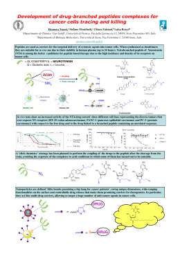
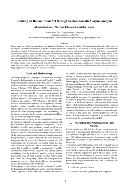
Mechanical behavior of glass-filled epoxy resins:
experiments, homogenization methods for
syntactic foams, and applications
Tesi presentata per il
conseguimento del titolo di Dottore di Ricerca
Dottorato in Materiali per l’Ingegneria — XIII Ciclo
Università degli Studi di Brescia
Dipartimento di Ingegneria Civile
di
Lorenzo Bardella
Dicembre 2000
Relatore:
Prof. Francesco Genna
Collegio dei Docenti
del Dottorato in Materiali per l’Ingegneria
dell’Università degli Studi di Brescia
Prof. A.
Prof. L.E.
Prof. A.
Prof. G.
Dott. G.
Prof. F.
Prof. M.G.
Dott. I.
Dott. M.
Prof. G.
Prof. R.
Dott. L.
Prof. G.
Prof. L.
Carini
Depero
D’Amore
Donzella
Faglia
Genna
La Vecchia
Natali Sora
Penco
Plizzari
Roberti
Sartore
Sberveglieri (Coordinatore)
Zavanella
Acknowledgments
Thanks are due to Professor Ezio Tempesti, formerly of the Department of Chemistry and
Physics for Engineering and for Materials of the University of Brescia, for allowing access
to the Applied Chemistry Laboratory and for providing the raw materials for experiments;
to Professors Roberto Contro and Riccardo Pietrabissa for granting the use of the Laboratory of Biological Structure Mechanics of the Politecnico of Milano; to Professor Giorgio
Donzella for allowing access to the Laboratory for Tests on Materials of the Department
of Mechanical Engineering of the University of Brescia.
The author is indebted to Professor Francesco Genna for his invaluable guidance.
Dr. Michel Palumbo is gratefully acknowledged for his fundamental help in what
concerned the material production.
Dr. Maria Prandini deserves my gratitude for her irreplaceable work in the parameter
identification of the epoxy resin model.
Acknowledgments to Mr. Luca Martinelli, Dr. Virginio Quaglini, and Mr. Modestino
Savoia for their assistance in the experimental work, to Mr. Leonardo Lauri for his help
with the Scanning Electron Microscope, and to Mr. Gianmarco Calò, Mr. Alessandro
Gamba, Mr. Ivan Guizzetti, Mr. Sergio Marini, and Mr. Gabriele Samuelli, who were
involved in the present research during the preparation of their Laurea theses ([33], [49],
and [103]).
Furthermore, the author wishes to thank anyone else who somehow helped to accomplish this work (and anybody tells you they helped, probably did).
The Finite Element code ABAQUS has been run at the Department of Civil Engineering, University of Brescia, Italy, under an academic license.
Finally, since some things are better left unsaid, let me just deeply thank anyone who
supported this work through either love or friendship.
v
Sommario
Questa tesi si occupa principalmente dello studio del comportamento meccanico di materiali eterogenei costituiti da un aggregato in sfere cave di vetro (filler) disperso in una
matrice in resina epossidica (binder). Questa morfologia è caratteristica di compositi chiamati schiume sintattiche, i cui singoli componenti omogenei (fasi), in genere, possono
essere costituiti da qualsiasi materiale che soddisfi certi requisiti tecnologici. L’uso di un
filler in vetro e una matrice in resina epossidica è comunque la scelta più comune, in quanto
permette sia di ottenere schiume sintattiche con buone proprietà (macroscopiche) finali,
sia di soddisfare al meglio i requisiti tecnologici per la produzione di tali compositi.
L’obiettivo di questa ricerca è lo sviluppo strumenti analitici in grado di predire il
comportamento meccanico di schiume sintattiche, materiali sempre più utilizzati nella
pratica ingegneristica, ma che a tutt’oggi vengono ancora progettati in base all’esperienza
o a regole empiriche.
Al fine di ottenere modelli dipendenti dalle caratteristiche meccaniche e geometriche
delle varie fasi, si è scelto di seguire un approccio micromeccanico basato sulla teoria dell’omogeneizzazione. Tale approccio, se da un lato permette di ottenere strumenti utili alla
progettazione di materiali compositi, dall’altro, per essere seguito, richiede la conoscenza
del legame costitutivo di ciascuna fase. In questa ricerca, il comportamento meccanico
del vetro è stato sempre assunto elastico lineare fino a rottura, mentre si è appositamente
sviluppato un legame costitutivo per descrivere il comportamento meccanico di resine
epossidiche, per le quali non sembrano essere disponibili strumenti di calcolo adeguati per
predirne il comportamento meccanico, nonostante si tratti materiali vastamente impiegati
nell’ingegneria.
I principali argomenti trattati nella presente tesi possono essere riassunti
1. in una parte sperimentale, consistente nella produzione di provini sia di resine epossidiche che di schiume sintattiche e nelle prove meccaniche degli stessi;
2. nello sviluppo di una tecnica di omogeneizzazione capace di stimare accuratamente
i moduli elastici di schiume sintattiche per un ampio spettro di parametri caratterizzanti le fasi costituenti;
3. nella validazione di questa tecnica di omogeneizzazione e nella sua applicazione alla
progettazione di materiali compositi;
4. nello sviluppo di un legame costitutivo per resine epossidiche;
5. nell’analisi micromeccanica di schiume sintattiche in regime non lineare e anelastico.
vii
Il primo punto costituisce la prima parte della tesi, in cui è inclusa la descrizione di come
i materiali testati per questa ricerca sono stati prodotti. I punti 2 e 3 sono trattati nella
seconda parte di questa dissertazione, dedicata all’omogeneizzazione in campo elastico
lineare. Infine, la terza parte della tesi si occupa degli ultimi due argomenti, essendo rivolta
allo studio del comportamento oltre il campo elastico e lineare dei materiali studiati.
La tecnica di omogeneizzazione in campo elastico lineare è stata sviluppata in modo tale
da essere in grado di predire accuratamente le costanti elastiche di schiume sintattiche (i)
constituite da fasi isotrope, (ii) il cui filler sia composto da sfere cave di diverse dimensioni,
densità ed eventualmente materiale e (iii) in cui siano restate imprigionate bolle d’aria nella
matrice a causa delle modalità di produzione.
Come esempio di applicazione a un problema ingegneristico, tale tecnica di omogeneizzazione è stata utilizzata per la progettazione ottima di pannelli sandwich non convenzionali, impiegati nell’industria navale per la fabbricazione di scafi. Tali sandwich sono
costituiti da lastre di resina fibrorinforzata tra loro interconnesse e suddivise da un cuore in
schiuma sintattica. L’obiettivo della progettazione è consistito nell’ottenere, sotto vincoli
dettati da considerazioni tecnologiche, il sandwich più leggero che soddisfasse un ulteriore
vincolo sulla sua rigidezza globale.
Il legame costitutivo per le resine epossidiche è stato sviluppato con il fine di descriverne il comportamento meccanico, sia ciclico che viscoso, nello stato vetroso e prima
che la loro resistenza massima sia raggiunta. Le prove meccaniche hanno dimostrato che
in tale regime deformativo le resine epossidiche esibiscono un comportamento prevalentemente viscoelastico non lineare. Tale modello è stato impiegato per studiare, attraverso
simulazioni numeriche agli Elementi Finiti, il comportamento meccanico oltre il limite
elastico lineare di schiume sintattiche.
L’omogeneizzazione analitica del comportamento meccanico di schiume sintattiche in
regime non lineare e anelastico è stata basata su un legame semplificato per le resine
epossidiche e sull’approntata tecnica di omogeneizzazione dei moduli elastici. L’estensione
di tale tecnica al campo non lineare e anelastico è stata condotta sia tramite metodi
noti di letteratura, sia attraverso lo sviluppo di un nuovo metodo di omogeneizzazione
specificatamente sviluppato per schiume sintattiche.
I risultati ottenuti in questa ricerca sono stati parzialmente pubblicati, in forma generalmente più compatta, in [12], [13], [11], [9], [10], [15], [14], [98] e [16].
Summary
This thesis is mainly concerned with the investigation of the mechanical behavior of heterogeneous materials made up of glassy hollow spheres dispersed into an epoxy resin matrix.
This peculiar composite morphology characterizes the so-called syntactic foams, whose
phases can in general be constituted by any homogeneous material which meets proper
technological specifications. However, the use of both glassy fillers and epoxy binders is
the most common because this choice allows one to both obtain good properties for the
final composite and best satisfy the technological requirements in the manufacturing stage.
The key goal of this research consists of providing analytical tools able to predict the
mechanical behavior of such composites, which are being increasingly employed in the
engineering practice, but still designed by means of rules of thumb. A micromechanical approach based on the homogenization theory has been followed, in order to obtain
constitutive laws based on both geometrical and mechanical data of the phases.
Since the homogenization approach requires the knowledge of the constitutive laws of
all the phases, the mechanical behavior of epoxy resins, interesting engineering materials
in themselves and apparently not much studied in their glassy state, has been investigated
as well.
The research herein reported involves the following steps:
1. performing experimental tests on both epoxy resins and syntactic foams in order to
both get an insight into their mechanical behaviors and make results available to
validate the analytical models;
2. the development of a linear elastic homogenization procedure able to accurately estimate the elastic moduli of syntactic foams for a wide range of constituent parameters;
3. the verification of the capability of such a homogenization method to design syntactic
foams in the linear elastic range;
4. the development of a constitutive law for epoxy resins;
5. the micromechanical analysis of the syntactic foams behavior beyond the linear elastic range.
The first point is embodied in the first part of the thesis which also includes the description
of the production modalities of both the epoxy resins and the syntactic foams tested
for this research. Both the second and third points are treated in the second part of
this dissertation, concerned with the homogenization methods in the linear elastic range.
Finally, the third part of this thesis deals with the last two points and, in general, with
the analysis of nonlinear and inelastic effects on the studied materials.
ix
The linear elastic homogenization procedure has been developed to be suitable for
syntactic foams (i) made up of isotropic phases, (ii) whose filler can be constituted by
graded hollow spheres, possibly of different (isotropic) materials, and (iii) in which the
imperfect vacuum manufacturing has left adventitious air bubbles entrapped in the matrix.
As an engineering application example, this model has been employed for the optimum
elastic design of syntactic foamed sandwich panels used in the naval industry.
The constitutive law for epoxy resins has been developed in order to describe their
behavior before the material strength is reached, which has been shown, through the
experimental tests, to be mainly nonlinear viscoelastic. Such a constitutive model is
needed to investigate the nonlinear and inelastic behavior of syntactic foams constituted
by glassy fillers into epoxy matrixes, by means of a numerical homogenization based on
Finite Element analyses.
The analytical homogenization of the syntactic foam behavior beyond the linear elastic
range has been based on both the here developed linear elastic homogenization procedure
and a simplified constitutive law for epoxy resins. The nonlinear and inelastic effects have
been accounted for by both exploiting suitable literature theories and developing an ad
hoc nonlinear homogenization scheme.
Part of the results obtained in this research has been published in a usually more
compact form in [12], [13], [11], [9], [10], [15], [14], [98], and [16].
Contents
Acknowledgments
v
Sommario
vii
Summary
ix
Notation
xv
1 Introduction
1
I
5
Experimental results
2 Material preparation
7
2.1 Production of epoxy resin and syntactic foam . . . . . . . . . . . . . . . . . 7
2.2 Geometry and instrumentation of the specimens . . . . . . . . . . . . . . . 12
3 Epoxy resins: experimental results
17
3.1 Introduction . . . . . . . . . . . . . . . . . . . . . . . . . . . . . . . . . . . . 17
3.2 Epoxy resin DGEBA DER 332 cured with the hardener DDM 32950 . . . . 18
3.3 Epoxy resin SP Ampreg 20T M cured with UltraSlow Hardener . . . . . . . 23
4 Syntactic foams: experimental
4.1 Syntactic foam type 1 . . . .
4.2 Syntactic foam type 2 . . . .
4.3 Syntactic foam type 3 . . . .
4.4 Syntactic foam type 4 . . . .
4.5 Syntactic foam type 5 . . . .
4.6 Syntactic foam type 6 . . . .
II
results
. . . . .
. . . . .
. . . . .
. . . . .
. . . . .
. . . . .
Linear elastic behavior
.
.
.
.
.
.
.
.
.
.
.
.
.
.
.
.
.
.
.
.
.
.
.
.
.
.
.
.
.
.
.
.
.
.
.
.
.
.
.
.
.
.
.
.
.
.
.
.
.
.
.
.
.
.
.
.
.
.
.
.
.
.
.
.
.
.
.
.
.
.
.
.
.
.
.
.
.
.
.
.
.
.
.
.
.
.
.
.
.
.
.
.
.
.
.
.
.
.
.
.
.
.
.
.
.
.
.
.
.
.
.
.
.
.
.
.
.
.
.
.
.
.
.
.
.
.
55
55
62
63
65
66
67
101
5 Introduction
103
5.1 Overview . . . . . . . . . . . . . . . . . . . . . . . . . . . . . . . . . . . . . 103
5.2 Summary . . . . . . . . . . . . . . . . . . . . . . . . . . . . . . . . . . . . . 104
xi
6 Review of some linear homogenization methods
6.1 General definitions . . . . . . . . . . . . . . . . . . . . . .
6.2 The Eshelby solution . . . . . . . . . . . . . . . . . . . . .
6.3 The dilute approximation . . . . . . . . . . . . . . . . . .
6.4 The Voigt and Reuss bounds . . . . . . . . . . . . . . . .
6.5 The Hashin–Shtrikman bounds . . . . . . . . . . . . . . .
6.5.1 The Hashin–Shtrikman bounds for syntactic foams
6.6 The Mori–Tanaka Method . . . . . . . . . . . . . . . . . .
6.6.1 The Mori–Tanaka estimate for syntactic foams . .
6.7 The Self–Consistent Scheme . . . . . . . . . . . . . . . . .
6.7.1 The Self–Consistent estimate for syntactic foams .
6.8 Other methods and further extensions . . . . . . . . . . .
.
.
.
.
.
.
.
.
.
.
.
.
.
.
.
.
.
.
.
.
.
.
.
.
.
.
.
.
.
.
.
.
.
.
.
.
.
.
.
.
.
.
.
.
.
.
.
.
.
.
.
.
.
.
.
.
.
.
.
.
.
.
.
.
.
.
.
.
.
.
.
.
.
.
.
.
.
.
.
.
.
.
.
.
.
.
.
.
.
.
.
.
.
.
.
.
.
.
.
107
. 107
. 112
. 114
. 114
. 114
. 115
. 116
. 117
. 117
. 118
. 119
7 Analytical derivation of the effective moduli of syntactic foams with
graded filler and “unwanted” voids
121
7.1 Introduction to the chosen homogenization approach . . . . . . . . . . . . . 121
7.2 The shear modulus derivation for the case in which the RVE is made by
one composite sphere type only . . . . . . . . . . . . . . . . . . . . . . . . . 123
7.3 The bulk modulus derivation for the case in which the RVE is made by one
composite sphere type only . . . . . . . . . . . . . . . . . . . . . . . . . . . 131
7.4 Extension to consider both the filler gradation and the presence of “unwanted” voids . . . . . . . . . . . . . . . . . . . . . . . . . . . . . . . . . . . 133
Appendixes to Chapter 7
7.A Discussion of the sequential homogenization technique proposed by Nielsen
[91] . . . . . . . . . . . . . . . . . . . . . . . . . . . . . . . . . . . . . . . .
7.B The coefficients of equation (7.2.33) . . . . . . . . . . . . . . . . . . . . .
7.C An alternative approach for the derivation of the Mori–Tanaka “composite
sphere”–based estimate . . . . . . . . . . . . . . . . . . . . . . . . . . . .
7.D Dimensionless abaci to homogenize voids into a matrix: application to syntactic foams . . . . . . . . . . . . . . . . . . . . . . . . . . . . . . . . . . .
137
. 137
. 140
. 143
. 147
8 Comparison between reference experimental results and analytical estimates
153
8.1 The Huang and Gibson results . . . . . . . . . . . . . . . . . . . . . . . . . 153
8.2 The Kinra and Ker results . . . . . . . . . . . . . . . . . . . . . . . . . . . . 157
9 Comparison between our experimental results
9.1 Introduction . . . . . . . . . . . . . . . . . . . .
9.2 Syntactic foam type 1 . . . . . . . . . . . . . .
9.3 Syntactic foam type 2 . . . . . . . . . . . . . .
9.4 Syntactic foam type 3 . . . . . . . . . . . . . .
9.5 Syntactic foam type 4 . . . . . . . . . . . . . .
9.6 Syntactic foam type 5 . . . . . . . . . . . . . .
9.7 Syntactic foam type 6 . . . . . . . . . . . . . .
10 Influence of the filler gradation
and analytical estimates161
. . . . . . . . . . . . . . . . 161
. . . . . . . . . . . . . . . . 162
. . . . . . . . . . . . . . . . 162
. . . . . . . . . . . . . . . . 163
. . . . . . . . . . . . . . . . 164
. . . . . . . . . . . . . . . . 164
. . . . . . . . . . . . . . . . 166
167
11 Comparison between predictions of numerical simulations and analytical
estimates
173
12 An application: the elastic design of syntactic foamed sandwiches obtained by filling of three-dimensional sandwich-fabric panels
181
12.1 Introduction . . . . . . . . . . . . . . . . . . . . . . . . . . . . . . . . . . . . 181
12.2 Elastic stiffness of a symmetric sandwich beam . . . . . . . . . . . . . . . . 183
12.3 Homogenization of the syntactic foam . . . . . . . . . . . . . . . . . . . . . 189
12.4 Homogenization of the fiber-reinforced resin and of the sandwich core . . . 191
12.5 Verification of the sandwich model by comparison with experimental results 195
12.6 Design of minimum weight panels . . . . . . . . . . . . . . . . . . . . . . . . 199
12.7 Open issues and conclusions . . . . . . . . . . . . . . . . . . . . . . . . . . . 211
13 Effective thermal expansion coefficient
213
III
217
Inelastic and nonlinear behavior
14 Introduction
219
15 Linear viscoelastic matrix
221
16 A phenomenological constitutive law for the nonlinear viscoelastic behavior of epoxy resins in the glassy state
225
16.1 Introduction . . . . . . . . . . . . . . . . . . . . . . . . . . . . . . . . . . . . 225
16.2 Constitutive law derivation . . . . . . . . . . . . . . . . . . . . . . . . . . . 226
16.3 Comments on other literature constitutive models involving the Eyring
equation . . . . . . . . . . . . . . . . . . . . . . . . . . . . . . . . . . . . . . 232
16.4 Material parameters identification and comparison with experimental results 235
16.5 Three-dimensional implementation . . . . . . . . . . . . . . . . . . . . . . . 239
16.6 Application to syntactic foams . . . . . . . . . . . . . . . . . . . . . . . . . 240
16.7 Open issues and conclusions . . . . . . . . . . . . . . . . . . . . . . . . . . . 241
17 Review of some nonlinear homogenization methods
17.1 Introduction . . . . . . . . . . . . . . . . . . . . . . . . . .
17.2 The Incremental, Secant, and Modified Secant methods .
17.2.1 Approach philosophy . . . . . . . . . . . . . . . . .
17.2.2 The Incremental Method . . . . . . . . . . . . . .
17.2.3 The Secant Method . . . . . . . . . . . . . . . . .
17.2.4 The Modified Secant Method . . . . . . . . . . . .
17.2.5 Particularization to the J2 –flow theory of plasticity
17.3 Variational methods for nonlinear composites . . . . . . .
17.3.1 Behavior of the phases and basic results . . . . . .
17.3.2 The Talbot and Willis variational principle . . . .
17.3.3 The Ponte Castañeda variational principle . . . . .
17.4 Transformation Field Analysis . . . . . . . . . . . . . . . .
17.5 Other nonlinear homogenization methods . . . . . . . . .
.
.
.
.
.
.
.
.
.
.
.
.
.
.
.
.
.
.
.
.
.
.
.
.
.
.
.
.
.
.
.
.
.
.
.
.
.
.
.
.
.
.
.
.
.
.
.
.
.
.
.
.
.
.
.
.
.
.
.
.
.
.
.
.
.
.
.
.
.
.
.
.
.
.
.
.
.
.
.
.
.
.
.
.
.
.
.
.
.
.
.
.
.
.
.
.
.
.
.
.
.
.
.
.
.
.
.
.
.
.
.
.
.
.
.
.
.
.
.
.
.
.
.
.
.
.
.
.
.
.
245
245
245
245
247
248
248
251
252
252
254
256
259
261
17.5.1 A method based on the Fast Fourier Transform . . . . . . . . . . . . 261
17.5.2 An approximate method for particulate composites made up of a
linear elastic filler into a nonlinear matrix . . . . . . . . . . . . . . . 261
18 Homogenization of the syntactic foam inelastic and nonlinear behavior 265
18.1 Introduction . . . . . . . . . . . . . . . . . . . . . . . . . . . . . . . . . . . . 265
18.2 The Second Order Secant Method . . . . . . . . . . . . . . . . . . . . . . . 266
18.2.1 The Second Order Secant Method for syntactic foams . . . . . . . . 266
18.3 Application of the Incremental, Secant, Second Order Secant, and Modified
Secant methods to syntactic foams . . . . . . . . . . . . . . . . . . . . . . . 269
19 Closure
279
19.1 Conclusions . . . . . . . . . . . . . . . . . . . . . . . . . . . . . . . . . . . . 279
19.2 Open issues . . . . . . . . . . . . . . . . . . . . . . . . . . . . . . . . . . . . 280
Bibliography
285
Notation
An indicial notation will be adopted to indicate tensors with the following exceptions,
for which boldface letters will be used: (i) the case in which tensors are used as implicit
independent variables of a function (e.g., σij = fij (ε)), (ii) the formalism needed to express
the appurtenance of a tensor to a set (e.g., x ∈ Γ), and (iii) when tensors
are usedoto
n
indicate independent functions in variational problems (e.g., u(σ) = supε σij εij − w(ε) ).
We shall adopt lower case letters to indicate vectors and second-order tensors if they
are referred to microscopic quantities, otherwise (i.e., for any tensor indicating macroscopic
quantities and for higher order tensors) capital letters will be employed.
xv
Chapter 1
Introduction
Syntactic foams (the first term coming from the Greek meaning “the placing of parts
in a certain order”) are heterogeneous materials classifiable as particulate composites.
This class of composites consists of materials made up of an aggregate, constituted by
discrete particles approximately spherically shaped, embedded into a continuous phase,
the so-called matrix or binder. From the morphological viewpoint, these heterogeneous
materials are distinguished from the fiber-reinforced composites (in which the presence
of fibers aligned along preferential directions usually gives high mechanical properties in
those directions), from the interpenetrating network composites, made by two or more
continuous phases, and from the granular composites, such as polycrystals, in which a
continuous phase does not exist.
Syntactic foams are obtained by filling a polymeric matrix with a gas-filled aggregate
usually consisting of hollow spherical inclusions. In most of the applications the matrix
is made by an epoxy resin, that gives to the composite good temperature resistance since
it maintains high stiffness at elevated temperatures, and the aggregate is constituted by
glass, that contributes to the dimensional stability of these materials (i.e., they have low
coefficient of thermal expansion over a wide temperature range).
In recent years, syntactic foams have been employed in many engineering applications,
ranging from aerospace plug manufacturing to ablative heat shields for re-entry vehicles,
underwater buoyancy aids, and, more recently, structural components such as hulls and
bulkheads of ships and submarines; in these last cases syntactic foams have been employed
also as the core materials of sandwiches. Besides, syntactic foams are also used as putties
for fixing hydraulic structures and in the naval industry.
These applications often exploit several features typical of syntactic foams, beside the
high specific mechanical properties (defined by the ratios between the values of the mechanical properties and the material density), such as the low dielectric constant value,
the good ablation behavior, the good match to acoustic impedance of water (for sonar
applications), and the good thermal and water insulation properties. One of the most exploited specific mechanical properties in naval engineering is the capability of withstanding
considerable hydrostatic pressure. Moreover, the hollow filler allows the final material to
have lower residual stresses than particulate composites filled with solid particles [104].
The use of syntactic materials as plug assist tooling, replacing conventional materials
such as aluminum, wood, or felt, has become increasingly popular in the thermoforming
industry; indeed, the low thermal conductivity and the low specific heat translate to
1
2
Chapter 1 — Introduction
lower heat transfer which reduces warmup time and virtually climates material sticking
to the plug. Typical applications in this field are on sheet-fed, rotary, or in-line machines;
syntactic foams may be used with most commonly thermoformed materials, as well as
some of the most exotic materials available today.
Furthermore, there is interest in employing syntactic foams for biomedical applications
such as the core of artificial limbs or prostheses.
Syntactic foams are preferred to standard foams (containing blown gas bubbles only)
when high specific mechanical properties are required, rather then just low density. Moreover, standard foams have the voids completely, or at least partly, connected to each other
(reason for which they are often considered as interpenetrating network composites), feature that makes them difficult to use for underwater applications; on the contrary, syntactic
foams show very low water absorption. Standard foams may become preferable because
they can be produced at very low densities, unlike syntactic foams for which densities less
than 0.1 g/cm3 are almost impossible to achieve, assuming the absence of adventitious air
bubbles entrapped in the matrix (vacuum manufacturing).
A comprehensive review of the technological research on syntactic foams until the mid
eighties can be found in Shutov [104], where, by the way, many papers are quoted about
the use of syntactic foams in naval, industrial, aerospace, and civil engineering.
For an optimal structural design, there is the need, for instance to allow numerical
simulations on Finite Element codes, of developing constitutive models able to describe
the material behavior of syntactic foams.
If such models are developed by means of a suitable micromechanical approach, they
result, unlike the macroscopic phenomenological models, to be functions of the mechanical
and geometrical data of the composite phases. This desirable feature allows one to even
design the best composite for a given engineering application. Without the knowledge of
such a constitutive model, the composite design may be a very expensive trial and error
procedure which may even not lead to the best possible result. For instance, in the case of
syntactic foams, after having decided the materials to be employed as matrix and hollow
spheres, it is important to choose both the filler volume fraction and its gas content (which
affects the particle density).
As far as we know, the constitutive modeling of syntactic foams is a rather unexplored
area (see, for instance, the methods reviewed in [104], mostly either heuristic or based on
unreal assumptions). Even the computation of the so-called effective (i.e., macroscopic)
elastic moduli of such composites can be difficult if standard homogenization techniques
(i.e., methods developed in order to link the microscopic and macroscopic composite behaviors) are employed; indeed, the presence of a void phase causes a poor behavior of
methods which cannot properly take the connectedness of the matrix into account. Such
a problem directly translates into the nonlinear range, whose description is even made
more difficult by the dependence of the syntactic foam behavior on the constitutive laws
of the phases. In fact, owing to the polymeric nature of the matrix, the prediction of the
binder behavior itself may constitute a problem.
In this thesis, we shall focus on syntactic foams whose matrixes are made up of epoxy
resins, which are known to be the best binders for syntactic foams [104] and are by themselves interesting materials for engineering.
Epoxy resins are being widely employed for structural applications, mostly when there
is the need of connecting structural elements made up of different materials; for instance,
Chapter 1 — Introduction
3
they are used to anchor steel bars into concrete (concrete joints) or timber (composite
beams).
The use of epoxy resins as matrixes of both particulate and fiber-reinforced composite
materials is anyway one of the most important applications in engineering; one meaningful
and interesting instance is that already cited of sandwich panels filled with syntactic foam,
in which the skins consist of fiber-reinforced epoxy resins. These sandwiches are being
employed with increasing frequency in naval engineering applications when weight, water
absorption, and strength are critical issues.
In all the above mentioned applications, epoxy resins are subjected to high stress
gradients. To design such kinds of (micro)structures it is then definitely necessary to be
able to predict how the stress and strain fields develop over these materials.
The subject of this dissertation is the development of constitutive models for epoxy
resins and syntactic foams.
These materials have shown in laboratory tests to have very limited ductility at room
temperature. In particular, syntactic foams filled with high volume fractions of glass
hollow spheres, which are the most interesting for engineering applications, have exhibited
a behavior nearly elastic-brittle and failed in compression at a deformation of the order of
5%. Therefore, all the studied models have been developed under the assumption of small
strains.
The first step of this work has consisted in the preparation, instrumentation, and
mechanical testing of a reasonably wide range of both epoxy resins and syntactic foams.
Such a step has been necessary to get an insight into the mechanical behavior of these
materials, whose experimental behavior, specially for the composites, is quite scarcely
documented in the literature. Furthermore, the industrial nature of the epoxy resin batches
makes different batches have slightly different properties. Therefore, it has been judged
essential to produce and test also the plain epoxy resins used as matrixes for the syntactic
foams.
In this thesis, we shall furnish an homogenization technique able to accurately predict
the elastic constants of any syntactic foam whose final density, filler gradation, and filler
volume fraction are known beside the elastic moduli of the phases.
As an example of engineering application of such a model, we shall make ready an
optimum design procedure for syntactic foamed sandwiches in the linear elastic range;
the goal of this optimization is of designing, under some technological constraints, the
lightest sandwich whose stiffness is prescribed. To this purpose, we shall also propose an
approximate but accurate method to evaluate the shear stiffness of sandwich beams.
For what the behavior beyond the linear elastic range is concerned, we shall both derive
a model able to describe the nonlinear viscoelastic behavior of epoxy resins in the glassy
state and propose models to estimate the nonlinear and inelastic behavior of syntactic
foams, again by means of a homogenization approach.
The predictions of all the proposed models will be compared (i) with reference experimental results, (ii) with the new experimental results obtained in the course of this work,
and (iii) with the results of numerical simulations.
4
Chapter 1 — Introduction
Part I
Experimental results
5
Chapter 2
Material preparation
In this chapter, we report the production modalities of the specimens tested by us together
with the description of how the mechanical behavior of different syntactic foams has been
experimentally characterized.
Two different epoxy resins have been employed as matrixes for making different syntactic foams. Specimens of plain epoxy resins were also tested to characterize the matrix
behavior.
The specimens were produced at both the Applied Chemistry Laboratory and the
Mechanical Engineering Laboratory of the Faculty of Engineering of the University of
Brescia.
Part of this chapter has already been published in [9].
2.1
Production of epoxy resin and syntactic foam
To obtain a syntactic foam there is the need of mixing two components: the matrix (also
called binder) and the hollow spheres (i.e., the filler). For the syntactic foams produced
by us, the matrix has always been constituted by an epoxy resin and the filler by hollow
microspheres (i.e., hollow spheres whose outer radius is less than 100 µm). The binder
is in turn constituted by a pure resin (epoxy prepolymer) and a hardener (or curing
agent), which allows chemical bonds to arise among the molecules of the prepolymer in
the so-called “curing” process. Different types of pure epoxy resins and curing agents have
been mixed obtaining different matrixes and then different types of syntactic foams. The
prepolymers employed in this research are:
• epoxy resin DGEBA (diglycidyl ether of bisphenol A), produced by Dow Chemicals
under the name DER 332;
• epoxy resin SP Ampreg 20T M , produced by SP Systems, Montecatini Advanced
Materials,
and the curing agents are:
• hardener DDM 32950, produced by Fluka (always used to cure the epoxy resin
DGEBA DER 332);
7
8
Part I — Experimental results
• hardener Laromin C252, produced by BASF (used only once, in conjunction with
the epoxy resin DGEBA DER 332, to make a syntactic foam: see section 4.2);
• curing agent “UltraSlow Hardener”, produced by SP Systems, Montecatini Advanced
Materials (always employed to harden the epoxy resin SP Ampreg 20T M ).
Since all these components are usually preserved in a state incompatible with the mixing
operation, they need a preparation to be mixed.
At room conditions the hardener DDM 32950 is in a granular state; since its melting
temperature is 92.5◦ C (Celsius degrees), we had to warm it up to 120◦ C on an electric
plate (see figure 2.1) to make it liquid as fast as possible without getting into oxidization
problems.
Figure 2.1: The hardener melting
The prepolymer DGEBA DER 332 is instead preserved at the temperature of −18◦ C
to avoid secondary polymerization reactions; at this temperature it is in a crystallized
state. To make it possible to mix it with the curing agent it is necessary to warm also the
pure resin up to the temperature of 60◦ C.
Chapter 2 — Material preparation
9
The preparation of both the resin SP Ampreg 20T M and the UltraSlow Hardener is
instead trivial, because at the room temperature both of them are in a liquid state.
When both the curing agent and the epoxy prepolymer are liquid, the stoichiometric
amount of the former has to be transferred in the beaker containing the latter, which in
turn is laid on a technical balance to check the amount of hardener decanted. This last
expedient is essential because the amount of hardener to be melted before the decanting
must be more than that strictly stoichiometric; indeed, in the decanting process an amount
of curing agent that can not be quantified gets lost for crystallization in the contact with
the top of the beaker, cooler than its bottom (which has a temperature of ≈ 120◦ C). This
operation has then to be done as fast as possible, to avoid to lose too much hardener, and
carefully, to be sure to transfer the right amount of curing agent into the beaker containing
the pure resin (see figure 2.2).
The obtained mixture has to be stirred by hand with a glass rod until the filaments
visible to the naked eye, due to the contact of hardener and prepolymer, disappear; usually
this last process takes more or less 5 minutes. The glass rod is in turn warmed up at 60◦ C
to avoid thermal shocks that would inhibit the curing. If just plain epoxy resin specimens
Figure 2.2: The decanting operation
have to be produced, at this point one can decant the mixture in the moulds. The moulds
have to be internally spreaded with silicone to allow the specimens extraction after the
material hardens. After the dies are filled with the resin, they must be left in an oven
to allow the curing process, for a time and at a temperature dependent upon the resin
itself. The epoxy resin DGEBA DER 332, cured with the hardener DDM 32950, needs
to be kept in the oven for 24 hours at the temperature of 60◦ C; instead, to cure the
10
Part I — Experimental results
epoxy resin SP Ampreg 20T M with UltraSlow Hardener there is the need to leave it in the
oven for 24 hours at the temperature of 30◦ C, then for 16 more hours at the temperature
of 50◦ C. These long times can be explained by considering that the curing process is
highly exothermic; indeed, the stabilized glass transition temperature, Tg , of the epoxy
resin DGEBA DER 332 hardened with the DDM 32950, is of about Tg ≈ 170◦ C and
its curing reaction easily brings the temperature of the specimens to more than 200◦ C:
this means that the specimens have to be kept in the oven for a long time to cool them
down (at 60◦ C) to avoid thermal shocks when they are removed from the oven. This last
observation makes it clear that the choice between different prepolymers and hardeners
is also dependent upon the easiness of keeping the exothermy of the curing process under
control, in particular when operating with large amounts of material. Furthermore, the
moulds have to be designed in such a way as to allow the resin to maintain its highest
curing temperature for the longest possible time: this allows the resin to reach an actual
glass transition temperature close to its stabilized value. To this purpose the moulds
should be designed large enough to contain an amount of resin such that it can stay as
warm as possible for a long time; the whole process of finding the conditions for having an
efficient curing stage is empiric and the quality of the obtained resin can be a posteriori
checked by measuring its actual glass transition temperature by means of a Differential
Stream Calorimeter (DSC). Note that the resin SP Ampreg 20T M needs a two step curing
process, because the hardener UltraSlow is actually a mixture of different curing agents
which react at different temperatures.
We produced two, in principle different, kinds of epoxy resins, both made by the
prepolymer DGEBA DER 332 cured with the hardener DDM 32950. This is because a
few specimens of this epoxy resin have also been postcured at 180◦ C to be sure to stabilize
their glass transition temperature, i.e., to build the maximum number of crosslinks between
the prepolymer and the curing agent, number dependent upon the stoichiometry and the
random topology of the mixture; indeed, although the epoxy prepolymer and the hardener
are stoichiometrically mixed, it is not obvious at all that all the molecules get the chance
to build all the chemical bonds they theoretically could, because of the random relative
position between the prepolymer and the curing agent molecules (Oleinik, [92]).
Independently upon the constituents, any resin has to be degassed in the first half hour
of the curing process; to do that the oven is connected with a vacuum pump.
To produce syntactic foam specimens, the filler has to be added to the not yet hardened
epoxy resin. This operation is not trivial at all, by the way being dependent upon the
wanted volume fraction of filler f in the composite. If the filler volume fraction is less
than ≈ 50% there is the need to use a “traditional” technique, characterized by mixing
at various stages, by hand and mechanically, the binder and the filler; on the contrary, if
the maximum content of filler compatible with its granulometry is the goal, one can not
use the “traditional” technique owing to the high viscosity that the slurry would have,
but it is necessary to employ the so-called “injection” technique, in which the binder is
directly injected under vacuum in a die filled with hollow microspheres packed as tightly
as possible by means of a vibrator. This last technique (Tempesti, [114]) does not allow
the filler volume fraction to be known in advance before weighing the final specimen;
furthermore, with the “injection” method it is quite difficult to avoid the presence in the
composite of adventitious air bubbles entrapped in the matrix (in the following called
“unwanted” voids, even if in some cases they are on purpose blown in the matrix in order
Chapter 2 — Material preparation
11
to lighten the composite).
Let us now go into more details about the two mixing techniques. The “traditional”
technique consists of mixing the epoxy resin with the filler by transferring the former in
the beaker containing the latter, placed on a technical balance. This decanting process
has to be done very slowly to avoid turbulence which could disperse a significant amount
of microspheres in the air because of their very low density. Note that also the hollow
microspheres need to be warmed up at 60◦ C in order both to avoid thermal shocks in
the resin when mixing them together and to make the slurry as fluid as possible; this is
important because an excessive slurry viscosity could give rise to problems in the mixing
process, with the result of producing a macroscopically inhomogeneous syntactic foam
containing also a large amount of “unwanted” voids.
After mixing by hand with a glassy rod for a few minutes, the slurry becomes homogeneous enough to be put on a reactor thermostated at Tr = 45◦ C, where the foam
is degassed under vacuum and is continuously shaken mechanically (see figure 2.3). The
Figure 2.3: The devices employed with the “traditional” technique: the reactor, the dies,
the vacuum pump, and the oven
temperature Tr must be set coming to an arrangement between the necessity of having a
slurry fluid enough to be mixed and the need of slowing down the curing process as long
as the slurry is not in the dies yet. This phase, lasting at least 90 minutes, needs to be
accomplished very carefully; indeed, because of the large amount of air entrapped in the
syntactic foam during the first shaking process made by hand, the degassing causes the
slurry to inflate owing to the ascensional motion of the air bubbles. This phenomenon
could cause an excessive volumetric increment of the mix which would give rise to the adhesion of a large amount of foam to the top of the reactor, making this portion of material
12
Part I — Experimental results
unavailable for the subsequent transferring in the dies because of the high viscosity of the
slurry. To avoid this problem it is necessary to connect and to disconnect alternately the
vacuum pump to the reactor, allowing the slurry to go back to the bottom of the reactor
when the pump is disconnected after some swelling has been observed. To check the behavior of the slurry under vacuum, a reactor with a plexiglas top, much more capacious
than the amount of the produced syntactic foam, has been designed and used.
Finally, the syntactic foam can be decanted in the moulds, which are also kept under
vacuum until all the slurry is correctly placed into them. The moulds must be internally
spreaded with silicone to allow the specimens extraction after their hardening.
With the “injection” technique the die, in which the filler is placed, must be thermostated like the reactor in the “traditional” technique, to allow the epoxy resin, injected
using a piston system, to fill as much as possible the space left by the hollow microspheres
in the mould; to obtain the best performance in this process the filler can be treated with
plasma, which reduces the filler surface tension. Furthermore, the filler can be silanized
(i.e., subjected to a surface treatment with chemical agents, [114]), in order to build chemical bonds between the glass of the filler and the epoxy resin. All these techniques, designed
both to improve the adhesion between the filler and the matrix and to make the volume
fraction of “unwanted” voids as small as possible, are still under study; the improvement of
the adhesion between glass and epoxy resin should have effects on the nonlinear behavior
of syntactic foams, whereas the presence of “unwanted” voids affects, as it will be shown
in the second part of this thesis, the linear elastic behavior too.
After placing the syntactic foam into the dies, independently on the technique used to
do that, the dies must be left in an oven set at a temperature and for a time dependent
upon the resin employed, as above explained.
2.2
Geometry and instrumentation of the specimens
The Young modulus, the Poisson ratio, and the shear modulus were measured in compressive, tensile, torsional, and cyclic uniaxial tests, for both epoxy resins and syntactic foams;
furthermore, biaxial tests were performed on specimens subjected to combined torsion and
tension or compression to determine, under plane stress conditions, the failure envelope
in its part where the principal stresses have opposite sign. Finally, uniaxial compressive
creep tests were carried out to characterize the epoxy resin viscous behavior.
We produced specimens of different geometries depending on the various testing machines employed. Moreover, the production modalities affected the specimen size.
The compressive tests were accomplished on cylindrical specimens. The “traditional”
technique allowed us to make cylindrical specimens of height h = 100 mm and base
diameter φ = 30 mm; this type of specimen will be in the following labeled as CYL1;
by employing the “injection” technique it was possible to produce specimens of diameter
φ ≈ 20 mm and height h such that h ≈ 3.3φ (CYL2): this smaller specimen was sometimes
employed when the “traditional” technique was adopted also (see section 4.4). All the
compressive tests on the plain epoxy resins were carried out on cylindrical specimens
CYL1, with the exception of the creep tests, for which the height of the specimens was
h = 75 mm instead of 100 mm; this shorter cylinder will be labeled as CYL3.
In the compressive test the barrelling was prevented by inserting thin sheets of Teflon
Chapter 2 — Material preparation
13
between the loading platens and the specimen bases in such a way as to reduce the friction.
In the case in which the composite was made by the “traditional” technique, the
tensile and cyclic tests were performed on dog-bone specimens (later indicated by the
label DB1) whose dimensions are reported on figure 2.4; the dog-bone specimens made
Figure 2.4: DB1 dog-bone specimen geometry (dimensions in mm)
by means of the “injection” are substantially different only in their parts which had to be
gripped, that were turned at a diameter φs ≈ 25 mm instead of 30 mm. The specimen
geometry reported in figure 2.4 was adopted also for the tensile and cyclic tests carried
out on the plain epoxy resin DGEBA DER 332 cured with DDM 32950, whereas for the
same type of tests on the epoxy resin SP Ampreg 20T M cured with UltraSlow Hardener
smaller specimens were employed, characterized by a diameter Rs = 17 mm in the middle
part, where the deformations were measured; they will be in the following called “small
dog-bone” specimens and labeled as DB2.
Finally, for all the tests in which the samples were twisted, dog-bone specimens with
grips of square section were employed, as reported in figure 2.5; we needed this geometry
to make the specimens fit into the torsional testing machine. These specimens, which will
be later denoted by the label DB3, were also adopted to carry out some uniaxial test;
this is because in the last stage of the laboratory experience we tried to get a few failure
envelope points and, for this purpose, we wanted to keep the same specimen geometry
for any stress state (uniaxial or biaxial). The torsional testing machine was the only one
available which allowed us to subject the specimens to a biaxial stress state by twisting
and stretching them simultaneously.
Both the strain gauges and the adhesive used to instrument the specimens are produced
by Hottinger Baldwin Messtechnik.
The syntactic foam specimens were instrumented with strain gauges of the type 1 −
LY 13 − 6/120, which can accurately measure a maximum strain of 5% in both tension and
compression and have measuring grid of dimensions 6 mm × 2.8 mm, nominal resistance
14
Part I — Experimental results
equal to 120 Ω, and a gauge factor of about 2.10 (the precise value of this last datum is
dependent upon the batch). The specimens of plain epoxy resins subjected to tensile or
compressive tests were instrumented with strain gauges of the type 1 − LD20 − 6/120,
which are similar to the strain gauges 1 − LY 13 − 6/120 but can measure strains up
to 10% in both tension and compression. For the torsion tests the strain gauges type
1 − XY 21 − 1.5/120 were employed; they can measure a maximum deformation of 5% and
have measuring grid of dimensions 1.5 mm × 2.5 mm, nominal resistance equal to 120 Ω,
and a gauge factor of about 1.90. All the strain gauges were applied to the specimens by
means of the one–component adhesive Z70.
For each elastic parameter measured, two strain gauges were applied on diametrally
opposite positions on the specimens: this allows us, in the linear elastic range, to compensate measure errors due to the not perfectly centered load application, if it is the case. In
Figure 2.5: DB3 dog-bone specimen geometry (dimensions in mm)
the case of a uniaxial test, the normal Cauchy stress σn has been computed by means of
the relation:
P
(2.2.1)
σn = 2
πr0 (1 + εt )2
in which P is the axial force and r0 is the nominal radius at the point where the transversal
strain εt is recorded.
All the tests were performed at room temperature (≈ 23◦ C) and, with the exception of
the torsion tests and most of those carried out on the small dog-bone specimens, were performed by means of an Instron testing machine (model 1274) at the Laboratory for Tests
on Materials “Pietro Pisa” of the Department of Civil Engineering, University of Brescia.
The load, the displacement, and the strains were usually recorded at a frequency of 3 Hz
Chapter 2 — Material preparation
15
by a data acquisition system implemented by means of the “LabWindows” program. To
check the measures, the applied displacement was recorded twice, using, beside the Instron internal measurement device, a linear voltage displacement transducer (LVDT); for
the compressive tests the force acquisition was checked also, by means of a 10 kN load
cell. All the uniaxial tests were done at a crosshead constant displacement rate variable
from 0.2 mm/min to 10 mm/min; anyway, most of them were performed imposing a
displacement rate of 1 mm/min. The elastic moduli dependence on the displacement rate
will be discussed in chapter 3. Exception was made for the cyclic tests, in which different
cycles were often done at different rates. The dog-bone specimens were gripped using oil
pressure controlled tensile grip fixtures. The only tests accomplished by controlling the
load instead of the displacement were the creep tests.
The Instron testing machine model 8501 of the Laboratory for Tests on Materials of
the Department of Mechanical Engineering, University of Brescia, was used to perform
tests on small dog-bone specimens.
The tests involving torsion were carried out on the MTS testing machine models
319.10.S and 858 Mini Bionix at the Laboratory of Biological Structure Mechanics of
the Politecnico of Milano.
The elastic constants were computed by linear regressions on the set of data and
computed values (e.g., the Cauchy stress) referred to the relevant longitudinal or shear
strain data ranging from 0 to 0.004, regardless of the sign. In the rest of this first,
experimental, part of the thesis, the term “elastic moduli” (referred for instance to the
Young modulus and the Poisson ratio) will mean the measure by linear regression of the
stress–strain slope in the range just defined, taken a priori as linear elastic range. This
assumption will be discussed with respect to phenomena like viscoelasticity which can
affect our measures, in order to try to correctly evaluate the linear elastic constants.
16
Part I — Experimental results
Chapter 3
Epoxy resins: experimental results
3.1
Introduction
This chapter is devoted to reporting the results obtained from the experiments carried out
on specimens of plain epoxy resins. These results have partly been published, in a more
compact form, in [11].
The mechanical characterization of the matrix employed to make a syntactic foam is
obviously a fundamental step in predicting, by means of any kind of microscale approach
(e.g., either theoretical or numerical), the macroscopic behavior of syntactic foams. Even
when syntactic foams are filled with high volume fractions of hollow spheres, there is
the need of having an accurate constitutive law describing the epoxy resin behavior to
understand, for instance, the failure modalities, dependent upon the interaction between
the matrix and the filler. Anyway, for any volume fraction of filler, the determination of the
elastic moduli of the matrix is indispensable for applying any homogenization technique
even in the linear elastic range.
Here, we are first of all interested in determining the elastic moduli. Other material
parameters and features of the epoxy resin behavior, like strength, ductility, hysteretic
behavior, viscosity, and fracture toughness, will be partly investigated by means of uniaxial
tests only, with the exception of a few torsion and Charpy tests. It would obviously be
interesting to investigate the temperature dependence of the mechanical behavior, but this
is beyond the scope of the present work.
The mechanical behavior of several epoxy resins has been characterized, for instance,
in [77] and [82]. These works, however, were mostly concerned with the study of plastic
deformations, which, at least in uniaxial compression, are usually assumed to develop
after the stress–strain curve flattens or reaches a maximum (corresponding to the material
strength which is then assumed to be coincident to the yield stress) [82]. Instead, the tests
here described will most of all focus on the behavior before yielding.
Yamini and Young [135] measured both the Young modulus and the strength of the
epoxy resin DGEBA Epikote 828 produced by Shell cured with various amounts of triethylene tetramine (TETA), in order to find the dependence of measured material parameters
on the resin composition. They found that for given testing conditions (i.e., temperature
and testing rate), both the Young modulus and the strength decrease as the amount of
hardener or the curing temperature are increased. Furthermore, they established that for a
17
18
Part I — Experimental results
given resin composition, both the Young modulus and the yield stress are increasing functions of the testing rate and decreasing functions of the temperature (below Tg ). However,
we shall not discuss the effects of both the curing agent amount and the temperature on
the mechanical properties of the epoxy resins produced by us (as it may appear obvious
owing to what reported in chapter 2).
Note that the industrial nature of the epoxy resin batches causes different batches to
have slightly different properties. This fact, together with the randomness of the curing
process (see section 2.1), made the material parameters of the tested epoxy resins difficult
to be precisely determined.
First (section 3.2), we shall describe the tests on the epoxy resin made by the prepolymer DGEBA DER 332 cured with the hardener DDM 32950 (section 3.2), then (section
3.3) we shall report the experimental results concerning the epoxy resin SP Ampreg 20T M
cured with UltraSlow Hardener (section 3.3).
The matrix of the syntactic foams produced by us (see chapter 4) has always been
chosen between these two kinds of epoxy resins, with one exception only (see section 4.2)
in which the prepolymer DGEBA DER 332 has been cured with the hardener Laromin
C252. We did not test this plain epoxy resin, but it is known that the use of different
hardeners affects the molecular weight between crosslinks and it is typical of thermoset
polymers, as epoxy resins are, that the elastic moduli do not depend upon it (see, for
instance, [92] and [80]). It is instead expected that the viscoelastic behavior and, most of
all, the glass transition temperature Tg are affected from the hardener choice; for instance,
Lee and McKenna, [78], using exactly the same prepolymer but the curing agent Jeffamine
produced by Texaco Chemical Co., found Tg = 42.4◦ C, sensibly less than the value found
for the epoxy here described, Tg ≈ 170◦ C.
3.2
Epoxy resin DGEBA DER 332 cured with the hardener
DDM 32950
This section is concerned with both the regular and the postcured epoxy resin made by
the prepolymer DGEBA DER 332 cured with the hardener DDM 32950 (see section 2.1).
The comparison between the mechanical behavior of the postcured samples and that of
the regular ones will give an idea about the most convenient way of producing this epoxy
resin and, then, syntactic foams made up of it.
Moreover, the aging of this epoxy resin was partly investigated by testing a few specimens one year after their production.
Figures 3.1–3.17 show the results obtained from 26 of the 30 tests carried out on this
resin. Table 3.1 collects all the elastic constants computed from those tests.
In Table 3.1, as well as in the following Table 3.2, the symbol (∗) means that the relevant elastic moduli were measured by a regression over a set of data whose corresponding
maximum absolute value of the longitudinal strain was lower than 0.4%, whereas the ending ng in four sample labels in Table 3.1 means that those tests have not been plotted here
owing to the low accuracy of the recorded data, which, anyway, were as many as needed
to assure nice linear regressions for the elastic constant evaluation. The first column refers
to the shape of the employed specimens (see section 2.2).
Unlike for the tests performed on the epoxy resin SP Ampreg 20T M (which will be
Chapter 3 — Experimental results on the epoxy resins
Sample
1 DB1
1ng DB1
2 CYL1
3 CYL1
5 CYL1
6 CYL1
7 CYL1
8 CYL1
9 DB1
9 DB1
10 DB1
10 DB1
11 DB1
11 DB1
12 DB1
12 DB1
14 DB1
14 DB1
20 CYL1
21 CYL1
22 DB1
23 DB1
23 DB1
2ng DB1
2ng DB1
3ng DB1
3ng DB1
24 DB1
24 DB1
25 DB1
25 DB1
26 CYL1
4ng DB1
E
[M P a]
2856
2886
2814
2924
2836
2809
2992
2857
2895
2576
2927
2550
2767
2675
2884
2894
2871
2849
3231
2513
2882
2826
2760
2898
2851
2863
2754
2808
2556
2826
2596
2802
3017
ν
0.408
0.407
0.404
0.417
0.416
0.413
0.394
0.402
0.464
0.434
0.405
0.409
-
Rate
[mm/min]
0.2
0.1
0.2
1
1
1
1
1
1
0.25
1
0.25
0.25
1
0.25
1
0.25
1
10
10
0.2
0.25
1
0.5
0.125
0.5
0.125
1
0.25
0.25
1
0.1
0.25
Aging
[years]
0
0
0
0
0
1
1
0
0
0
0
0
0
0
0
0
1
1
1
1
0
0
0
0
0
0
0
0
0
0
0
0
0
Stress
State
tens
tens
comp
comp
comp
comp
comp
comp
comp
tens
comp
tens
tens
comp
tens
comp
tens
comp
comp
comp
tens
tens
comp
comp
tens
comp
tens
comp
tens
tens
comp
comp
tens
19
Cycle #
Postcuring
1
1 (*)
1
1
1
1
1
1
1
2
1
2
1
2
1
2
1
2
1
1
1
1
2
1
2
1
2
1
2
1
2
1 (*)
1 (*)
no
no
no
no
no
no
no
no
no
no
no
no
no
no
no
no
no
no
yes
yes
yes
yes
yes
yes
yes
yes
yes
yes
yes
yes
yes
yes
yes
Table 3.1: Elastic moduli computed from displacement–controlled uniaxial tests on epoxy
resin DGEBA DER 332 cured with DDM 32950
20
Part I — Experimental results
reported in section 3.3), we could not record enough data in the initial load ramp of the
creep tests on the epoxy resin DGEBA DER 332 to be able to compute meaningful elastic
constants; therefore, in Table 3.1, samples 15–19 are skipped and, then, only results from
displacement–controlled tests are reported.
From Table 3.1, it is possible to compute the following Young modulus average values:
• compressive Young modulus on the regular (i.e., non-postcured) specimens: Ec =
2861 M P a;
• compressive Young modulus on the postcured specimens: Ec = 2809 M P a;
• tensile Young modulus on the regular specimens: Et = 2770 M P a;
• tensile Young modulus on the postcured specimens: Et = 2816 M P a.
We do not have enough data to discriminate between regular and postcured material in
computing the Poisson ratio; its average value is νt = 0.400 in tension (but we computed
it by averaging of two data only) and νc = 0.410 in compression, without accounting
for the values given by samples 20 and 21, which would make the average value for the
compressive tests equal to νc = 0.417.
Most likely, the large deviation from the average values of both the Young modulus
and the Poisson ratio of samples 20 and 21 is due to the too low frequency at which we
could record the data in those tests; unfortunately, the recorded data have been even
found to be highly scattered. This, together with the high rate of application of the load
(10 mm/min), caused the linear regressions to furnish bad elastic moduli values. This
problem in the data acquisition results in hiding the possible differences between these
“fast tests” and the slower ones which might be affected by viscous effects, even in the
elastic moduli measurement.
Note that the rate, the cycle number, and the aging have not been taken into account
as parameters affecting the elastic moduli measurement in averaging the elastic constant
values collected in Table 3.1; their influence has been neglected for the following reasons.
We could check only a small range of rates; the loading rate does indeed influence the
overall epoxy behavior, but Table 3.1 shows that it does not clearly affect it for uniaxial
longitudinal strains lower than 0.4%. The cycles accounted for in Table 3.1 are just the
first and, for the cyclic tests, the second one; since the first cycle in cyclic tests has always
been carried out at a low strain level, damage should not affect the second cycle. This is
not evident from the data of Table 3.1, in which a few Young modulus values computed in
the second cycle are significantly lower than those computed in the first cycle of the same
test (samples 9, 10, 24, and 25); in a moment, we shall give more insight about damage
and we shall show that damage does not play a fundamental role in the epoxy behavior.
The 1 year aging effect is a cause which neither makes the epoxy behavior appreciably
stiffer nor strengthens it; this can be evicted from figure 3.5, in which the compression
tests on the regular samples are compared.
Since the force–displacement plot shows that, most likely, sample 3 had some flaw,
it results that the main discriminant variable on the epoxy behavior is the prescribed
displacement rate and not the sample age, even if from these tests it is not easy to make
it clear how much these two variables influence the epoxy behavior. Anyway, as said,
Chapter 3 — Experimental results on the epoxy resins
21
appreciable differences do not concern the strain range employed to define the elastic
constants.
Even the postcuring (samples 20–26 in figures 3.14–3.17) does not clearly affect the
linear elastic behavior, but, again, it seems to have some influence on the ultimate behavior,
giving more ductility and a higher strength to the material. Since the postcuring does
not strongly affect the molecule packing, but, if it is the case, the crosslink distribution, it
should not influence the elastic moduli ([92], [80]). In particular, the postcuring should in
case produce a stronger chemical network, thus increasing the physical sources of resistance
to flowing, consisting both of the fact that molecules can not freely rotate and, then, of
the so-called orientational hardening ([54], [28], and [134] — for more details see chapter
16).
In summary, it is reasonable to assume the epoxy resin DGEBA DER 332 cured with
DDM 32950 as a material whose linear elastic behavior is symmetric in tension and compression, characterized by E = 2800 M P a and ν = 0.41.
Table 3.2 reports the elastic constant values as functions of the cycle number and the
cycle amplitudes for the cyclic test on sample 26. As one can evict from that Table,
Cycle #
1 (*)
2 (*)
3
4
5
6
7
8
9
10
11
12
13
14
Ecomp
[M P a]
2802
2835
2858
2824
2765
2878
2832
2850
2775
2736
2602
2457
2206
2274
νcomp
[−]
0.4088
0.4128
0.4133
0.4149
0.4144
0.4134
0.4137
0.4136
0.4153
0.4096
0.4129
0.4144
0.4118
0.4136
Rate
[mm/min]
0.1
0.2
0.2
0.3
0.5
0.5
0.5
0.5
1
1
2
3
4
5
umax
[mm]
0.3
0.4
0.5
0.6
0.7
0.8
0.9
1
2
3
4
5
7
>10
σmax
[M P a]
6
8
11
13
16
18
20
22
42
57
72
82
98
107
Table 3.2: Elastic moduli of a specimen (sample 26) of postcured epoxy resin DGEBA
DER 332 cured with DDM 32950 subjected to cyclic, displacement–controlled uniaxial
compression
damage starts affecting the DGEBA epoxy resin behavior for a uniaxial stress roughly
equal to and greater than 60 M P a, which corresponds to a strain of about 2.5%. After
fourteen cycles the Young modulus decreases of about the 20%, whereas the Poisson ratio
stays more or less constant. Note that the interpretation of Table 3.2 is made difficult by
the fact that the crosshead displacement rate increases together with the cycle number.
The most interesting feature (and one which will prove the toughest to be described
analytically) of the DGEBA DER 332 behavior can be appreciated by means of the cyclic
tests: upon unloading, the stress–strain curve shows a flex and plastic deformations do not
22
Part I — Experimental results
develop in a significative amount. This observation agrees with the assumption that the
yield stress and the strength are coincident ([135] and [77]). A similar cyclic behavior has
been found in [17] for a different epoxy resin. In chapter 16, we shall propose a constitutive
law to model this behavior.
With the relaxation test on sample 13 and with the creep tests reported in figures 3.10–
3.13, we looked into the time-dependent behavior. From the relaxation test on sample 13
we can just evict that viscoelasticity strongly affects the epoxy behavior: after more or
less 16 hours the load, needed to keep the imposed shortening displacement of 5 mm on
a specimen type CYL1, decreases of about 20%. Figure 3.12 shows, as a function of the
time, the relaxation modulus, defined as the ratio between the constant longitudinal stress
and the increasing longitudinal strain in a creep test; from this figure one can evict that
this viscoelasticity is nonlinear, the relaxation modulus being a decreasing function of the
constant stress level, by the way even for low stress levels. The opposite of the ratio
between the transversal strain and the constant longitudinal strain (i.e., the Poisson ratio
if linear elasticity holds) has been plotted in figure 3.13; it is quite evident that it is an
increasing function of both the stress, when the stress is high enough, and the time. The
time dependence becomes very mild after a short time.
The compressive strength of this epoxy resin is more or less equal to 100 M P a for the
regular samples and it is greater than 105 M P a for the postcured samples; both these
values correspond to a longitudinal strain of about 10%.
In most of the monotonic compressive tests, long after the maximum in the force–
displacement curve has been reached, it is possible to observe that the curve has a flat
minimum and then its slope becomes positive again. Unfortunately, the strain gauges could
not measure deformations greater than 10% and, therefore, it is not possible to confirm
this behavior through material point measurements. In order to understand whether this
behavior is the true material behavior, there would be the need of both performing plane
strain compression tests, that do not suffer from buckling of the specimens, and somehow
checking whether localization (shear banding) occurs [82]. This kind of behavior, even if
really more emphasized, characterizes the orientational hardening of some thermoplastic
materials (which, unlike epoxy resins, do not have a strong chemical network which links
their macromolecules — see chapter 16 for more details) ([54] and [28]).
The tensile strength is expected to be affected by a size effect due to fracture propagation, for each of the resins that we tested. This means that more tests on specimens of
different sizes should be carefully carried out to understand what kind of size effect law
can describe the tensile failure of epoxy resins as a function of the specimen size. The main
point is to individualize the minimum size for which Linear Elastic Fracture Mechanics
(LEFM) is accurate enough to fit the experimental data. When the size range is known in
which LEFM holds, it is then possible to carry out tests with the purpose of determining,
for instance, the epoxy resin fracture toughness. Without that knowledge it is therefore
not possible to assume the tensile strength, here determined by means of tests on one size
only, to characterize the epoxy resin, e.g., in the simulations of syntactic foam failure. To
try to avoid the microcrack propagation effect on the apparent strength, one should carry
out tests on small not turned specimens; this, anyway, would make it difficult both to
compute the stresses and to acquire the strains.
The epoxy resin DGEBA DER 332 behavior is modestly ductile in compression whereas
it is very brittle in tension, but this is definitely dependent upon the specimen size. The
Chapter 3 — Experimental results on the epoxy resins
23
strong brittleness in tension prevented us from performing tests whose stress level was
greater than about 50 M P a in tension; this is the reason why we could not investigate
whether the hysteresis in tension is similar to that in compression.
3.3
Epoxy resin SP Ampreg 20T M cured with UltraSlow
Hardener
In figures 3.18–3.28, the results have been plotted of the 18 tests carried out on the epoxy
resin SP Ampreg 20T M cured with UltraSlow Hardener. Table 3.3 collects all the elastic
constants computed from those tests.
Note that the shear stress in the torsion tests is referred to the external specimen
surface and has been computed by exploiting the linear elastic relation for circular cross
sections, which should overestimate the shear stress in the nonlinear range. Unfortunately,
we had not the chance to prepare hollow cylindrical specimens suitable for torsional tests.
The following average values have been computed from the data of Table 3.3:
Sample
1 CYL1
2 CYL1
3 CYL1
4 CYL1
5 DB2
6 DB2
7 DB3
8 DB3
9 DB3
10 DB3
11 CYL3
12 CYL3
13 CYL3
14 CYL3
15 CYL3
16 DB2
17 DB2
18 DB2
18 DB2
E
[M P a]
3612
3723
3826
3951
3446
3522
3296
3472
3394
3464
3322
4264
3882
3407
3472
ν
0.386
0.383
0.385
0.395
0.379
0.402
0.383
0.397
0.394
-
G
[M P a]
1277
1374
1272
1318
-
Rate
1 mm/min
2 mm/min
5 mm/min
10 mm/min
10 mm/min
10 mm/min
1 deg/min
10 deg/min
10 deg/min
2 deg/min
2.5 kN/sec
2.5 kN/sec
2.8 kN/sec
3.0 kN/sec
3.2 kN/sec
5 mm/min
8 mm/min
0.25 mm/min
0.5 mm/min
Stress
State
comp
comp
comp
comp
tens
tens
tors
tors
tors
tors
comp
comp
comp
comp
comp
comp
comp
tens
comp
Cycle #
1
1
1
1
1
1
1
1
1
1
1
1
1
1
1
1
1
1
2
Table 3.3: Elastic moduli computed from uniaxial and torsion tests on epoxy resin SP
Ampreg 20T M cured with UltraSlow Hardener
• compressive Young modulus: Ec = 3640 M P a;
• tensile Young modulus: Et = 3458 M P a;
24
Part I — Experimental results
• Poisson ratio (measured in compression only): νc = 0.389;
• shear modulus: G = 1310 M P a.
The first four tests show that the Young modulus is dependent on the crosshead displacement rate (see also figure 3.20). In principle, the elastic moduli should be taken from
the fastest tests, to avoid viscous effects as much as possible. For the creep tests, done
on samples 11–15 by controlling the load, it is easy to see, by means of the specimen
geometrical data (see section 2.2), that the load rates applied to the specimen to reach
the chosen constant load are more or less equivalent to a crosshead displacement rate
equal to 5 mm/min; accounting for the fact that the creep specimens are shorter than
those employed for the compressive tests on samples 1–4, the rate value increases to about
7 mm/min, to be compared with those related to the tests on samples 1–4. In spite of this
high rate, the Young modulus values computed from the creep tests are appreciably lower
than those evaluated from the tests on samples 1–4. This observation, compared with the
Young modulus value obtained from the test on sample 16, is a little confusing. Most
likely, the reason for this disagreement is that we have produced samples 1–4 and samples
11–15 several days apart from each other, and the first ones may have cured differently
from the second ones.
Anyway, it is possible to check the surprisingly good consistency among the average
values Ec = 3640 M P a, νc = 0.389, and G = 1310 M P a. Moreover, the Young modulus
in tension is found to be lower of about 5% than that in compression. In spite of this,
owing to all the sources of uncertainty related to making and testing these materials, we
find it sensible to assume the linear elastic behavior of this epoxy resin to be symmetric,
characterized by the constants E = 3640 M P a, ν = 0.39.
The cyclic tests carried out on the epoxy resin SP Ampreg 20T M (samples 16, 17, and
18) can be commented as follows:
• the cyclic test on sample 16 does not show either damage or Mullins effect (i.e.,
stress–softening occurring at the very first cycle). 41 cycles have been carried out
in compression at a maximum stress level of ≈ 50 M P a. The Young modulus
varies from a minimum of 4246 M P a related to the second cycle to a maximum of
4481 M P a reached in the thirteenth cycle; these values are anyway higher of about
20% than the average Young modulus, showing once more the high scattering in the
elastic constants of this epoxy resin;
• the cyclic test on sample 17 (see Table 3.4) shows some damage occurring for cycles
carried out at a stress level of almost 100 M P a. The strain gauges could measure the
deformation of the first 12 cycles only, after which the Young modulus has decreased
of about 10%; all the Young modulus values related to this test are reported in Table
3.4. Table 3.5 collects the measured Young modulus values for the test on sample
18; before failure (ninth cycle), the Young modulus has decreased in tension only
and still of about 10%. From these data, we evict that the damage effect does not
constitute a main feature of this resin;
• the hysteresis shown in the cyclic tests is not as marked as for the resin DGEBA DER
332; anyway, according to the assumption that yielding occurs after the strength has
Chapter 3 — Experimental results on the epoxy resins
25
been reached ([135] and [77]), plastic deformations are still trifling and the flex in
the unloading stress–strain curve is still there (see figure 3.28).
Cycle #
1
2
3
4
5
6
7
8
9
10
11
12
Ec
[M P a]
3941
3837
3824
3750
3699
3712
3709
3676
3668
3661
3637
3603
Table 3.4: Elastic moduli of a specimen (sample 17) of epoxy resin SP Ampreg 20T M cured
with UltraSlow Hardener subjected to cyclic uniaxial compression; constant displacement
rate equal to 8 mm/min
Cycle #
1
2
3
4
5
6
7
8
9
Ec
[M P a]
3407
3472
3371
3440
3320
3410
3285
3312
3096
Rate
[mm/min]
0.25
0.5
0.5
1.
0.75
1.5
1.
2.
1.25
Stress
State
tens
comp
tens
comp
tens
comp
tens
comp
tens
Table 3.5: Elastic moduli of a specimen (sample 18) of epoxy resin SP Ampreg 20T M
cured with UltraSlow Hardener subjected to cyclic uniaxial tension and compression
The time-dependent behavior of this epoxy resin is still nonlinear, but the nonlinearity is
not as strong as for the resin DGEBA DER 332. For low stress levels, the viscoelasticity
is nearly linear (see figures 3.25–3.26). At the highest stress level we tested (sample 15),
we got a very high flow rate which soon led the specimen to the tertiary creep stage and
caused failure after a couple of minutes only.
The compressive strength of this epoxy resin is, as for the DGEBA DER 332 resin,
approximately equal to 100 M P a and it is reached at a longitudinal strain lower than
26
Part I — Experimental results
3.5%, i.e., about a third of the strain at which the epoxy resin DGEBA DER 332 shows
its peak.
As for the DGEBA DER 332, the same arguments hold for this resin: it is not possible
to determine the tensile strength by means of the tests here available only.
The SP Ampreg 20 behavior is stiffer and brittler than that of the resin DGEBA DER
332, and even shows some pronounced softening.
Finally, a Charpy test allowed the tentative evaluation of the fracture toughness KIC
for this epoxy resin. Having measured an energy dissipation of 1.89 J on a rectangular
notch section of 13 mm×15 mm, and using E = 3640 M P a, we found KIC ≈ 6 M N/m3/2 .
Of course, this datum should be confirmed by performing more tests. To accomplish the
Charpy test, we employed the Charpy pendulum 6545/00 for plastic materials produced
by CEAS; it furnishes an energy of 15 J and it digitally records the energy dissipation.
We made the test at the Applied Chemistry Laboratory of the Faculty of Engineering of
the University of Brescia.
40
Sample 1
v = 0.2 mm/min
Cauchy stress [MPa]
Force [kN]
10
8
6
4
2
0
0.0
0.4
0.8
1.2
Sample 1
30
20
10
0
0.000
1.6
Displacement [mm]
0.003
0.006
0.009
0.012
0.015
Longitudinal strain
−80
Force [kN]
−60
−40
Sample 2
v = 0.2 mm/min
−20
0
−0.025
Cauchy stress [MPa]
Sample 2
Strains
−4
−0.005
0.005
Longitudinal
Transversal
0.015
0
−10
−20
−30
−40
−60
−70
−12
−16
−20
−0.020
−0.025
Sample 2
−45
−30
−15
0
0.000
−0.005
−0.010
−0.015
Longitudinal strain
27
Force [kN]
−50
−8
Displacement [mm]
−60
−0.015
0.025
0
Chapter 3 — Experimental results on the epoxy resins
Figure 3.1: Monotonic compressive tests: load–displacement, strain–load, and stress–
strain curves
Epoxy Resin DGEBA (DER 332 Dow Chemicals) cured with DDM Fluka 32950
28
−0.025
Sample 3
−0.015
−50
Strains
Force [kN]
−60
−40
−30
Sample 3
v = 1 mm/min
−20
−1
−3
−5
−11
−13
0
−10
−20
−30
−40
−50
−60
−70
Force [kN]
−90
Sample 3
−75
−40
−30
−20
−10
0
0.000
0.025
Force [kN]
Cauchy stress [MPa]
−9
Displacement [mm]
−60
−50
−7
Longitudinal
Transversal
0.005
0.015
−10
0
−0.005
−60
−45
Sample 4
v = 10 mm/min
−30
−15
−0.004
−0.008
−0.012
−0.016
Longitudinal strain
−0.020
−0.024
0
0
−2
−4
−6
−8
−10
−12
Displacement [mm]
−14
−16
−18
Part I — Experimental results
Figure 3.2: Monotonic compressive tests: load–displacement, strain–load, and stress–
strain curves
Epoxy Resin DGEBA (DER 332 Dow Chemicals) cured with DDM Fluka 32950
−70
−70
−50
Strains
Force [kN]
−60
−40
−30
Sample 5
v = 1 mm/min
−20
−10
0
−1
−3
Cauchy stress [MPa]
−105
−90
−5
−7
−9
−11
Displacement [mm]
Sample 5
−75
−60
−45
−30
−15
−0.100
−0.085
−0.070
−0.055
−0.040
−0.025
−0.010
0.005
0.020
0.035
0.050
Sample 5
Longitudinal
Transversal
0
−10
−20
−30
−40
−50
Force [kN]
−60
−70
−80
Chapter 3 — Experimental results on the epoxy resins
0
0.000 −0.015 −0.030 −0.045 −0.060 −0.075 −0.090 −0.105
Longitudinal strain
29
Figure 3.3: Experiments on the epoxy resin DGEBA DER 332 cured with the hardener
DDM 32950
Epoxy Resin DGEBA (DER 332 Dow Chemicals) cured with DDM Fluka 32950
−80
30
−0.080
−60
−0.060
−50
−0.040
Strains
Force [kN]
−0.100
−70
−40
−30
−0.020
0.020
−10
0
0.040
0
−4
−8
−16
−20
−24
0.060
−28
−10
−20
−30
−40
−50
−60
−70
−80
Force [kN]
−70
−60
−75
−60
−45
−30
−50
−40
−30
Sample 7
v = 1 mm/min
−20
−15
−10
0
0
0.000 −0.015 −0.030 −0.045 −0.060 −0.075 −0.090 −0.105
Longitudinal strain
−0.100
Cauchy stress [MPa]
−0.060
−0.040
−0.020
Longitudinal
Transversal
0.000
0.020
0.040
0
−10
−20
−30
−40
−50
Force [kN]
0
−3
−6
−60
−70
−80
−90
−9
−12
−15
−18
−21
−24
Displacement [mm]
−105
Sample 7
−0.080
Strains
0
−80
Sample 6
−90
Force [kN]
Cauchy stress [MPa]
−12
Displacement [mm]
−105
0.060
Longitudinal
Transversal
0.000
Sample 6
v = 1 mm/min
−20
Sample 6
Sample 7
−75
−60
−45
−30
−15
0
0.000 −0.015 −0.030 −0.045 −0.060 −0.075 −0.090 −0.105
Longitudinal strain
Part I — Experimental results
Figure 3.4: Monotonic compressive tests: load–displacement, strain–load, and stress–
strain curves
1 year aged Epoxy Resin DGEBA (DER 332 Dow Chemicals) cured with DDM Fluka 32950
−80
Chapter 3 — Experimental results on the epoxy resins
31
Epoxy Resin DGEBA (DER 332 Dow Chemicals) cured with DDM Fluka 32950
Comparison among different uniaxial tests carried out at different prescribed displacement rates
Cauchy stress [MPa]
−60
−54
−48
−42
−36
−30
−24
Sample 2: prescribed displacement at 0.2 mm/min
Sample 3: prescribed displacement at 1 mm/min
Sample 6 (aged): prescribed displacement at 1 mm/min
Sample 7 (aged): prescribed displacement at 1 mm/min
Sample 8: prescribed displacement at 1 mm/min
−18
−12
−6
0
0.000 −0.002 −0.004 −0.006 −0.008 −0.010 −0.012 −0.014 −0.016 −0.018 −0.020 −0.022 −0.024
Longitudinal strain
−85
−75
Force [kN]
−65
−55
−45
−35
−25
−15
−5
0
−2
−4
−6
−8
Sample 2: prescribed displacement at 0.2 mm/min
Sample 3: prescribed displacement at 1 mm/min
Sample 4: prescribed displacement at 10 mm/min
Sample 6 (aged): prescribed displacement at 1 mm/min
Sample
at 1 mm/min
−10 7 (aged):
−12 prescribed
−14 displacement
−16
−18
−20
Displacement [mm]
Figure 3.5: Monotonic compressive tests: comparison among results obtained at different
loading rates
−22
32
−0.060
Sample 8
v = 1 mm/min
Sample 8
−0.050
−0.040
−0.030
Strains
Force [kN]
−60
−45
−30
−0.020
Longitudinal
Transversal
−0.010
0.000
0.010
−15
0.020
0
−1
−2
−5
−6
−7
Sample 8
−75
−60
−45
−30
−15
0
−0.010
−0.020
10
5
−0.030
−0.040
−0.050
−0.060
Sample 9
0
−5
−10
−15
−20
−25
−30
−35
−9.0
0
Longitudinal strain
15
Force [kN]
−4
Cauchy stress [MPa]
Cauchy stress [MPa]
−105
−90
−3
Displacement [mm]
Prescribed displacement [mm]
0
−7.5
−6.0
−4.5
−3.0
−1.5
Displacement [mm]
0.0
1.5
2
1
0
−1
−2
−3
−4
−5
−6
−7
−8
−9
−15
−30
−45
−60
−75
1600
2000
Force [kN]
Sample 9
0
40
25
10
400
800
1200
Time [sec]
Sample 9
−5
−20
−35
−50
−65
−80
−95
−110
−0.100
−0.080
−0.060
−0.040
−0.020
Longitudinal strain
0.000
0.020
Part I — Experimental results
Figure 3.6: Cyclic tests: displacement–time, load–displacement, strain–load, and stress–
strain curves
Epoxy Resin DGEBA (DER 332 Dow Chemicals) cured with DDM Fluka 32950
−75
1
Force [kN]
−1
−3
−5
−7
−9
−11
0
500
1000
2000
2500
3000
Sample 10
15
0
−15
−30
−45
−60
−75
−90
−105
−0.070
−0.055
−0.040
−0.025
−0.010
0.005
0.020
Longitudinal strain
15
0
−5
−10
−15
−20
−25
−30
−35
−6
−5
−4
−3
−2
−1
Displacement [mm]
15
10
5
0
−5
−10
Sample 10
−15
−20
−25
−30
−35
−10.5 −9.0 −7.5 −6.0 −4.5 −3.0 −1.5
0
1
2
0.0
1.5
3.0
Displacement [mm]
2
Sample 11
1
0
−1
−2
−3
−4
−5
−6
0
400
800
25
1200
1600
2000
Time [sec]
40
Sample 11
10
5
Cauchy stress [MPa]
Cauchy stress [MPa]
30
Force [kN]
1500
Time [sec]
Prescribed displacement [mm]
Prescribed displacement [mm]
Sample 10
Chapter 3 — Experimental results on the epoxy resins
Sample 11
10
−5
−20
−35
−50
−65
−80
−95
−0.075
−0.060
−0.045
−0.030
−0.015
0.000
0.015
Longitudinal strain
33
Figure 3.7: Cyclic tests: displacement–time, load–displacement, and stress–strain curves
Epoxy Resin DGEBA (DER 332 Dow Chemicals) cured with DDM Fluka 32950
3
34
Sample 12
Force [kN]
0
−2
−4
−6
−8
0
45
30
15
0
−15
−30
−45
−60
−75
−90
−105
−0.100
500
1000
1500
2000
Time [sec]
15
10
5
0
−5
−10
Sample 12
−15
−20
−25
−30
−35
−8.5
−7.0
−5.5
−4.0
−2.5
−1.0
0.5
2.0
Displacement [mm]
15
Sample 12
Sample 13
prescribed displacement = −5 mm,
reached at v = 10 mm/min
10
5
Force [kN]
Prescribed displacement [mm]
Cauchy stress [MPa]
2
0
−5
−10
−15
−20
−25
−0.080
−0.060
−0.040
−0.020
Longitudinal strain
0.000
0.020
−30
1
16
245
Time [sec]
3834
60000
Part I — Experimental results
Figure 3.8: Experiments on the epoxy resin DGEBA DER 332 cured with the hardener
DDM 32950
Epoxy Resin DGEBA (DER 332 Dow Chemicals) cured with DDM Fluka 32950
1
−1
Force [kN]
Prescribed displacement [mm]
Sample 14
−3
−5
−7
−9
−11
0
500
1000
1500
2000
2500
3000
20
Sample 14
15
10
5
0
−5
−10
−15
−20
−25
−30
−35
−10.5 −9.0 −7.5 −6.0 −4.5 −3.0 −1.5
60
45
Sample 14
30
15
0
−15
−30
−45
−60
−75
−90
−105
−0.100 −0.080 −0.060 −0.040 −0.020 0.000
Longitudinal strain
0.0
1.5
3.0
Displacement [mm]
0.040
0.020
0.000
Strains
Cauchy stress [MPa]
Time [sec]
Sample 14
−0.020
−0.040
Longitudinal
Transversal
−0.060
−0.080
0.020
0.040
−0.100
−40
−30
−20
−10
0
10
Chapter 3 — Experimental results on the epoxy resins
20
Force [kN]
35
Figure 3.9: Cyclic tests: displacement–time, load–displacement, strain–load, and stress–
strain curves
1 year aged Epoxy Resin DGEBA (DER 332 Dow Chemicals) cured with DDM Fluka 32950
3
36
Epoxy Resin DGEBA (DER 332 Dow Chemicals) cured with DDM Fluka 32950
0.00185
−0.00440
−0.00435
−0.00430
−0.00425
−0.00420
10
32
316
1000 3162 10000 31623
0.00182
0.00179
0.00176
0.00173
0.00170
10
32
Transversal strain
Sample 16
prescribed load equal to 45 kN
−0.0340
−0.0320
−0.0300
−0.0280
−0.0260
10
32
100
316
1000
Time [sec]
100
316
1000 3162 10000 31623
Time [sec]
Time [sec]
−0.0360
Longitudinal strain
100
Sample 15
Transversal strain
Sample 15
prescribed load equal to 10 kN
3162
10000 31623
Sample 16
0.0145
0.0135
0.0125
0.0115
0.0105
10
32
100
316
1000
Time [sec]
3162
10000 31623
Part I — Experimental results
Figure 3.10: Creep tests: strain–time curves
Longitudinal strain
−0.00445
Transversal strain
−0.00735
−0.00715
−0.00695
Sample 17
0.00311
0.00305
0.00299
0.00293
0.00287
0.00281
−0.00675
10
32
316
1000
3162 10000 31623
−0.0180
−0.0170
10
32
100
316
1000
3162
0.0085
Transversal strain
−0.0190
32
−0.049
−0.046
−0.043
−0.040
−0.037
32
100
316
1000
Time [sec]
1000 3162 10000 31623
Sample 18
0.0070
0.0065
10
32
100
3162
10000 31623
316
1000
3162
10000 31623
3162
10000 31623
Time [sec]
0.026
−0.052
10
316
0.0075
10000 31623
Sample 19
prescribed load equal to 60 kN
−0.055
100
0.0080
Time [sec]
−0.058
−0.034
10
Time [sec]
Sample 18
prescribed load equal to 30 kN
−0.0200
−0.0160
0.00275
Transversal strain
Longitudinal strain
100
Time [sec]
−0.0210
Longitudinal strain
Figure 3.11: Creep tests: strain–time curves
Longitudinal strain
0.00317
Sample 17
prescribed load equal to 15 kN
−0.00755
Chapter 3 — Experimental results on the epoxy resins
1 year aged Epoxy Resin DGEBA (DER 332 Dow Chemicals) cured with DDm Fluka 32950
−0.00775
Sample 19
0.024
0.022
0.020
0.018
0.016
0.014
10
32
100
316
1000
Time [sec]
37
38
Comparison among five different creep tests
4000
Relaxation Modulus E(t) [MPa]
3500
3000
2500
2000
1500
1000
Sample 15 − Load 10 kN
Sample 17 − Load 15 kN (1 year aged)
Sample 18 − Load 30 kN (1 year aged)
Sample 16 − Load 45 kN
Sample 19 − Load 60 kN (1 year aged)
10
32
100
316
Time [sec]
1000
3162
10000
31623
Part I — Experimental results
Figure 3.12: Creep tests: relaxation modulus–time curves at different instantaneous stress
level
Epoxy Resin DGEBA (DER 332 Dow Chemicals) cured with DDM Fluka 32950
Comparison among five different creep tests
0.45
−EPS_tr(t)/EPS_lon(t)
0.44
0.43
0.42
Chapter 3 — Experimental results on the epoxy resins
0.41
Sample 15 − Load 10 kN
Sample 17 − Load 15 kN (1 year aged)
Sample 18 − Load 30 kN (1 year aged)
Sample 16 − Load 45 kN
Sample 19 − Load 60 kN (1 year aged)
0.40
0.39
10
32
100
316
Time [sec]
1000
3162
10000
31623
39
Figure 3.13: Creep tests: strain ratio–time curves at different instantaneous stress level
Epoxy Resin DGEBA (DER 332 Dow Chemicals) cured with DDM Fluka 32950
40
−0.080
−70
−0.060
−60
Strains
Force [kN]
−0.100
−80
−50
−40
−30
Sample 20
v = 10 mm/nim
−20
0
−3
−6
−12
−15
−18
−21
Longitudinal
Transversal
0.000
0.060
−24
Displacement [mm]
Sample 20
−105
−90
Force [kN]
Cauchy stress [MPa]
−9
−75
−60
−45
−30
−15
0
0.000 −0.015 −0.030 −0.045 −0.060 −0.075 −0.090 −0.105
Longitudinal strain
−0.100
Cauchy stress [MPa]
−0.060
−0.040
−0.020
Longitudinal
Transversal
0.000
0.020
0.040
0
−10
−20
−30
−40
−50
Force [kN]
−60
−100
−90
−80
−70
−60
−50
−40
−30
−20
−10
0
0
−10
−20
−70
−80
−90
−105
−30
−40
−50
−60
−70
−80
−90
Force [kN]
Sample 21
v = 10 mm/min
0
−4
−8
−12
−16
−20
−24
−28
Displacement [mm]
−120
Sample 21
−0.080
Strains
−0.020
0.040
−120
0.060
−0.040
0.020
−10
0
Sample 20
Sample 21
−90
−75
−60
−45
−30
−15
0
0.000 −0.015 −0.030 −0.045 −0.060 −0.075 −0.090 −0.105
Longitudinal strain
Part I — Experimental results
Figure 3.14: Monotonic compressive tests: load–displacement, strain–load, and stress–
strain curves
1 year aged post−cured Epoxy Resin DGEBA (DER 332 Dow Chemicals) cured with DDM Fluka 32950
−90
0.012
8
0.008
Strains
10
6
4
0
0.0
0.4
0.8
Cauchy stress [MPa]
−0.004
−0.008
1.6
Displacement [mm]
35
30
1.2
Sample 22
25
20
15
10
5
0
0.000 0.002 0.004 0.006 0.008 0.010 0.012 0.014 0.016
Longitudinal strain
20
Cauchy stress [MPa]
Force [kN]
10
0
−10
−20
−30
−9
−7
−5
−3
−1
Displacement [mm]
0
2
4
1
3
6
8
10
12
2000
2500
3000
−0.010
0.005
0.020
Force [kN]
3
Sample 23
1
−1
−3
−5
−7
−9
−11
0
500
1000
20
1500
Time [sec]
35
Sample 23
−40
−11
Longitudinal
Transversal
0.000
Sample 22
v = 0.2 mm/min
2
Sample 22
0.004
Prescribed displacement [mm]
Force [kN]
0.016
Chapter 3 — Experimental results on the epoxy resins
Sample 23
5
−10
−25
−40
−55
−70
−85
−100
−0.070
−0.055
−0.040
−0.025
Longitudinal strain
41
Figure 3.15: Monotonic tensile and cyclic tests: load–displacement, strain–load, stress–
strain, and displacement–time curves
Post−cured Epoxy Resin DGEBA (DER 332 Dow Chemicals) cured with DDM Fluka 32950
12
42
1
Sample 24
10
Force [kN]
−1
−3
−5
−7
−11
0
500
1000
1500
2000
2500
Sample 24
−50
−65
−80
−95
−110
−0.100 −0.085 −0.070 −0.055 −0.040 −0.025 −0.010 0.005 0.020
Longitudinal strain
20
−20
Cauchy stress [MPa]
10
0
−10
−20
−30
−9
−7
−5
−3
−1
Displacement [mm]
0.0
1.5
3.0
Displacement [mm]
3
Sample 25
1
−1
−3
−5
−7
−9
0
500
1000
1500
2000
2500
Time [sec]
Sample 25
Force [kN]
−10
−40
−10.5 −9.0 −7.5 −6.0 −4.5 −3.0 −1.5
3000
Time [sec]
40
25
10
−5
−20
−35
−40
0
−30
−9
Prescribed displacement [mm]
Prescribed displacement [mm]
Cauchy stress [MPa]
20
Sample 24
1
3
40
Sample 25
25
10
−5
−20
−35
−50
−65
−80
−95
−110
−0.100−0.085−0.070−0.055−0.040−0.025−0.010 0.005 0.020
Longitudinal strain
Part I — Experimental results
Figure 3.16: Cyclic tests: displacement–time, load–displacement, and stress–strain curves
Post−cured Epoxy Resin DGEBA (DER 332 Dow Chemicals) cured with DDM Fluka 32950
3
−7
−5
−60
−45
−30
−3
−15
−1
0
−105
0
500 1000 1500 2000 2500 3000 3500 4000 4500
0
−1
−2
Time [sec]
−120
−3
−4
−5
−6
−7
−8
−9
−10
Displacement [mm]
0.04
Sample 26
Sample 26
0.02
−90
0.00
−75
Strains
Cauchy stress [MPa]
Sample 26
−75
−9
Force [kN]
Prescribed displacement [mm]
−90
Sample 26
−60
−45
−0.04
−30
−0.06
−15
−0.08
0
0.00 −0.01 −0.02 −0.03 −0.04 −0.05 −0.06 −0.07 −0.08 −0.09 −0.10
Longitudinal strain
Longitudinal
Transversal
−0.02
−0.10
0
−10
−20
−30
−40
−50
−60
−70
−80
Chapter 3 — Experimental results on the epoxy resins
−90
Force [kN]
43
Figure 3.17: Cyclic tests: displacement–time, load–displacement, strain–load, and stress–
strain curves
Post−cured Epoxy Resin DGEBA (DER 332 Dow Chemicals) cured with DDM Fluka 32950
−11
44
−0.035
−0.030
−0.025
−0.020
−0.015
−0.010
−0.005
0.000
0.005
0.010
0.015
0.020
−50
Strains
Force [kN]
−60
−40
−30
Sample 1
v = 1 mm/min
−20
−10
0
0
−1
−2
−3
−4
−5
−6
−7
−8
−9
−0.035
−0.030
−0.025
−0.020
−0.015
−0.010
−0.005
0.000
0.005
0.010
0.015
0.020
Longitudinal
Transversal
−20
−30
−40
−50
Force [kN]
−10
−60
−70
−80
−20
−30
−40
−50
−60
−70
Force [kN]
−60
−50
−40
−30
Sample 2
v = 2 mm/min
−20
−10
0
0
−1 −2 −3 −4 −5 −6 −7 −8 −9 −10 −11 −12 −13
Displacement [mm]
−105
Sample 2
−10
0
−70
Longitudinal strain
0
Longitudinal
Transversal
−80
Force [kN]
−100
−90
Sample 1
−80
−70
−60
−50
−40
−30
−20
−10
0
0.000 −0.005 −0.010 −0.015 −0.020 −0.025 −0.030 −0.035
Cauchy stress [MPa]
Strains
Cauchy stress [MPa]
Displacement [mm]
Sample 1
−90
Sample 2
−75
−60
−45
−30
−15
0
0.000 −0.005 −0.010 −0.015 −0.020 −0.025 −0.030 −0.035
Longitudinal strain
Part I — Experimental results
Figure 3.18: Monotonic compressive tests: load–displacement, strain–load, and stress–
strain curves
Epoxy Resin SP Ampreg 20 cured with UltraSlow Hardener (SP Systems, Montecatini Advanced Materials)
−70
Chapter 3 — Experimental results on the epoxy resins
−0.035
−0.030
−0.025
−0.020
−0.015
−0.010
−0.005
0.000
0.005
0.010
0.015
0.020
−70
−50
Strains
Force [kN]
−60
−40
−30
Sample 3
v = 5 mm/min
−20
−10
0
0
−1 −2 −3 −4 −5 −6 −7 −8 −9 −10 −11 −12 −13 −14
−0.035
−0.030
−0.025
−0.020
−0.015
−0.010
−0.005
0.000
0.005
0.010
0.015
0.020
Longitudinal
Transversal
−20
−30
−40
−50
Force [kN]
−10
−20
−30
−40
−50
−60
−70
−80
Force [kN]
−60
−50
−40
−30
Sample 4
v = 10 mm/min
−20
−10
0
0
−1
−2
−3
−4
−5
−6
−7
−8
−9 −10 −11
Displacement [mm]
Sample 4
−10
0
−70
Longitudinal strain
0
Longitudinal
Transversal
−80
Force [kN]
−110
−100
Sample 3
−90
−80
−70
−60
−50
−40
−30
−20
−10
0
0.000 −0.005 −0.010 −0.015 −0.020 −0.025 −0.030 −0.035
Cauchy stress [MPa]
Strains
Cauchy stress [MPa]
Displacement [mm]
Sample 3
−60
−70
−80
−110
−100
Sample 4
−90
−80
−70
−60
−50
−40
−30
−20
−10
0
0.000 −0.005 −0.010 −0.015 −0.020 −0.025 −0.030 −0.035
Longitudinal strain
45
Figure 3.19: Monotonic compressive tests: load–displacement, strain–load, and stress–
strain curves
Epoxy Resin SP Ampreg 20 cured with UltraSlow Hardener (SP Systems, Montecatini Advanced Materials)
−80
46
Part I — Experimental results
Cauchy stress [MPa]
Epoxy Resin SP Ampreg 20 cured with UltraSlow Hardener (SP Systems)
Comparison among different uniaxial tests carried out at different prescribed displacement rates
−110
−100
−90
−80
−70
−60
−50
−40
Sample 1: prescribed displacement at 1 mm/min
−30
Sample 2: prescribed displacement at 2 mm/min
Sample 3: prescribed displacement at 5 mm/min
−20
Sample 4: prescribed displacement at 10 mm/min
−10
0
0.000
−0.005
−0.010
−0.015
−0.020
−0.025
−0.030
−0.035
Longitudinal strain
−80
Force [kN]
−70
−60
−50
−40
−30
Sample 1: prescribed displacement at 1 mm/min
Sample 2: prescribed displacement at 2 mm/min
Sample 3: prescribed displacement at 5 mm/min
Sample 4: prescribed displacement at 10 mm/min
−20
−10
0
0
−1
−2
−3
−4
−5
−6
−7
−8
−9
−10
−11
−12
−13
Displacement [mm]
Figure 3.20: Monotonic compressive tests: comparison among results obtained at different
loading rates
−14
Chapter 3 — Experimental results on the epoxy resins
12
11
10
9
8
7
6
5
4
3
2
1
0
0.0
Cauchy stress [MPa]
Sample 5
v = 10 mm/min
0.2
0.4
0.6
0.8
1.0
1.2
1.4
1.6
Displacement [mm]
0.6
0.9
1.2
1.5
1.8
2.1
Sample 7
v = 1 deg/min
15
10
5
0
0
10
20
30
Angle [deg]
30
20
10
40
50
60
0.003
0.006
0.009
0.012
0.015
Longitudinal strain
Sample 6
50
40
30
20
10
0
0.000
2.4
Displacement [mm]
20
40
70
Sample 6
v = 10 mm/min
0.3
Sample 5
50
0
0.000
1.8
Cauchy stress [MPa]
4
3
2
1
0
0.0
Cauchy shear stress [MPa]
Force [kN]
Force [kN]
60
10
9
8
7
6
5
25
Torque [Nm]
Figure 3.21: Monotonic tensile tests: load–displacement and stress–strain curves
Epoxy Resin SP Ampreg 20 cured with UltraSlow Hardener (SP Systems, Montecatini Advanced Materials)
0.003
0.006
30
25
0.009
0.012
0.015
0.018
0.021
0.024
0.028
Longitudinal strain
Sample 7
20
15
10
5
0
0.000
0.004
0.008
0.012
0.016
0.020
Engineering shear strain
47
48
Sample 8
v = 10 deg/min
20
Torque [Nm]
Cauchy shear stress [MPa]
25
15
10
5
0
0
10
30
40
50
Angle [deg]
25
Sample 9
v = 10 deg/min
20
Torque [Nm]
20
Cauchy shear stress [MPa]
−5
15
10
5
0
10
30
40
50
Angle [deg]
25
Sample 10
v = 2 deg/min
20
Torque [Nm]
20
Cauchy shear stress [MPa]
0
15
10
5
0
−5
0
10
20
30
Angle [deg]
40
50
30
Sample 8
20
10
0
0.000
45
40
0.004
0.008
0.012
0.016
0.020
0.024
0.028
Engineering shear strain
Sample 9
35
30
25
20
15
10
5
0
0.0000.0040.0080.0120.0160.0200.0240.0280.0320.0360.0400.044
45
40
Engineering shear strain
Sample 10
35
30
25
20
15
10
5
0
0.0000.0040.0080.0120.0160.0200.0240.0280.0320.0360.0400.0440.048
Engineering shear strain
Part I — Experimental results
Figure 3.22: Torsion tests: torque–angle and shear stress–engineering shear strain curves
Epoxy Resin SP Ampreg 20 cured with UltraSlow Hardener (SP Systems, Montecatini Advanced Materials)
Chapter 3 — Experimental results on the epoxy resins
10
32
100
316
1000
Transversal strain
3162 10000 31623
Time [sec]
−0.0066
−0.0065
−0.0064
−0.0063
10
32
100
316
1000
0.00172
0.00169
0.00166
−0.0142
−0.0138
3162
Time [sec]
32
100
316
1000
3162 10000 31623
Time [sec]
Sample 12
0.00265
0.00260
0.00255
0.00250
0.00245
10
32
100
316
1000
3162 10000 31623
Time [sec]
Sample 13
−0.0146
1000
10
0.0063
Sample 13
prescribed load equal to 30 kN
316
0.00160
0.00270
3162 10000 31623
−0.0150
−0.0134
100
0.00175
0.00275
Time [sec]
−0.0158
−0.0154
0.00178
0.00280
Sample 12
prescribed load equal to 15 kN
−0.0067
−0.0062
Sample 11
0.00181
0.00163
Transversal strain
Longitudinal strain
−0.0068
0.00184
Sample 11
prescribed load equal to 10 kN
Transversal strain
−0.00475
−0.00470
−0.00465
−0.00460
−0.00455
−0.00450
−0.00445
−0.00440
−0.00435
−0.00430
−0.00425
−0.00420
−0.0069
Longitudinal strain
Figure 3.23: Creep tests: strain–time curves
Longitudinal strain
Epoxy Resin SP Ampreg 20 cured with UltraSlow Hardener (SP Systems, Montecatini Advanced Materials)
10000
31623
0.0061
0.0059
0.0057
0.0055
0.0053
100
316
1000
3162
10000
31623
Time [sec]
49
50
Epoxy Resin SP Ampreg 20 cured with UltraSlow Hardener (SP Systems, Montecatini Advanced Materials)
0.017
Sample 14
prescribed load equal to 45 kN
−0.033
0.016
Transversal strain
−0.035
−0.031
−0.029
−0.027
−0.025
−0.023
10
32
100
316
1000
3162
10000 31623
Time [sec]
−0.095
Sample 15
prescribed load equal to 60 kN
−0.085
Transversal strain
Longitudinal strain
0.014
0.013
0.012
0.011
0.010
0.009
−0.021
−0.075
−0.065
−0.055
−0.045
−0.035
−0.025
Sample 14
0.015
10
18
32
56
Time [sec]
100
178
0.008
0.0235
0.0225
0.0215
0.0205
0.0195
0.0185
0.0175
0.0165
0.0155
0.0145
0.0135
0.0125
10
32
100
316
1000
3162
10000 31623
Time [sec]
Sample 15
10
18
32
56
Time [sec]
100
178
Part I — Experimental results
Figure 3.24: Creep tests: strain–time curves
Longitudinal strain
−0.037
Comparison among five different creep tests
3750
Relaxation Modulus [MPa]
3250
2750
2250
Chapter 3 — Experimental results on the epoxy resins
1750
Sample 11 − Load 10 kN
Sample 12 − Load 15 kN
Sample 13 − Load 30 kN
Sample 14 − Load 45 kN
Sample 15 − Load 60 kN
1250
750
10
100
1000
Time [sec]
10000
51
Figure 3.25: Creep tests: relaxation modulus–time curves at different instantaneous stress
level
Epoxy Resin SP Ampreg 20 with SP Ampreg UltraSlow hardener
52
Comparison among five different creep tests
0.46
0.44
0.42
−EPS_tr(t)/EPS_lon(t)
0.40
0.38
0.36
0.34
0.32
Sample 11 − Load 10 kN
Sample 12 − Load 15 kN
Sample 13 − Load 30 kN
Sample 14 − Load 45 kN
Sample 15 − Load 60 kN
0.30
0.28
0.26
0.24
0.22
10
32
100
316
Time [sec]
1000
3162
10000
31623
Part I — Experimental results
Figure 3.26: Creep tests: strain ratio–time curves at different instantaneous stress level
Epoxy Resin SP Ampreg 20 with SP Ampreg UltraSlow hardener
Chapter 3 — Experimental results on the epoxy resins
−4
−3
−2
−1
0
Cauchy stress [MPa]
−15
−12
−9
−6
−3
0
250
500
−105
750
1000
1250
1500
Sample 16
−90
−75
−60
−45
−30
−15
0
0.000 −0.005 −0.010 −0.015 −0.020 −0.025 −0.030 −0.035
Longitudinal strain
Sample 17
−0.5
−1.0
−1.5
−2.0
−2.5
Displacement [mm]
0
−1
−2
−3
−4
−5
−6
Displacement [mm]
−4
Sample 17
−3
−2
−1
0
0
400
800
1200
1600
2000
Time [sec]
Cauchy stress [MPa]
−20
−18
−16
−14
−12
−10
−8
−6
−4
−2
0
2
0.0
0
1750
Time [sec]
−120
Force [kN]
Sample 16
−18
Force [kN]
−5
Prescribed displacement [mm]
Prescribed displacement [mm]
−21
Sample 16
−3.0
−3.5
−105
−95
Sample 17
−85
−75
−65
−55
−45
−35
−25
−15
−5
5
0.005 0.000 −0.005 −0.010 −0.015 −0.020 −0.025 −0.030 −0.035
Longitudinal strain
53
Figure 3.27: Cyclic tests: displacement–time, load–displacement, and stress–strain curves
Epoxy Resin SP Ampreg 20 cured with UltraSlow Hardener (SP Systems, Montecatini Advanced Materials)
−6
54
Sample 18
2
1
Force [kN]
Prescribed displacement [mm]
3
0
−1
−2
−3
−4
0
500
1000
Cauchy stress [MPa]
70
50
1500
2000
2500
Time [sec]
12
9
6
3
0
−3
−6
−9
−12
−15
−18
Sample 18
−4
−3
−2
−1
0
1
2
Displacement [mm]
Sample 18
30
10
−10
−30
−50
−70
−90
−0.045 −0.035 −0.025 −0.015 −0.005 0.005 0.015 0.025
Longitudinal strain
Part I — Experimental results
Figure 3.28: Cyclic tests: displacement–time, load–displacement, and stress–strain curves
Epoxy Resin SP Ampreg 20 cured with UltraSlow Hardener (SP Systems, Montecatini Advanced Materials)
Chapter 4
Syntactic foams: experimental
results
The results reported in this chapter refer to six types of syntactic foams, whose different
matrixes were made by combining the pure resins and the hardeners described in chapter
2. Together with these data, obtained by the author, other results are presented on similar
syntactic foams, tested at the Laboratory for Tests on Structures of the Department of
Structural Engineering, Politecnico of Milano [86].
In each of the following six sections constituting this chapter we shall deal with a
different syntactic foam, for which we shall summarize the composition and report the
results of the laboratory tests.
Part of these results has already been published in [9] and [16].
4.1
Syntactic foam type 1
The syntactic foam type 1 is constituted by:
• epoxy resin DGEBA DER 332, produced by Dow Chemicals, cured with the hardener
DDM Fluka 32950;
• filler made by hollow glass microspheres produced under the name “ScotchliteT M
Glass Bubbles” by 3M Italia [1]; in this case use is made of the spheres indicated
with the name “K37”, with weight ratio of 0.25, corresponding to a volume fraction
f = 0.5153.
It is important to note that the production modalities of this foam (resin and filler mixed
by the “traditional” technique, see chapter 2 for more details) allowed us to obtain a
foam with no “unwanted” voids; this is confirmed by the density measurements, always in
agreement with the theoretical densities calculated from the component weight data.
This first type of syntactic foam has been tested at one volume fraction only, f =
0.5153. At this volume fraction, the composite density is ρ(s) = 0.7626 g/cm3 .
This material has been examined by means of the scanning electron microscopy (SEM),
both before and after testing it, with the aim both of better understanding its internal
structure and of investigating its fracture modalities. The first aspect deserves some
55
56
Part I — Experimental results
comments, which justify the application, at least to the syntactic foams produced by us,
of the theory that will be developed in chapter 7.
The microstructure of this syntactic foam, that will be taken into account in chapter 11
also to construct numerical models, is shown in figures 4.1–4.5, obtained by means of the
SEM. Figures 4.1 and 4.2 show polished sections of an untested specimen; in figure 4.1 it
is important to observe that the inclusions are distributed more or less randomly, without
local “lumps”. This gives ground to the essential hypothesis of statistical homogeneity of
the composite, which will be properly defined in chapter 6 and will be always assumed
in the theoretical developments. Figure 4.2 shows the geometric details of the interface
between a microsphere and the resin.
Figure 4.1: Microstructure of syntactic foam type 1: polished section of an untested
specimen
Figures 4.3–4.5 show the fracture surface of a specimen; here one can observe how, at
rupture, the hollow microspheres on the fracture surface are broken, or, if a microsphere
is very stiff as the little one in figure 4.5, the matrix surrounding the filler is fractured
without detach itself from the filler surface (the fact that the little microspheres are stiffer
than the big ones will be shown in chapter 10, where the results of the K37 filler sieving and
the related density measures will be reported). This observation supports the assumption
underlying all the theory developed in the sequel of this work, i.e., that perfect adhesion
exists between matrix and filler, at least in the linear elastic range.
On the other hand, this same observation contradicts a corresponding finding in a work
by Hervé and Pellegrini [60], who report that, in their syntactic foam, at rupture most of
the microspheres are intact, suggesting that detachment at the matrix-filler interface might
be both a primary source of failure and an indication of damage occurring in the early
stages of mechanical tests. We can only attribute this difference to different mechanical
Chapter 4 — Experimental results on the syntactic foams
57
Figure 4.2: Microstructure of syntactic foam type 1: interface between filler and matrix
of an untested specimen
Figure 4.3: Microstructure of syntactic foam type 1: surface of fracture of a specimen
58
Part I — Experimental results
Figure 4.4: Microstructure of syntactic foam type 1: interface between filler and matrix
on a fractured surface
Figure 4.5: Microstructure of syntactic foam type 1: interface between filler and matrix
on a fractured surface
Chapter 4 — Experimental results on the syntactic foams
59
and/or geometrical characteristics of the used materials (indeed, the inclusions used by
Hervé and Pellegrini are much thicker than those used by us). Anyway, the fact that Hervé
and Pellegrini found all their microspheres intact at rupture does not necessarily mean
that there is not perfect adhesion between matrix and filler in the linear elastic range.
Furthermore, as pointed out by Palumbo and Tempesti [93], a so-called “interphase” layer
can appear around the outer surface of the inclusions, owing to an imperfect reticulation of
the matrix due to the filler acting as heat sink in the syntactic foam during the curing, and,
therefore, an imperfect adhesion between epoxy resin and microspheres can occur; anyway,
Palumbo and Tempesti show that this problem can be fixed by curing the syntactic foam
in a microwave field instead of curing it in a thermal field.
Figure 4.6: Compressive failure of a specimen made by syntactic foam type 1
Fifteen tests have been carried out on the syntactic foam type 1. The graphics plotted
in figures 4.7–4.12 report all the data obtained from the first eleven tests, whose specimens were instrumented with strain gauges (see section 2.2). The results are practically
deterministic. Indeed, comparing different tests of the same kind, one can not see appreciable differences, except for the strength in tension, observed equal to σ0t = 28 M P a,
σ0t = 21 M P a, and σ0t = 29 M P a for the third, the fourth, and the eleventh tests respectively (samples 3, 4, and 11); anyway, for this brittle material, the strength in tension is
the hardest datum to determine correctly, since it is strongly dependent upon the presence of microscopic flaws, mostly due to the turning. This is furthermore proved by the
fact that two dog bone specimens were broken where their cross section is tapered along a
surface approximately normal to their axis of cylindrical symmetry, i.e., in correspondence
60
Part I — Experimental results
of the most difficult part of the specimen to turn.
All the compressive tests were carried out up to the failure of the specimen, with
the exception of the first one (sample 1) which was stopped to unloaded the specimen
in order to investigate its cyclic behavior. The linear elastic range in compression lasts
c
until the Cauchy stress reaches the value of σl.e.
≈ −40 M P a, which corresponds to a
c
longitudinal strain εl.e. ≈ −0.011; the strength in compression is equal to σ0c ≈ −83 M P a,
to which a longitudinal strain of εc0 ≈ −0.029 corresponds; after the maximum stress is
reached, a very short softening range follows; all the specimens tested in compression until
rupture fractured in a plane including their axis of cylindrical symmetry (see figure 4.6).
De Runtz and Hoffman [39] observed this failure mode for syntactic foams made by glass
microspheres defined as “very thick”. They found that kind of syntactic foams too brittle
and heavy to be employed and, indeed, implicitly stated that the brittleness of glass-filled
syntactic foams is somehow proportional to the filler heaviness.
Unfortunately, in the tests on sample 7 and sample 8 it was not possible to record
strains higher than ≈ 0.023. In torsion (sample 11) the ultimate shear stress is equal to
τ0 ≈ 34 M P a, corresponding to a shear strain of about 3%. Note that even if sample 9
was 2 years aged and samples 10 and 11 were 3 years aged, they showed more or less the
same mechanical properties as the young specimens; this confirms the results found for
the epoxy resin DGEBA DER 332, for which the aging effect seems to be trifling.
The linear elastic range in tension lasts until the specimen fails, i.e., in tension and
for the dimensions of the dog bone specimens reported in figure 2.4 the syntactic foam
type 1 behaves in a perfectly brittle fashion. Finally, the cyclic tests (samples 1, 5, and
6) show the absence of plastic deformations; for these cyclic tests, since the transversal
deformation was not measured, the Poisson ratio computed from the other tests on the
same material was employed to obtain the Cauchy stress.
All the computed values of the elastic constants are collected in Table 4.1, where
uniaxial compression is distinguished from uniaxial tension and the rate of prescribed
displacement, the aging time, and the cycle number are reported. The first column refers
to the shape of the employed specimens (see section 2.2). The results indicate that the
elastic behavior of this material is practically symmetric in tension and compression, if
one neglects a tendency to be slightly stiffer in tension. The average values of the elastic
moduli are E ≈ 3500 M P a and ν ≈ 0.335. It is further worth pointing out the quite good
internal consistency among the different elastic moduli experimentally determined: the
shear modulus computed from the above reported average values of the Young modulus
and the Poisson ratio turns out to be G ≈ 1310 M P a, very close to the measured value
of 1329 M P a.
Table 4.2 collects the Young modulus values computed for all cycles in the test on
sample 5. The symbol (∗) indicates those cycles for which the Young modulus was computed by a regression over a set of data whose corresponding maximum absolute value of
the longitudinal strain was lower than 0.4%. The little damage found in doing cyclic tests
as that on sample 5 could be explained by at least one of the following three different
phenomena: (i) the damage occurring in the epoxy resin, (ii) the failure of an amount of
microspheres which increases in every cycle, and, less likely for this particular syntactic
foam, (iii) the damage occurring at the interface between the matrix and the filler. The
eighth cycle was actually not completed (the specimen failed) and, furthermore, it furnished a too high Young modulus, which likely means that the strain gauges were coming
Chapter 4 — Experimental results on the syntactic foams
Sample
f
E
[M P a]
ν
G
[M P a]
Rate
61
Aging
Stress
[years]
State
Cycle #
1 CYL1
0.5153
3440
0.337
0.5 mm/min
0
comp
1
2 CYL1
0.5153
3460
0.336
0.5 mm/min
0
comp
1
3 DB1
0.5153
3530
0.333
0.2 mm/min
0
tens
1
4 DB1
0.5153
3530
0.333
0.2 mm/min
0
tens
1
5 DB1
0.5153
3480
0.25 mm/min
0
comp
1
5 DB1
0.5153
3480
0.1 mm/min
0
tens
2
6 DB1
0.5153
3480
0.25 mm/min
0
comp
1
6 DB1
0.5153
3530
0.1 mm/min
0
tens
2
7 CYL1
0.5153
3470
0.331
1.0 mm/min
0
comp
1
8 CYL1
9 DB1
0.5153
0.5153
3450
3524
0.345
0.336
1.0 mm/min
0.25 mm/min
0
2
comp
comp
1
1
0.333
0.1 mm/min
2
tens
2
0.5 mm/min
3
tens
1
3 deg/min
3
tors
1
9 DB1
0.5153
3571
10 DB3
0.5153
3505
11 DB3
0.5153
1329
Table 4.1: Experimental results for syntactic foam type 1 (DGEBA+DDM+K37): elastic
constants
off.
Cycle #
1
2 (*)
3
4
5
6
7
8
Ecomp
[M P a]
3484
3484
3473
3454
3434
3386
3340
3650
Rate
[mm/min]
0.25
0.1
0.5
0.2
1.0
0.3
1.5
0.4
umax
[mm]
-0.5
0.1
-1.0
0.4
-2.0
0.6
-3.0
failure
σmax
[M P a]
-16
7.8
-32
15
-59
23
-79
17
Stress
State
comp
tens
comp
tens
comp
tens
comp
tens
Table 4.2: Young modulus values of a specimen (sample 5) of syntactic foam type 1
subjected to cyclic uniaxial loading
Finally, four more tests (samples 12–15) were performed to get multiaxial failure points.
To this purpose, specimens of the type DB3 were simultaneously twisted and longitudinally
loaded. These specimens were not instrumented. They were three years aged, but, as
already said, the aging effect should not play an important role. Actually, we were able
to accomplish these tests only by applying an axial force first and then by twisting the
specimens until failure while the axial force was kept constant. Both the axial force
application rate and the crosshead angle rate were always kept constant and equal to
3 kN/min and 3 deg/min respectively. The first test was accomplished to check the
failure torque obtained from the test on sample 11 and therefore we did not stretch the
62
Part I — Experimental results
specimen at all.
It is worth to mention that while the specimens were twisted, after having been subjected to the axial load, they significantly creeped in the longitudinal direction owing to
the constant axial force. This effect could affect the failure behavior, because, most likely,
the creep makes the resin decreasing its self-equilibrated stress state to the prejudice of
the filler; to investigate this phenomenon there would be the need of carrying out many
more tests at different rates. It is anyway supposed that if the syntactic foam failure is
due to the resin collapse, the creep should make the ultimate load increasing, contrary
to the case in which the composite rupture is due to the glass failure. The simulation of
the failure modalities for this composite is an open area of research, but some preliminary
results have been obtained, which will be discussed in section 19.2.
Table 4.3 collects the final stress states at failure obtained from these four tests and
their corresponding values in the principal stress plane. Figure 4.13 shows the angle
versus torque plots and the axial creep on sample 14, which is the most affected by the
resin viscosity because of the axial stress level to which it is subjected, whereas figure 4.14
reports the failure surface in both the σ − τ plane and principal stress components. Note
that the shear stress corresponding to zero direct stress is the average between the results
obtained from the tests on samples 11 and 12 and that the strength in compression is
evicted from tests on specimens of the type CYL1 (σ0,nom = 85 M P a). The shear stress
values are referred to the external specimen surface and have been computed by exploiting
the linear elastic relation for circular cross sections, which should overestimate the shear
stress in the nonlinear range. Moreover, both Table 4.3 and figure 4.13 report nominal
stress values.
Sample
f
σ0,nom
[M P a]
τ0,nom
[M P a]
Rate of
Aging
Stress
torsion
[years]
State
σI
[M P a]
σII
[M P a]
12 DB3
0.5153
0.0
35.9
3 deg/min
3
tors
-35.9
35.9
13 DB3
0.5153
-40.0
47.2
3 deg/min
3
comp/tors
-71.3
31.3
14 DB3
0.5153
-58.0
39.4
3 deg/min
3
comp/tors
-77.9
19.9
15 DB3
0.5153
11.5
32.0
3 deg/min
3
tens/tors
-26.8
38.3
Table 4.3: Experimental results for syntactic foam type 1 (DGEBA+DDM+K37): stress
state at failure
4.2
Syntactic foam type 2
The syntactic foam type 2 consists of:
• the same prepolymer DGEBA DER 332 as for syntactic foam type 1, but cured with
a different hardener (type Laromin C252, produced by BASF);
• the same filler made by microspheres type K37 as for syntactic foam type 1.
This foam differs from the first one essentially because of the production modalities. Here,
the “injection” technique was used (see section 2.1), in such a way as to obtain the highest
possible volume fraction of filler. In this way, however, it is almost inevitable to introduce
Chapter 4 — Experimental results on the syntactic foams
63
also “unwanted” voids in the composite. In this case, both the volume fraction f of the
filler and the volume fraction of these “unwanted” voids have been carefully measured by
weighing the specimens, putting them into a muffle oven, and then taking weight of the
dry glass; when the “injection” technique is adopted, unlike the case with the “traditional”
technique, the exact weight fractions of microspheres and resin are a priori unknown: this
is the reason why, to know them, one needs to burn the resin into a muffle oven.
Two cyclic tests were carried out on dog bone specimens type DB1 whose geometry
details are reported in section 2.2; the results illustrated in figure 4.15 show an elasticbrittle behavior quite similar to that found for the syntactic foams type 1. It is interesting
to note that the first specimen (sample 1) was produced employing silanized microspheres
(see section 2.1): as one can see in Table 4.4, this specimen has an “unwanted” voids
content v less than that found in the specimen produced with regular filler (sample 2); it
is then likely that the silanization helps also in reducing the content of “unwanted” voids,
allowing the production of a stiffer specimen, beside improving the ultimate behavior.
Indeed, it is our opinion that most of the “unwanted” voids are entrapped at the interface
between matrix and filler, i.e., where the resin, because of its viscosity, can not fill all
the spaces left between adjacent microspheres, interstices that are too narrow when the
maximum volume fraction of filler is the goal, as in the “injection” technique. Concerning
the ultimate behavior, actually, sample 1, i.e. the silanized one, collapsed at a rupture
displacement lower than that that of sample 2; this is not contradictory since both the
collapses occurred in tension, stress state for which the surface flaws due to the turn on
the specimens, as above explained, are definitely more important in driving the failure
than the defects in the interface between filler and matrix.
Table 4.4 shows the experimental elastic constants obtained for this syntactic foam;
for these cyclic tests, the transversal deformation was also measured. Unlike the syntactic
foam type 1, this composite does not exhibit an appreciable difference between the elastic
moduli in compression and tension. The symbols f , m, and v refer to the filler, matrix,
and “unwanted” void volume fractions respectively.
Sample
f
m
v
E
[M P a]
ν
Rate
Stress
[mm/min]
State
Cycle #
Silanization
1 DB1
0.6058
0.3846
0.0096
3485
0.324
1
comp
1
yes
1 DB1
2 DB1
0.6058
0.5835
0.3846
0.3778
0.0096
0.0387
3484
3215
0.324
0.325
0.1
1
tens
comp
2
1
yes
no
2 DB1
0.5835
0.3778
0.0387
3289
0.324
0.1
tens
2
no
Table 4.4: Experimental results for syntactic foam type 2 (DGEBA+Laromin+K37)
4.3
Syntactic foam type 3
The syntactic foam type 3 is made up of:
• the epoxy resin SP Ampreg 20T M , produced by SP Systems, Montecatini Advanced
Materials, with hardener “UltraSlow Hardener”, produced by SP Systems, Montecatini Advanced Materials;
64
Part I — Experimental results
• the same microspheres as those described for the syntactic foams type 1 and 2, again
of the type K37, with various volume fractions and in some cases sifted in order to
obtain a controlled granulometry. Fillers characterized by three different diameter
sizes were employed: 32 ≤ Φ ≤ 45 µm, 45 ≤ Φ ≤ 63 µm, and 63 ≤ Φ ≤ 90 µm,
where Φ indicates the diameter of one inclusion. Since the wall thickness of the K37
microspheres is not proportional to their outer radius, microspheres with different
sizes show different stiffness; for more details about the K37 filler gradation see
chapter 10 (in particular, Table 10.1).
This syntactic foam has been prepared in Brescia, and tested both in Brescia and in Milano.
Its production modalities have been similar to those used for producing the syntactic foam
type 2, i.e., injection with no control both on the volume fraction of the filler and on the
presence of “unwanted” voids.
All the tests performed on this syntactic foam, as for the following syntactic foams
type 4 and 5, were monotonic in uniaxial compression and, for the tests carried out in
Brescia, the imposed displacement rate was kept equal to 0.5 mm/min.
Figures 4.16–4.17 show the four tests (samples 1–4) performed in Brescia on the syntactic foam made with the filler “as it is”, i.e. with K37 microspheres as furnished by the
producer. This material, at least in compression, behaves like the syntactic foam type 1,
also in terms of failure modality; its linear elastic range is practically deterministic and
c ≈ −34 M P a, to which a longitudinal
lasts until the Cauchy stress reaches the value of σl.e.
strain of εcl.e. ≈ 0.01 corresponds; the values of the strength σ0c are more dispersed than
those observed for the syntactic foam type 1 and range from −58 M P a to −71 M P a,
corresponding to strains varying from −0.020 to −0.024.
One reason for this relatively high scatter can be found in the technique used to produce
this material: with the “injection” technique, indeed, more microstructural imperfections,
such as “unwanted” voids entrapped in the matrix, are introduced in the composite, making the material susceptible of untimely brittle failure. A second source of uncertainty
in determining the strength characterizing the syntactic foam type 3 can be related to
the size of the specimens: as said in chapter 2, the specimens obtained by employing
the “injection” technique are smaller than those produced by means of the “traditional”
technique; since the size of the microstructural flaws can be expected to be independent
upon the employed method for the material production, but dependent upon the average
dimensions of the filler particles, it is likely that the ultimate behavior of the syntactic
foam type 3 would be more affected by the imperfections inside the composite than that
of the syntactic foam type 1, both of them being filled with K37 microspheres.
Attention should be payed to the fact that the flaws which drive the failure are of
a different kind depending on the stress state: for instance, in uniaxial tension, at least
for the specimen size adopted by us (see previous syntactic foams type 1 and 2), the
rupture is driven by the macroscopic superficial flaws due to the turning, whereas in
uniaxial compression the microstructural flaws in the resin, in the glass, and in the interface
between matrix and filler are those which trigger the failure. Finally, a third reason for
the different dispersion in the strength results between the syntactic foams type 1 and 3
can be found in the behavior of their matrices: as pointed out in chapter 3, the resin SP
Ampreg 20T M cured with the UltraSlow hardener is brittler than the epoxy resin obtained
mixing DGEBA 332 and DDM 32950 hardener.
Chapter 4 — Experimental results on the syntactic foams
65
Figure 4.18 shows the results of the tests (samples 5 and 6) performed in Brescia on the
syntactic foam constituted by the filler having diameter 32 ≤ Φ ≤ 45 µm. Unfortunately,
in the test performed on sample 5 the longitudinal strain could not be measured for values
greater than 0.0036.
Finally, figures 4.19 and 4.20 show the results of the three tests (samples 7–9) performed
in Brescia on the syntactic foam made by the sifted filler with outer diameter 63 ≤ Φ ≤
90 µm. It is apparent that this syntactic foam is less stiff and has a lower strength than
that tested by means of samples 5 and 6; indeed, the microspheres used to fill samples 7–9
are lighter than those filling samples 5 and 6 (see Table 10.1).
For this syntactic foam, unfortunately, the “unwanted” voids content was not measured. Therefore, the composite density measurements allowed us to just evaluate the
filler volume fractions by assuming the absence of “unwanted” voids; of course, these
volume fractions are overestimates of the actual filler volume fractions.
All the relevant results regarding these syntactic foams are collected in Table 4.5. The
Sample
f∗
Filler
1 CYL2
2 CYL2
3 CYL2
4 CYL2
(Milano)
5 CYL2
6 CYL2
(Milano)
(Milano)
7 CYL2
8 CYL2
9 CYL2
0.665
0.647
0.659
0.659
0.678
0.601
0.585
0.623
0.704
0.626
0.665
0.633
“as it is”
“as it is”
“as it is”
“as it is”
“as it is”
32 ≤ Φ ≤ 45
32 ≤ Φ ≤ 45
32 ≤ Φ ≤ 45
45 ≤ Φ ≤ 63
63 ≤ Φ ≤ 90
63 ≤ Φ ≤ 90
63 ≤ Φ ≤ 90
Ecomp
[M P a]
3452
3465
3535
3455
3150
3847
3826
3700
2900
3075
2942
3153
νcomp
0.311
0.320
0.322
0.319
Rate
[mm/min]
0.5
0.5
0.5
0.5
0.305
0.309
0.5
0.5
0.294
0.269
0.314
0.5
0.5
0.5
Table 4.5: Experimental results for syntactic foams type 3 (SP Ampreg 20T M +UltraSlow)
results are divided into four rows, depending on the employed fillers. Here, the symbol
f ∗ indicates that, as said, the volume fractions are derived from the wrong assumption of
absence of “unwanted” voids.
The specimens tested in Milano [86] are significantly less stiff than those tested by
us in Brescia, even at comparable fictitious volume fractions f ∗ . This indicates that the
specimens tested in Milano contain more “unwanted” voids than those tested in Brescia.
4.4
Syntactic foam type 4
The syntactic foam type 4 has been obtained by mixing:
• the same epoxy resin SP Ampreg 20T M with UltraSlow Hardener that used to make
syntactic foam type 3;
66
Part I — Experimental results
• again microspheres type K37.
This foam is similar to the preceding foam type 3, but in this case the composite was
made by means of the “traditional” technique. Unlike for the syntactic foam type 1,
it was not possible to produce a composite without “unwanted” voids entrapped in the
matrix, probably because the viscosity of the slurry made by the epoxy resin SP Ampreg
20T M is higher than that of the composite whose matrix is the resin DGEBA DER 332,
since the temperature of the curing process involving the first type of resin is lower than
that of the hardening process of the resin DGEBA DER 332. Anyway, the volume fraction
of the “unwanted” voids could be easily computed since the weight ratios were a priori
known.
Unfortunately, for most of the tests, 14 overall, on this syntactic foam the longitudinal
strain was recorded in the linear elastic range only. For this reason, in figures 4.21 and
4.22, only the tests are shown in which all the data were completely recorded (samples 7,
11 and 13).
The relevant results are summarized in Table 4.6.
Sample
f
m
v
1 CYL2
2 CYL2
3 CYL2
4 CYL2
5 CYL2
6 CYL2
7 CYL2
8 CYL2
9 CYL2
10 CYL2
11 CYL2
12 CYL2
13 CYL2
14 CYL2
0.493
0.493
0.492
0.496
0.445
0.447
0.442
0.447
0.289
0.291
0.393
0.395
0.400
0.398
0.472
0.471
0.470
0.474
0.520
0.522
0.517
0.522
0.646
0.649
0.564
0.567
0.573
0.571
0.035
0.036
0.038
0.030
0.035
0.031
0.041
0.031
0.065
0.060
0.043
0.038
0.027
0.031
Table 4.6:
Experimental
20T M +UltraSlow+K37)
4.5
results
for
Ecomp
[M P a]
3324
3339
3340
3399
3411
3392
3358
3389
3309
3341
3407
3477
3426
3424
νcomp
0.363
0.362
0.349
0.349
0.345
0.350
Rate
[mm/min]
0.5
0.5
0.5
0.5
0.5
0.5
0.5
0.5
0.5
0.5
0.5
0.5
0.5
0.5
syntactic
foam
type
0.344
0.336
0.339
0.333
0.344
0.343
0.344
4
(SP
Ampreg
Syntactic foam type 5
The syntactic foam type 5 is constituted by:
• the same resin and hardener as for materials type 3 and 4;
• again “ScotchliteT M Glass Bubbles” produced by 3M Italia, but here of the type K1,
with two different volume fractions. The spheres type K1 are thinner and lighter
than the spheres type K37 used in all the previous foams.
Chapter 4 — Experimental results on the syntactic foams
67
This type of syntactic foam, tested at the Politecnico of Milano only, using machines
(MTS 329.10 S) and measurement techniques similar to those used by the author to test
the previous ones, contains “unwanted” voids in known volume fraction.
Samples of group 1 (to which the first row in Table 4.7 is referred) were produced by a
former house of Intermarine SpA under the trademark Tencara 2000T M , whereas samples
of group 2 were manufactured at the University of Brescia [114].
The relevant experimental results are summarized in Table 4.7 and are the average
values of several tests done at the Politecnico of Milano [86]. As for the syntactic foams
Sample
group
1
2
Table 4.7:
Experimental
T
M
20 +UltraSlow+K1)
f
m
v
0.509
0.523
0.410
0.421
0.081
0.056
results
for
Ecomp
[M P a]
1610
1835
syntactic
νcomp
0.347
0.322
foams
type
5
(SP
Ampreg
filled with K37 microspheres, the syntactic foam type 5 clearly shows a brittle behavior,
but its failure is accompanied by shear bands inclined of 45 degrees with respect the axis
of cylindrical symmetry of the specimen [86].
4.6
Syntactic foam type 6
The syntactic foam type 6 is made up of:
• the same resin and hardener as for syntactic foam type 1;
• again “ScotchliteT M Glass Bubbles” produced by 3M Italia [1], but of the type H50,
with volume fraction f = 0.5153, in such a way to compare this composite with the
syntactic foam type 1. The spheres type H50 are thicker and heavier than the spheres
type K37 and the filler weight ratio of this syntactic foam turns out to be equal to
0.3106. Furthermore, these microspheres come silanized by the manufacturer.
This syntactic foam was produced by means of the “traditional” technique; we have
checked that it does not contain “unwanted” voids. Because of this, its density is ρ(s) =
0.8296 g/cm3 . None of the tested specimens was aged.
All the tests, 17 overall, were carried out on specimens of the type DB3 and only
samples 1–8 were instrumented.
Table 4.8 collects all the elastic constant values obtained from the tests on this syntactic
foam. Figures 4.23–4.25 show the results of the tests on samples 1–8.
Note that we could not measure the transversal strain εt on specimen of the type DB3;
therefore, to compute the Cauchy stress (see equation (2.2.1)), we assumed
εt = −ν0 εl
(4.6.1)
ν0 and εl being the effective (i.e., macroscopic) Poisson ratio and the longitudinal strain
respectively. The effective Poisson ratio has been estimated ν0 = 0.365 by means of
68
Part I — Experimental results
Sample
1
2
3
4
5
6
7
7
7
8
DB3
DB3
DB3
DB3
DB3
DB3
DB3
DB3
DB3
DB3
f
0.5153
0.5153
0.5153
0.5153
0.5153
0.5153
0.5153
0.5153
0.5153
0.5153
E
[M P a]
4057
4052
4031
4037
G
[M P a]
1542
1560
4058
3925
3897
4102
Rate
0.5 mm/min
0.5 mm/min
0.5 mm/min
0.5 mm/min
3 deg/min
3 deg/min
0.5 mm/min
0.5 mm/min
0.5 mm/min
0.5 mm/min
Stress
State
comp
comp
tens
tens
tors
tors
comp
comp
comp
comp
Cycle #
1
1
1
1
1
1
1
2
3
1
Table 4.8: Experimental results for syntactic foams type 6 (DGEBA+DDM+H50)
the analytical homogenization method that will be presented in chapter 7. Note that
this approximation is not going to produce any significant error in the elastic moduli
computation, since we would anyway get a maximum error of about (1+0.4×0.004)2 −1 =
0.32% if we completely neglected the Poisson effect; anyway, from this approximation, a
more conspicuous error arises in the Cauchy stress computation for high strain, by the
way, owing to the groundlessness of equation (4.6.1) in the nonlinear range.
For this syntactic foam, the Young and shear moduli averages are E = 4056 M P a
G = 1551 M P a, respectively, to which an average Poisson ratio ν0 = 0.308 corresponds.
Unfortunately, these specimens, of the type DB3, in compression became unstable
near failure. This is because the grip fixtures of the testing machine we used in this case
(the MTS 858 Mini Bionix at the Laboratory of Biological Structure Mechanics of the
Politecnico of Milano) could not grasp our specimens all along their grips, thus leaving a
free span greater than what designed.
One cyclic test has been performed on this composite (sample 7). Only three compressive cycles could be completed before failure, because of the high maximum strain level
imposed, which has been chosen in such a way as to investigate the composite hysteretic
behavior; this behavior has been found to have the same characteristics as that of the
matrix (see section 3.2). A little damage can be observed, as shown in Table 4.8. Note
that this test is affected by a progressive grip fixture sliding which happened in the first
loading ramp (see figure 4.25).
The fact that the linear elastic behavior is almost perfectly symmetric in tension and
compression, for this syntactic foam in which the filler in quite heavy, gives ground to the
conjecture that the non-symmetric linear elastic behavior of syntactic foams made up of
lighter microspheres is due to the local instability of an amount of them, which causes the
compressive stiffness to be lower than the tensile one.
The nine remaining tests (samples 9-17) have been performed to find failure envelope
points, as done for the syntactic foams type 1. These specimens were not instrumented
and, contrary to what done for syntactic foam type 1, they were simultaneously stretched
and twisted. The crosshead angle rate was kept equal to 3 deg/min for all the tests,
whereas the crosshead displacement rate was chosen differently for each test, depending
Chapter 4 — Experimental results on the syntactic foams
Sample
f
σ0,nom
[M P a]
τ0,nom
[M P a]
Rate of
torsion
Rate of
stretch
1-2 DB3
0.5153
9 DB3
10 DB3
0.5153
0.5153
-99.5
0.0
0 deg/min
-84.9
-90.7
10.4
25.4
3 deg/min
3 deg/min
11 DB3
0.5153
-84.0
33.8
12 DB3
0.5153
-79.6
13 DB3
0.5153
-60.0
14 DB3
0.5153
5-6 DB3
15 DB3
69
Stress
State
σI,nom
[M P a]
σII,nom
[M P a]
0.5 mm/min
comp
-99.5
0.0
1.4 mm/min
0.55 mm/min
comp/tors
comp/tors
-86.2
-97.3
1.3
6.6
3 deg/min
0.36 mm/min
comp/tors
-95.9
11.9
48.2
3 deg/min
0.24 mm/min
comp/tors
-102.3
22.7
53.1
3 deg/min
0.16 mm/min
comp/tors
-91.0
31.0
-36.7
56.2
3 deg/min
0.09 mm/min
comp/tors
-77.5
40.8
0.5153
0.0
41.5
3 deg/min
0.0 mm/min
tors
-41.5
41.5
0.5153
9.9
40.4
3 deg/min
0.04 mm/min
tens/tors
-35.7
45.7
16 DB3
0.5153
19.4
35.0
3 deg/min
0.09 mm/min
tens/tors
-27.0
46.4
17 DB3
0.5153
23.6
24.7
3 deg/min
0.16 mm/min
tens/tors
-15.6
39.2
3-4 DB3
0.5153
33.5
0.0
0 deg/min
0.5 mm/min
tens
0.0
33.5
Table 4.9: Experimental results for syntactic foam type 6 (DGEBA+DDM+H50): stress
state at failure
on the failure envelope point we were looking for. The measured force, torque, axial
displacement, and angle of these nine tests are reported in figures 4.26–4.34, in which we
have synchronized the two abscissa axes related to the axial displacement and the rotation
angle. Moreover, figure 4.35 shows all the nominal axial stress against shear stress curves.
The relevant nominal stress values at failure are collected in Table 4.9. Again, the nominal
shear stress, referred to the external specimen surface, has been approximately computed
by means of the well known relation for circular-cross sectioned beams twisted in the linear
elastic range. Note that the nominal compressive strength has been computed by means
of the results of the tests on samples 1 and 2 only, because sample 8, which was tested in
monotonic compression also, prematurely failed. Figure 4.36 shows the failure envelope
both in the σ-τ plane and in the principal stress plane.
70
−0.025
Sample 1
v = 0.5 mm/min
−0.015
−40
−30
−20
Longitudinal
Transversal
−0.005
0.005
0
0.0
−0.5
−1.0
−1.5
−2.0
−2.5
−3.0
0.010
Displacement [mm]
−80
0
−10
−20
Force [kN]
−50
−40
−30
−20
−40
−50
−60
Sample 2
v = 0.5 mm/min
−60
−60
−30
Force [kN]
−70
Sample 1
−70
−50
−40
−30
−20
−10
−10
0
0.000
−0.004
−0.008
−0.012
−0.016
−0.020
0
−0.024
Longitudinal strain
−0.030
−0.020
−0.015
−0.010
Longitudinal
Transversal
−0.005
0.000
0.005
0.010
0
−10
−20
−30
−40
Force [kN]
0
−1
−50
−60
−70
−80
−2
−3
−4
−5
−6
−7
Displacement [mm]
−90
Sample 2
−0.025
Cauchy stress [MPa]
Cauchy stress [MPa]
−0.010
0.000
−10
Strains
Sample 1
−0.020
Strains
Force [kN]
−50
Sample 2
−70
−60
−50
−40
−30
−20
−10
0
−0.002 −0.006 −0.010 −0.014 −0.018 −0.022 −0.026 −0.030
Longitudinal strain
Part I — Experimental results
Figure 4.7: Compressive tests on syntactic foam type 1: load–displacement, strain–load,
and stress–strain curves
Syntactic Foam type 1: DGEBA+DDM+k37 microspheres, f=0.5153
−60
0.008
Sample 3
v = 0.2 mm/min
6
4
Longitudinal
Transversal
0.002
−0.002
0
0.0
0.2
0.4
0.6
−0.004
0.8
Displacement [mm]
30
6
Force [kN]
25
20
15
10
5
1
2
3
4
5
6
7
8
9
10
Force [kN]
Sample 4
v = 0.2 mm/min
5
4
3
2
1
0
0.000
0.002
0.004
0.006
0
0.0
0.008
Longitudinal strain
0.007
0.004
Longitudinal
Transversal
0
1
2
3
4
Force [kN]
0.1
0.2
5
6
7
20
0.3
0.4
0.5
0.6
Displacement [mm]
24
Sample 4
0.006
0.005
0.003
0.002
0.001
0.000
−0.001
−0.002
−0.003
0
7
Sample 3
Cauchy stress [MPa]
Caucy stress [MPa]
0.004
0.000
2
Strains
Sample 3
0.006
Strains
Force [kN]
8
Chapter 4 — Experimental results on the syntactic foams
Sample 4
16
12
8
4
0
0.000
0.001
0.002
0.003
0.004
0.005
0.006
0.007
Longitudinal strain
71
Figure 4.8: Tensile tests on syntactic foam type 1: load–displacement, strain–load, and
stress–strain curves
Syntactic Foam type 1: DGEBA+DDM+k37 microspheres, f=0.5153
10
72
0
Force [kN]
0.0
−0.5
−1.0
−1.5
−16
−20
−24
0
20
Cauchy stress [MPa]
−8
−12
−2.5
400
800
1200
1600
10
Sample 5
0
−10
−20
−30
−40
−50
−60
−70
−80
−0.028−0.024−0.020−0.016−0.012−0.008−0.004 0.000 0.004 0.008
1.0
Sample 6
0.5
0.0
−0.5
−1.0
−1.5
−2.0
20
Cauchy stress [MPa]
Sample 6
−4
−8
−12
−16
−1.6
−1.2
−0.8
−0.4
0.0
Displacement [mm]
0.8
0
200
400
600
800
1000
1200
1400
Time [sec]
0
−20
−2.0
0.4
Displacement [mm]
Longitudinal strain
8
4
−28
−3.2 −2.8 −2.4 −2.0 −1.6 −1.2 −0.8 −0.4 0.0
2000
Time [sec]
Force [kN]
−4
−2.0
−3.0
Sample 5
4
Prescribed displacement [mm]
Prescribed Displacement [mm]
8
Sample 5
0.5
0.4
10
Sample 6
0
−10
−20
−30
−40
−50
−60
−70
−0.020 −0.016 −0.012 −0.008 −0.004 0.000
Longitudinal strain
0.004
0.008
Part I — Experimental results
Figure 4.9: Cyclic tests on syntactic foam type 1: displacement–time, load–displacement,
and stress–strain curves
Syntactic Foam type 1: DGEBA+DDM+k37 microspheres, f=0.5153
1.0
−0.025
Sample 7
v = 1 mm/min
−0.015
−50
−40
−30
−20
−0.005
Longitudinal
Transversal
0.000
0.010
0
0.0
−0.5
−1.0
−1.5
−2.0
−2.5
−3.0
−3.5
−4.0
0.015
Displacement [mm]
−80
0
−10
−20
−60
Force [kN]
−40
−30
−40
−50
−60
−70
Sample 8
v = 1 mm/min
−50
−60
−50
−30
Force [kN]
Sample 7
−70
−40
−30
−20
−20
−10
−10
0
Longitudinal strain
−0.025
−80
Sample 8
−0.020
−0.015
−0.010
Longitudinal
Transversal
−0.005
0.000
0.005
0.010
0.015
0
0.0
−0.002 −0.006 −0.010 −0.014 −0.018 −0.022 −0.026
Cauchy stress [MPa]
Cauchy stress [MPa]
−0.010
0.005
−10
Strains
Sample 7
−0.020
Strains
Force [kN]
−60
0
−10
−20
−30
Force [kN]
−40
−50
−60
−70
−0.5 −1.0 −1.5 −2.0 −2.5 −3.0 −3.5 −4.0 −4.5
Displacement [mm]
Chapter 4 — Experimental results on the syntactic foams
Sample 8
−60
−50
−40
−30
−20
−10
0
−0.002 −0.006 −0.010 −0.014 −0.018 −0.022 −0.026
Longitudinal strain
73
Figure 4.10: Compressive tests on syntactic foam type 1: load–displacement, strain–load,
and stress–strain curves
Syntactic Foam type 1: DGEBA+DDM+k37 microspheres, f=0.5153
−70
74
Sample 9
0.005
0.000
0
Strains
Force [kN]
5
−5
−10
−15
−0.005
−0.010
−0.015
Longitudinal
Transversal
−0.020
−20
−25
−3.0
Sample 9
−0.025
−2.5
−2.0
−1.5
−1.0
−0.5
0.0
0.5
−0.030
−25
−20
−15
−10
−5
0
5
10
Force [kN]
20
Sample 9
10
0
−10
−20
−30
−40
−50
−60
−70
−80
−0.030 −0.025 −0.020 −0.015 −0.010 −0.005 0.000 0.005
Longitudinal strain
5
Force [kN]
4
30
Sample 10
v = 0.5 mm/min
Cauchy stress [MPa]
Cauchy stress [MPa]
Displacement [mm]
3
2
1
0
0.0
0.2
0.4
0.6
0.8
1.0
Displacement [mm]
1.2
25
Sample 10
20
15
10
5
0
0.000
0.002
0.004
0.006
Longitudinal strain
0.008
Part I — Experimental results
Figure 4.11: Cyclic and tensile tests on aged syntactic foam type 1: load–displacement,
strain–load, and stress–strain curves
Aged Syntactic Foam type 1: DGEBA+DDM+k37 microspheres, f=0.5153
10
16
Torque [Nm]
Cauchy shear stress [MPa]
Sample 11
v = 3 deg/min
12
8
4
0
−4
0
5
10
15
20
Angle [deg]
25
30
35
Sample 11
25
15
5
−5
0.000
0.005
0.010
0.015
0.020
0.025
Engineering shear strain
0.030
Chapter 4 — Experimental results on the syntactic foams
75
Figure 4.12: Torsion test on aged syntactic foam type 1: torque–angle and shear stress–
engineering shear strain curves
Aged Syntactic Foam type 1: DGEBA+DDM+k37 microspheres, f=0.5153
20
76
Part I — Experimental results
Biaxial tests on Syntactic Foam type 1
Comparison among differently pre−stretched twisted specimens and axial creep on Sample 14 while twisted
24
Torque [Nm]
21
18
15
12
9
Sample 12: longitudinally stress−free
Sample 13: longitudinal stress = −40 MPa
Sample 14: longitudinal stress = −58 MPa
Sample 15: longitudinal stress = 11.5 MPa
6
3
0
0
4
8
12
16
20
24
28
32
36
40
Axial displacement [mm]
Angle [deg]
−3.5
−3.4
−3.3
−3.2
−3.1
−3.0
−5
0
5
10
15
20
25
30
Angle [deg]
Figure 4.13: Biaxial tests on syntactic foam type 1: torque–angle curves and displacement–
angle creep curve on sample 14
35
Chapter 4 — Experimental results on the syntactic foams
77
Biaxial tests on Syntactic Foam type 1
Nominal stress state at failure
50
Shear stress [MPa]
45
40
35
30
25
20
15
10
2nd principal stress component [MPa]
5
0
−85−80 −75−70 −65−60 −55−50−45 −40 −35−30 −25−20 −15−10 −5 0
5 10 15 20 25 30 35
Longitudinal stress [MPa]
40
35
30
25
20
15
10
5
0
−85 −80 −75 −70 −65 −60 −55 −50 −45 −40 −35 −30 −25 −20 −15 −10
1st principal stress component [MPa]
Figure 4.14: Biaxial tests on syntactic foam type 1: failure envelope
−5
0
78
Sample 1
0.0
Force [kN]
0
−0.5
−1.0
−2.0
0
250
500
Cauchy stress [MPa]
10
750
1000
−15
−1.60
1250
Time [sec]
20
Sample 1
0
−10
−20
−30
−40
−50
−0.014−0.012−0.010−0.008−0.006−0.004−0.002 0.000 0.002 0.004
Longitudinal strain
Sample 2
0
−4
−8
−12
−16
−2.0
−1.6
−1.2
−0.8
−0.4
Displacement [mm]
−1.20
−0.80
0.0
0.4
−0.40
0.00
0.40
1600
2000
Displacement [mm]
Sample 2
0.5
0.0
−0.5
−1.0
−1.5
−2.0
0
400
800
10
1200
Time [sec]
20
Cauchy stress [MPa]
4
Force [kN]
−5
−10
−1.5
Prescribed displacement [mm]
Prescribed displacement [mm]
5
Sample 1
Sample 2
0
−10
−20
−30
−40
−50
−0.018
−0.014
−0.010
−0.006
−0.002
Longitudinal strain
0.002
Part I — Experimental results
Figure 4.15: Cyclic tests on syntactic foam type 2: displacement–time, load–displacement,
and stress–strain curves
Syntactic Foam type 2: DGEBA+Laromin+k37 microspheres
0.5
−0.025
Sample 1
v = 0.5 mm/min
−0.015
−15
−10
Longitudinal
Transversal
−0.005
0.005
0
0.0
−0.5
−1.0
−1.5
−2.0
−2.5
−3.0
0.010
Displacement [mm]
−60
−25
Force [kN]
−50
−40
−30
−20
−10
−5
−10
−15
−20
−25
Force [kN]
Sample 2
v = 0.5 mm/min
−20
−15
−10
−5
0
0
0.0
−0.002 −0.006 −0.010 −0.014 −0.018 −0.022 −0.026
Longitudinal strain
−0.025
−0.015
−0.010
Longitudinal
Transversal
−0.005
0.000
0.005
0
−5
−10
−15
Force [kN]
−20
−0.5
−1.0
−25
−30
−60
−1.5
−2.0
−2.5
−3.0
Displacement [mm]
−70
Sample 2
−0.020
0.010
0
−30
Sample 1
Cauchy stress [MPa]
Cauchy stress [MPa]
−0.010
0.000
−5
Strains
Sample 1
−0.020
Strains
Force [kN]
−20
Chapter 4 — Experimental results on the syntactic foams
Sample 2
−50
−40
−30
−20
−10
0
−0.002
−0.006
−0.010
−0.014
−0.018
−0.022
Longitudinal strain
79
Figure 4.16: Monotonic compressive tests on syntactic foam type 3: load–displacement,
strain–load, and stress–strain curves
Syntactic Foam type 3: SP Ampreg+UltraSlow+k37 microspheres
−25
80
−0.025
Sample 3
v = 0.5 mm/min
−0.015
Strains
−25
−20
−15
−5
0.005
−0.5
−1.0
−1.5
−2.0
−2.5
−3.0
−3.5
−4.0
0.010
Displacement [mm]
0
−5
−10
Force [kN]
−40
−30
−20
−25
−30
−35
Sample 4
v = 0.5 mm/min
−25
−60
−50
−15
Force [kN]
−30
Sample 3
−70
Longitudinal
Transversal
−0.005
0.000
−80
Cauchy stress [MPa]
−0.010
−10
0
0.0
−20
−15
−10
−20
−5
−10
0
Longitudinal strain
−70
Sample 4
−0.020
−0.015
−0.010
Longitudinal
Transversal
−0.005
0.000
0.005
0.010
0
0.0
−0.002 −0.006 −0.010 −0.014 −0.018 −0.022 −0.026
−0.025
Strains
Sample 3
−0.020
Cauchy stress [MPa]
Force [kN]
−30
0
−5
−10
−15
Force [kN]
−20
−25
−30
−60
−0.5
−1.0
−1.5
−2.0
−2.5
Displacement [mm]
Sample 4
−50
−40
−30
−20
−10
0
−0.002 −0.006 −0.010 −0.014 −0.018 −0.022 −0.026
Longitudinal strain
Part I — Experimental results
Figure 4.17: Monotonic compressive tests on syntactic foam type 3: load–displacement,
strain–load, and stress–strain curves
Syntactic Foam type 3: SP Ampreg+UltraSlow+k37 microspheres
−35
−0.004
Sample 5
v = 0.5 mm/min
−15
−10
0
0.0
−0.5
Longitudinal
Transversal
0.002
−1.0
−1.5
−2.0
−2.5
0.006
Displacement [mm]
−15
0
−5
−10
Force [kN]
−25
−10
−5
−15
−20
−25
−2.0
−2.5
Force [kN]
−30
Sample 5
Sample 6
v = 0.5 mm/min
−20
−15
−10
−5
0
0.0000
−0.0010
−0.0020
−0.0030
Longitudinal strain
−0.025
−0.015
−0.010
Longitudinal
Transversal
−0.005
0.000
0.005
0
−5
−10
−15
Force [kN]
−20
−0.5
−1.0
−25
−30
−60
−1.5
Displacement [mm]
−70
Sample 6
−0.020
0.010
0
0.0
−0.0040
Cauchy stress [MPa]
Cauchy stress [MPa]
0.000
0.004
−5
Strains
Sample 5
−0.002
Strains
Force [kN]
−20
Chapter 4 — Experimental results on the syntactic foams
Sample 6
−50
−40
−30
−20
−10
0
0.000
−0.004
−0.008
−0.012
−0.016
−0.020
−0.024
Longitudinal strain
81
Figure 4.18: Monotonic compressive tests on syntactic foam type 3: load–displacement,
strain–load, and stress–strain curves
Syntactic Foam type 3: SP Ampreg+UltraSlow+k37 32<Phi<45
−25
82
−0.016
Sample 7
−0.012
−10
Strains
Force [kN]
Sample 7
v = 0.5 mm/min
−0.008
Longitudinal
Transversal
−0.004
−5
0.000
0
0.0
−0.5
−1.5
−2.0
−2.5
0.004
Displacement [mm]
−35
−5
−10
−15
Force [kN]
−15
Sample 8
v = 0.5 mm/min
−25
−20
−15
−10
−10
−5
−5
0
0.0
0
0.000 −0.002 −0.004 −0.006 −0.008 −0.010 −0.012 −0.014 −0.016
Longitudinal strain
−0.020
−0.016
−0.012
−0.008
Longitudinal
Transversal
−0.004
0.000
0.004
0.008
0
−5
−10
Force [kN]
−0.5
−15
−30
−1.0
−1.5
−2.0
−2.5
−3.0
Displacement [mm]
−35
Sample 8
Cauchy stress [MPa]
−0.024
Strains
0
Sample 7
−30
Force [kN]
Cauchy stress [MPa]
−1.0
Sample 8
−25
−20
−15
−10
−5
0
0.000 −0.003 −0.006 −0.009 −0.012 −0.015 −0.018 −0.021 −0.024
Longitudinal strain
Part I — Experimental results
Figure 4.19: Monotonic compressive tests on syntactic foam type 3: load–displacement,
strain–load, and stress–strain curves
Syntactic Foam type 3: SP Ampreg+UltraSlow+k37 63<Phi<90
−15
−0.018
Sample 9
v = 0.5 mm/min
Sample 9
−0.014
−0.010
Strains
Force [kN]
−15
−10
−0.006
Longitudinal
Transversal
−0.002
−5
0.002
Cauchy stress [MPa]
0
0.0
−50
−45
−40
−35
−30
−25
−20
−15
−10
−5
0
−0.5
−1.0
−1.5
−2.0
−2.5
−3.0
Displacement [mm]
Sample 9
−0.002−0.004−0.006−0.008−0.010−0.012−0.014−0.016−0.018
Longitudinal strain
0
−5
−10
Force [kN]
−15
−20
Chapter 4 — Experimental results on the syntactic foams
83
Figure 4.20: Monotonic compressive tests on syntactic foam type 3: load–displacement,
strain–load, and stress–strain curves
Syntactic Foam type 3: SP Ampreg+UltraSlow+k37 63<Phi<90
−20
84
−0.030
Strains
−15
−10
−0.010
Longitudinal
Transversal
−0.005
0.005
0
0.0
0.010
−0.5
−1.0
−1.5
−2.0
−2.5
−3.0
0
Displacement [mm]
−80
−5
−10
−20
−60
−50
−40
−30
−20
−15
−20
−25
Force [kN]
−25
Sample 7
−70
Force [kN]
Cauchy stress [MPa]
−0.015
0.000
−5
Sample 11
v = 0.5 mm/min
−15
−10
−5
−10
0
−0.005
−0.010
−0.015
−0.020
−0.025
0
0.0
−0.030
Longitudinal strain
−0.030
−0.020
−0.015
−0.010
−0.005
Longitudinal
Transversal
0.000
0.005
0.010
0
−5
−10
−15
Force [kN]
−0.5
−20
−25
−70
−1.0
−1.5
−2.0
−2.5
−3.0
−0.025
−0.030
Displacement [mm]
−80
Sample 11
−0.025
Strains
Sample 7
−0.020
Cauchy stress [MPa]
Force [kN]
−0.025
Sample 7
v = 0.5 mm/min
−20
Sample 11
−60
−50
−40
−30
−20
−10
0
−0.005
−0.010
−0.015
−0.020
Longitudinal strain
Part I — Experimental results
Figure 4.21: Monotonic compressive tests on syntactic foam type 4: load–displacement,
strain–load, and stress–strain curves
Syntactic Foam type 4: SP Ampreg+UltraSlow+k37 microspheres
−25
−0.020
−15
−10
−0.015
−0.010
Longitudinal
Transversal
−0.005
0.000
−5
0
0.0
0.005
0.010
−0.5
−70
−1.0
−1.5
−2.0
−2.5
−3.0
Displacement [mm]
−80
Cauchy stress [MPa]
Sample 13
−0.025
Sample 13
v = 0.5 mm/min
Strains
Force [kN]
−20
−0.030
Sample 13
−50
−40
−30
−20
−10
−0.005
−0.010
−0.015
−0.020
Longitudinal strain
−5
−10
−15
Force [kN]
−60
0
0
−0.025
−0.030
−20
−25
Chapter 4 — Experimental results on the syntactic foams
85
Figure 4.22: Monotonic compressive tests on syntactic foam type 4: load–displacement,
strain–load, and stress–strain curves
Syntactic Foam type4: SP Ampreg+UltraSlow+k37 microspheres
−25
86
Sample 1
v = 0.5 mm/min
Cauchy stress [MPa]
Force [kN]
−16
−12
−8
−4
−0.5
−1.0
−20
Force [kN]
−16
−1.5
−2.0
−2.5
−3.0
−3.5
Sample 2
v = 0.5 mm/min
−12
−8
−4
−0.5
Force [kN]
−1.5
−2.0
−2.5
−3.0
−3.5
Sample 3
v = 0.5 mm/min
3
2
1
0.2
0.4
0.6
0.8
Displacement [mm]
Longitudinal strain
Sample 2
−0.005−0.010−0.015−0.020−0.025−0.030−0.035−0.040−0.045
Longitudinal strain
35
4
0
0.0
−4.0
Displacement [mm]
6
5
−1.0
−100
−90
−80
−70
−60
−50
−40
−30
−20
−10
0
Cauchy stress [MPa]
0
0.0
Sample 1
−40
−30
−20
−10
0
0.000 −0.005 −0.010 −0.015 −0.020 −0.025 −0.030 −0.035 −0.040
−4.0
Displacement [mm]
Cauchy stress [MPa]
0
0.0
−100
−90
−80
−70
−60
−50
1.0
30
Sample 3
25
20
15
10
5
0
0.000 0.001 0.002 0.003 0.004 0.005 0.006 0.007 0.008
Longitudinal strain
Part I — Experimental results
Figure 4.23: Monotonic compressive tests on syntactic foam type 6: load–displacement
and stress–strain curves
Syntactic Foam type 6: DGEBA+DDM+H50 microspheres, f=0.5153
−20
35
Force [kN]
Cauchy stress [MPa]
Sample 4
v = 0.5 mm/min
5
4
3
2
1
0
0.0 0.1 0.2 0.3 0.4 0.5 0.6 0.7 0.8 0.9 1.0 1.1 1.2 1.3
Torque [Nm]
Cauchy shear stress [MPa]
Sample 5
v = 3 deg/min
20
16
12
8
4
0
5
10
20
25
30
Angle [deg]
24
Sample 6
v = 3 deg/min
20
Torque [Nm]
15
Cauchy shear stress [MPa]
0
16
12
8
4
0
0
5
10
15
Angle [deg]
20
25
30
Sample 4
25
20
15
10
5
0
0.000 0.001 0.002 0.003 0.004 0.005 0.006 0.007 0.008
Displacement [mm]
24
30
Longitudinal strain
40
Sample 5
30
20
10
0
0.000
45
40
0.005
0.010
0.015
0.020
0.025
0.030
Engineering shear strain
Chapter 4 — Experimental results on the syntactic foams
Sample 6
35
30
25
20
15
10
5
0
0.000 0.005 0.010 0.015 0.020 0.025 0.030 0.035
Engineering shear strain
87
Figure 4.24: Monotonic compressive tests on syntactic foam type 6: load–displacement
and stress–strain curves
Syntactic Foam type 6: DGEBA+DDM+H50 microspheres, f=0.5153
6
88
−12
−2.0
Force [kN]
−1.5
−1.0
Cauchy stress [MPa]
−8
−6
−4
−2
−0.5
0
0.0
0
200
400
600
−75
800
1000
1200
1400
2
0.0 −0.2 −0.4 −0.6 −0.8 −1.0 −1.2 −1.4 −1.6 −1.8 −2.0 −2.2
1600
Time [sec]
−85
Displacement [mm]
Sample 7
−65
−55
−45
−35
−25
−15
−5
5
15
−15
−12
Force [kN]
Sample 7
−10
0.000−0.003−0.006−0.009−0.012−0.015−0.018−0.021−0.024−0.027
Longitudinal strain
Sample 8
v = 0.5 mm/min
−9
−6
−3
0
0.0 −0.3 −0.6 −0.9 −1.2 −1.5 −1.8 −2.1 −2.4 −2.7 −3.0
Displacement [mm]
−90
Cauchy stress [MPa]
Prescribed Displacement [mm]
−14
Sample 7
−80
Sample 8
−70
−60
−50
−40
−30
−20
−10
0
−0.003−0.006−0.009−0.012−0.015−0.018−0.021−0.024−0.027−0.030
Longitudinal strain
Part I — Experimental results
Figure 4.25: Cyclic and monotonic compressive tests on syntactic foam type 6:
displacement–time, load–displacement, and stress–strain curves
Syntactic Foam type 6: DGEBA+DDM+H50 microspheres, f=0.5153
−2.5
0.00
−14.0
0.79
1.58
2.37
3.17
3.96
4.75
5.54
6.33
7.12
5.4
−12.6
Axial force
Torque
−11.2
Axial force [kN]
7.92
6.0
4.8
−9.8
4.2
−8.4
3.6
−7.0
3.0
−5.6
2.4
−4.2
1.8
−2.8
1.2
−1.4
0.6
Chapter 4 — Experimental results on the syntactic foams
Rotation angle [deg]
Torque [Nm]
89
Figure 4.26: Biaxial test on syntactic foam type 6, sample 9: axial force and torque against
axial displacement and angle
Syntactic Foam type 6: DGEBA+DDM+H50 microspheres, f=0.5153
Torsion−compression test on sample 9
0.0
−0.37
−0.75
−1.12
−1.50
−1.87
−2.25
Axial displacement [mm]
−2.62
−2.99
−3.37
0.0
−3.74
90
Rotation angle [deg]
0.0
−14.0
1.9
3.8
5.6
7.5
9.4
11.3
13.2
15.0
16.9
12.6
−12.6
Axial force
Torque
−11.2
11.2
−9.8
9.8
−8.4
8.4
−7.0
7.0
−5.6
5.6
−4.2
4.2
−2.8
2.8
−1.4
1.4
0.0
0.00
−0.34
−0.69
−1.03
−1.38
−1.72
−2.07
Axial displacement [mm]
−2.41
−2.76
−3.10
0.0
−3.45
Part I — Experimental results
Axial force [kN]
18.8
14.0
Torque [Nm]
Figure 4.27: Biaxial test on syntactic foam type 6, sample 10: axial force and torque
against axial displacement and angle
Syntactic Foam type 6: DGEBA+DDM+H50 microspheres, f=0.5153
Torsion−compression test on sample 10
0.0
−13.0
3.0
6.1
9.1
12.2
15.2
18.2
21.3
24.3
27.3
18
−11.7
Axial force
Torque
−10.4
Axial force [kN]
30.4
20
16
−9.1
14
−7.8
12
−6.5
10
−5.2
8
−3.9
6
−2.6
4
−1.3
2
Chapter 4 — Experimental results on the syntactic foams
Rotation angle [deg]
Torque [Nm]
91
Figure 4.28: Biaxial test on syntactic foam type 6, sample 11: axial force and torque
against axial displacement and angle
Syntactic Foam type 6: DGEBA+DDM+H50 microspheres, f=0.5153
Torsion−compression test on sample 11
−0.37
−0.74
−1.10
−1.47
−1.84
−2.21
Axial displacement [mm]
−2.57
−2.94
−3.31
0
−3.68
92
Rotation angle [deg]
0.0
−13.0
4.4
8.8
13.1
17.5
21.9
26.3
30.7
35.0
39.4
27
−11.7
Axial force
Torque
−10.4
24
−9.1
21
−7.8
18
−6.5
15
−5.2
12
−3.9
9
−2.6
6
−1.3
3
0.00
−0.35
−0.70
−1.05
−1.41
−1.76
−2.11
Axial displacement [mm]
−2.46
−2.81
−3.16
0
−3.51
Part I — Experimental results
Axial force [kN]
43.8
30
Torque [Nm]
Figure 4.29: Biaxial test on syntactic foam type 6, sample 12: axial force and torque
against axial displacement and angle
Syntactic Foam type 6: DGEBA+DDM+H50 microspheres, f=0.5153
Torsion−compression test on sample 12
0.0
−10
4.1
8.2
12.3
16.4
20.5
24.6
28.7
32.8
36.9
27
−9
Axial force
Torque
−8
Axial force [kN]
41.0
30
24
−7
21
−6
18
−5
15
−4
12
−3
9
−2
6
−1
3
Chapter 4 — Experimental results on the syntactic foams
Rotation angle [deg]
Torque [Nm]
93
Figure 4.30: Biaxial test on syntactic foam type 6, sample 13: axial force and torque
against axial displacement and angle
Syntactic Foam type 6: DGEBA+DDM+H50 microspheres, f=0.5153
Torsion−compression test on sample 13
0
0.00
−0.21
−0.43
−0.64
−0.86
−1.07
−1.28
Axial displacement [mm]
−1.50
−1.71
−1.92
0
−2.14
94
Rotation angle [deg]
0.0
−6.0
4.3
8.7
13.0
17.3
21.7
26.0
30.4
34.7
39.0
27.9
−5.4
Axial force
Torque
−4.8
24.8
−4.2
21.7
−3.6
18.6
−3.0
15.5
−2.4
12.4
−1.8
9.3
−1.2
6.2
−0.6
3.1
0.0
0.00
−0.13
−0.26
−0.39
−0.52
−0.65
−0.78
Axial displacement [mm]
−0.91
−1.04
−1.17
0.0
−1.30
Part I — Experimental results
Axial force [kN]
43.4
31.0
Torque [Nm]
Figure 4.31: Biaxial test on syntactic foam type 6, sample 14: axial force and torque
against axial displacement and angle
Syntactic Foam type 6: DGEBA+DDM+H50 microspheres, f=0.5153
Torsion−compression test on sample 14
0.0
1.60
2.3
4.6
7.0
9.3
11.6
13.9
16.2
18.6
20.9
1.44
19.8
Axial force
Torque
1.28
Axial force [kN]
23.2
22.0
17.6
1.12
15.4
0.96
13.2
0.80
11.0
0.64
8.8
0.48
6.6
0.32
4.4
0.16
2.2
Chapter 4 — Experimental results on the syntactic foams
Rotation angle [deg]
Torque [Nm]
95
Figure 4.32: Biaxial test on syntactic foam type 6, sample 15: axial force and torque
against axial displacement and angle
Syntactic Foam type 6: DGEBA+DDM+H50 microspheres, f=0.5153
Torsion−tension test on sample 15
0.00
0.000
0.031
0.063
0.094
0.125
0.157
0.188
Axial displacement [mm]
0.219
0.250
0.282
0.0
0.313
96
Rotation angle [deg]
0.0
3.0
2.0
4.0
6.0
8.0
10.0
12.0
14.1
16.1
18.1
2.7
18
Axial force
Torque
2.4
16
2.1
14
1.8
12
1.5
10
1.2
8
0.9
6
0.6
4
0.3
2
0.0
0.000
0.060
0.120
0.180
0.240
0.300
0.361
Axial displacement [mm]
0.421
0.481
0.541
0
0.601
Part I — Experimental results
Axial force [kN]
20.1
20
Torque [Nm]
Figure 4.33: Biaxial test on syntactic foam type 6, sample 16: axial force and torque
against axial displacement and angle
Syntactic Foam type 6: DGEBA+DDM+H50 microspheres, f=0.5153
Torsion−tension test on sample 16
0.0
3.70
1.4
2.8
4.1
5.5
6.9
8.3
9.6
11.0
12.4
3.33
12.6
Axial force
Torque
2.96
Axial force [kN]
13.8
14.0
11.2
2.59
9.8
2.22
8.4
1.85
7.0
1.48
5.6
1.11
4.2
0.74
2.8
0.37
1.4
Chapter 4 — Experimental results on the syntactic foams
Rotation angle [deg]
Torque [Nm]
97
Figure 4.34: Biaxial test on syntactic foam type 6, sample 17: axial force and torque
against axial displacement and angle
Syntactic Foam type 6: DGEBA+DDM+H50 microspheres, f=0.5153
Torsion−tension test on sample 17
0.00
0.000
0.073
0.146
0.219
0.292
0.365
0.438
Axial displacement [mm]
0.511
0.583
0.656
0.0
0.729
98
DGEBA+DDM+H50 microspheres
60
Sample 14
Sample 13
Sample 12
Sample 11
Sample 10
Sample 9
Sample 15
Sample 16
Sample 17
55
50
Nominal shear stress [MPa]
45
40
35
30
25
20
15
10
5
0
−95
−85
−75
−65
−55
−45
−35
−25
−15
Nominal axial stress [MPa]
−5
5
15
25
Part I — Experimental results
Figure 4.35: Biaxial test on syntactic foam type 6: nominal shear stress–nominal axial
stress curves
Biaxial tests on Syntactic Foam type 6
Chapter 4 — Experimental results on the syntactic foams
99
Biaxial tests on Syntactic Foam type 1
Nominal stress state at failure
50
Shear stress [MPa]
45
40
35
30
25
20
15
10
2nd principal stress component [MPa]
5
0
−85−80 −75−70 −65−60 −55−50−45 −40 −35−30 −25−20 −15−10 −5 0
5 10 15 20 25 30 35
Longitudinal stress [MPa]
40
35
30
25
20
15
10
5
0
−85 −80 −75 −70 −65 −60 −55 −50 −45 −40 −35 −30 −25 −20 −15 −10
1st principal stress component [MPa]
Figure 4.36: Biaxial tests on syntactic foam type 6: failure envelope
−5
0
100
Part I — Experimental results
Part II
Linear elastic behavior
101
Chapter 5
Introduction
5.1
Overview
One fundamental step in both the design and the analysis of syntactic foams concerns the
evaluation of their linear elastic behavior. The computation of the so-called effective (i.e.,
macroscopic) elastic moduli of syntactic foams can be tackled by means of homogenization
techniques (see section 6.1 for formal definitions). However, the use of standard homogenization methods is somewhat made difficult for syntactic foams by the presence of a void
phase, which may cause some classical bounding techniques to furnish zero lower bounds
and that causes, more generally, a poor behavior of methods which can not properly
account for the connectedness of the matrix, a crucial feature if a void phase is present.
We have been able to find four methods, put forward in the literature to deal with the
computation of the effective elastic moduli of syntactic foams. The simplest one is due to
Nielsen [91], who suggested to first homogenize the inclusion alone, using, for the shear
modulus, a very simple formula, and then to choose from any of the standard methods
available to homogenize particulate composites. We shall briefly show, in appendix 7.A,
that the very simple sequential homogenization method proposed in [91] in several cases
produces results which can not be accepted even from an engineering viewpoint.
More refined approaches are due to Lee and Westmann [79] and to Huang and Gibson
[68]. The first one made use of Hashin’s Composite Sphere Assemblage (CSA) technique
[56], modified to account for hollow inclusions, thereby obtaining a single result for the
effective bulk modulus, and bounds for the shear modulus. The second one used a similar
approach, which requires the knowledge of elastic solutions for the problem of a cube of
finite size, containing a hollow sphere centered on its centroid. Both techniques, however,
produce rather inaccurate results, specially for high volume fractions of filler.
The fourth method is given by Hervé and Pellegrini [60]. Starting from a work by
Christensen and Lo [37], who considered a material containing filled homogeneous spherical
inclusions, and who computed only a “Self–Consistent Scheme” estimate of the effective
elastic moduli, Hervé and Pellegrini studied the problem of a composite material made by
n−layered isotropic spherical inclusions, and, exploiting the theory of the Morphologically
Representative Patterns (MRP, Bornert, Stolz, and Zaoui [26]), were able to compute
a complete set of estimates of the effective elastic moduli. In this case the used MRP is
similar to the “composite sphere” of Hashin [56], here defined by an (n−1)−layered sphere,
103
104
Part II — Linear elastic behavior
included within a spherical shell of matrix, whose thickness is such that the volume fraction
of the composite sphere (an n−layered inclusion) is the same as that of the syntactic foam.
Hervé and Pellegrini were able to find the complete elastic solution of the problem of
such an MRP embedded within an infinite medium made by an arbitrary elastic isotropic
material. Starting from this solution, they computed estimates of the elastic moduli of
both standard foams (in which the MRP is a 2−layered inclusion — the void and the
matrix) and of syntactic foams, in which the MRP is a 3−layered inclusion.
When trying to apply the results of Hervé and Pellegrini [60] to real syntactic foams,
however, one may encounter some difficulties. A first source of uncertainty is given by the
presence of “unwanted” voids in the composite, a consequence of the production modalities.
This fact is quite important, and it is admittedly one of the sources of scatter in the
experimental results reported by Huang and Gibson [68], as well as a possible source of
discrepancy between theoretical estimates and experimental results. A second one derives
from the fact that quite often the filler particles exhibit a significant scatter in their
density, not taken into account by the solution of Hervé and Pellegrini. Even when the
filler particles are nominally identical to each other, such as, for instance, in the material
studied by Huang and Gibson [68], such scatter, due to the production modalities of the
particles, is not negligible. A final (and minor) difficulty is given by the rather involved
aspect of the formulae in the paper of Hervé and Pellegrini, which are particularized and
explicitly written only in the case of standard foams.
5.2
Summary
In the following chapters, we both give some explicit formulae for the estimates of the
elastic moduli of syntactic foams, and illustrate how to extend the result of Hervé and
Pellegrini [60], for the 3−layered inclusion case, to account for the presence both of “unwanted” voids and of a graded filler. This extension allows us to estimate also the elastic
moduli of a syntactic foam constituted by a resin filled with different fillers, each of them
made by different materials. The proposed method is again based on the MRP theory
and consists of the superposition of multiple MRPs into the same Representative Volume
Element; the elastic solution required to compute all the relevant averages is that found
by Hervé and Pellegrini [60], in which both matrix and inclusions are taken to be isotropic
linear elastic, and the interfaces between the phases are considered perfectly bonded.
The micromechanical model used consists of a composite sphere surrounded by an
infinite homogeneous and isotropic medium, whose stiffness may be chosen arbitrarily.
Homogeneous boundary conditions are applied at infinity; in this way, coinciding solutions
in terms of the effective elastic moduli are found both for stress and displacement boundary
conditions, for any choice of the elastic properties of the surrounding medium.
According to the theory of the Morphologically Representative Pattern–based bounding in elasticity [26], the approach followed in this work, as in Hervé and Pellegrini [60],
gives MRP–based estimates which contain, as particular cases, the extension of several
classical methods: the Self–Consistent Scheme (Hill [66] and Budiansky [30]), the Voigt
and Reuss bounds (Voigt [123], Reuss [100]), the Hashin–Shtrikman bounds (Hashin and
Shtrikman [57] and [58]), and the Mori–Tanaka estimate (Mori and Tanaka [88]).
In chapter 6 some linear homogenization procedures will be briefly reviewed and par-
Chapter 5 — Introduction
105
ticularized to the case of syntactic foams, whereas in chapter 7 the above mentioned ad
hoc homogenization formulae for syntactic foams will be derived. Next (chapters 8 and
9), we shall compare the analytical results both with the few experimental results we have
been able to find in the literature and with the results of the tests reported in the first
part of this thesis. The two different production modalities of syntactic foams described in
chapter 2, the “traditional” technique and the “injection” technique, which lead to different microstructures, can justify the need to take into account in the analytical calculations
the presence of air cavities entrapped in the matrix.
Moreover, in chapter 10, we shall analyze the effect of the filler gradation on the
effective elastic moduli computation for the syntactic foams produced and tested by us.
The analytical predictions will also be compared with the results of numerical simulations, performed on unit cell models (chapter 11).
Chapter 12 illustrates an interesting application of these materials being concerned
with an example of the use of syntactic foams in structural applications, as the core of
non conventional sandwich panels.
Finally, in chapter 13, we shall compute the effective linear thermal expansion coefficient of syntactic foams, basing our calculations on the formulae derived in chapter 7 for
homogenizing the linear elastic moduli.
Some of the main results presented in this second part of the thesis have already been
published in a more compact form in [12], [9], [15], [14], and [16].
106
Part II — Linear elastic behavior
Chapter 6
Review of some linear
homogenization methods
6.1
General definitions
A composite is a heterogeneous material whose properties vary from point to point on a
length scale l, called microscale, which is much smaller than both the scale of variation
of the loading conditions and the overall body dimensions which are characterized by the
length L defining the macroscale. At the macroscale level the composite can be regarded
as a continuum medium characterized by uniform properties; such properties will be in the
following equivalently referred to as effective, or homogenized, or overall, or macroscopic.
Any region occupied by material over which the composite properties are constant at
the microscale level will be called phase; therefore, a composite material is a continuum
in which a number of discrete homogeneous continua are bonded together. Any region
of the heterogeneous body characterized by a length scale L′ such that l/L′ ≪ 1, which
is then macroscopically seen as homogeneous, is called Representative Volume Element
(hereafter shortened in RVE; for more details about the RVE definition see for instance
Hill [64]); if any possible RVE has the same effective properties, the composite is then
defined statistically homogeneous. The micromechanical properties can vary over the RVE
in a complicated fashion dependent upon the composite microstructure, but statistical
homogeneity 1 will be always assumed in the sequel of this work.
The determination of the composite effective properties requires the solution of a
boundary value problem, or an equivalent variational problem, defined on the RVE by
the equilibrium and compatibility equations, the constitutive law, and the boundary conditions. This kind of problem can in general be solved only numerically (for instance by
means of either the Finite Element Method or the Boundary Element Method) provided
that all the morphological features of the RVE microstructure are exactly known. Unfortunately, when the RVE consists of an entangled three-dimensional mixture of phases,
both the Finite Element Method and the Boundary Element Method are too expensive
1
Statistical homogeneity is strictly defined, from the statistics viewpoint, by requiring that the so-called
n–point correlation functions (which describe the composite morphology by representing the probability of
finding simultaneously n points in n prescribed phases) are insensitive to translations. This, together with
a proper ergodic assumption, allows us to simplify the computation of the n–point correlation functions;
see, e.g., Willis [131].
107
108
Part II — Linear elastic behavior
and difficulties may even arise in meshing the problem. Furthermore, since for most composites the microstructure is random, the problem is not deterministic and only estimates
or bounds of the effective properties can be obtained in terms of statistical n–point correlation functions characterizing few fundamental microstructure features (for further insight
see [131]).
In this chapter a unified approach is followed (see, for instance, [136]) which allows
us to include as particular cases some of the most important homogenization techniques
for linear elastic composites whose different phases are perfectly bonded one each other.
This approach is based on Eshelby’s solution [45] and it is the starting point for deriving
the MRP–based theory, that will be exploited to compute the effective elastic moduli of
syntactic foams in the next chapter.
Consider an RVE free from body forces occupying a region Ω of the space and made
up of N phases, each occupying a region Ωr , r = 1, . . . , N :
Ω=
N
[
Ωr
(6.1.1)
r=1
As already pointed out, the computation of the macroscopic properties of a composite is
meaningful if the RVE is chosen in such a way that the size of its homogeneous inclusions
is small compared to the RVE size |Ω|, in which the symbol | · | means the volume of ·.
Let h·i and ·(r) denote spatial averages over Ω and Ωr respectively, i.e.:
1
h·i =
|Ω|
Z
1
|Ωr |
Z
·(r) =
The volume fraction cr of the phase r is:
|Ωr |
= cr
|Ω|
Ω
· dΩ
Ωr
· dΩr
N
X
cr = 1
(6.1.2)
(6.1.3)
(6.1.4)
r=1
As it will be shown below, a formal step in the computation of the effective moduli of a
(r)
(r)
composite consists of estimating the stress σ ij or strain εij average over each phase r for a
given homogeneous 2 (or uniform) macroscopic stress Σij or strain Eij chosen alternatively
as boundary condition for the RVE; being xi , i = 1, . . . , 3, the cartesian coordinates of
a suitable reference frame and ni the components of the outward normals to the RVE
external surface Γ,
ui (Γ) = Eij xj
(6.1.5)
is the displacement field to be imposed on the RVE surface Γ when the displacement
approach is adopted, and
tj (Γ) = Σij ni
(6.1.6)
2
The term homogeneous is used because in order to compute the effective elastic moduli of heterogeneous materials it is expedient to apply boundary conditions which would produce homogeneous fields
in homogeneous materials. More insight about the convenience of this choice will be given later (see the
comment after equations (6.1.7)).
Chapter 6 — Review of some linear homogenization methods
109
are the imposed tractions for the dual force approach. The boundary conditions (6.1.5)
are called kinematic, or Dirichlet, or essential boundary conditions, whereas the boundary
conditions (6.1.6) are called static or von Neumann boundary conditions. A well-defined
RVE must furnish overall properties independent upon the boundary conditions.
The so-called mixed boundary conditions have been also proposed to be applied to the
RVE instead of the mentioned uniform ones (Hazanov and Huet [59]). Mixed boundary
conditions are useful because they can represent experimental set-ups; for instance, in
a uniaxial test, uniform displacements are usually applied to the crosshead section only,
whereas the remaining specimen surface is stress-free; in section 18.3, we shall exploit this
kind of mixed boundary conditions to simulate the nonlinear uniaxial behavior of syntactic
foams. Moreover, when looking for the effective elastic moduli of a composite by means
of Finite Element analyses on a model smaller than the actual RVE, such as the so-called
unit cell (introduced and discussed below), Hazanov and Huet [59] proved that the use of
mixed boundary conditions furnishes better estimates than those obtainable by applying
uniform boundary conditions to the model.
The relations between the local field averages over each phase and their macroscopic
counterparts are defined as:
def
Σij = hσij i =
N
X
r=1
(r)
cr σ ij
def
Eij = hεij i =
N
X
(r)
cr εij
(6.1.7)
r=1
Note that, since Σij and Eij are constant tensors, relations (6.1.7) agree with the boundary
conditions (6.1.5) or (6.1.6) because of the divergence theorem.
One of the most useful results for the theoretical developments is Hill’s lemma [64]
which states that if either of the boundary conditions (6.1.5) or (6.1.6) is assumed, then
⋆ ⋆
Σij Eij = hσij
εij i
(6.1.8)
⋆ and ε⋆ do not have to be the real solution in the RVE, but it is sufficient
in which σij
ij
⋆
that σij,i = 0 ∀ j and that ε⋆ij be a compatible strain field. In other words, it is not needed
⋆ and ε⋆ be related by the constitutive law.
that σij
ij
If the composite has a periodic microstructure, the effective properties can be exactly
determined by studying, instead of the whole RVE, a unit cell which consists of the smallest
heterogeneous entity that can build the whole composite if periodically repeated. For a
unit cell far from the boundary of the whole body
• the vector σij ni (x) evaluated on the external surface is antiperiodic, and
• the local tensor εij (u(x)) can be splitted into its average, Eij , and a fluctuating
term associated with the periodic local displacement field u⋆i (x):
εij (u(x)) = Eij + εij (u⋆ (x))
(6.1.9)
Therefore, the proper boundary conditions to be applied to the unit cell read:
ui (Γ) = Eij xj + u⋆i (Γ) , u⋆i (Γ) ⊲⊳ , σij (Γ)ni − ⊲⊳
(6.1.10)
in which ⊲⊳ and − ⊲⊳ indicate respectively periodic and antiperiodic fields with respect to
the geometry of the unit cell.
110
Part II — Linear elastic behavior
The unit cell model is often exploited in Finite Element analyses since such a model
is enormously cheaper than those in which a whole RVE is meshed. Terada et al. [115]
have shown that the unit cell model can provide reasonable estimates even for the overall
properties of heterogeneous materials whose microstructure is random. Therefore, in spite
of the lack of periodicity in the microstructure of syntactic foams, in chapter 11 Finite
Element analyses on unit cells will be performed for these composites also.
For a thorough examination of the boundary condition subject, see for instance [106].
In the following, unless differently specified, the displacement approach will be adopted,
i.e., the boundary value problem on the RVE will be analyzed by assuming the boundary
conditions (6.1.5).
The overall linear elastic constitutive law reads
(0)
Σij = Lijkl Ekl
(6.1.11)
(0)
in which Lijkl is the linear elastic stiffness tensor that has to be determined; for isotropic
(0)
materials Lijkl can be for instance expressed by means of the effective bulk modulus K0
and the effective shear modulus G0 , via the following “spectral” decomposition [126]:
(0)
Lijkl = 2G0 Kijkl + 3K0 Jijkl
(6.1.12)
in which Kijkl and Jijkl are isotropic and idempotent (i.e., each one is equal to its secondorder product with itself) fourth-order tensors reading:
Jijkl =
1
δij δkl
3
(6.1.13)
Kijkl = Iijkl − Jijkl
(6.1.14)
where δij is the Kronecker delta (i.e., the second-order unit tensor) and
Iijkl =
1
(δik δjl + δil δjk )
2
(6.1.15)
is the fourth-order unit tensor which links symmetric second-order tensors. Moreover it is
useful to note that any component of the tensor Kijmn Jmnkl is equal to 0.
The microscopic constitutive law depends on the spatial position xi and reads
σij (x) = Lijkl (x)εkl (x)
(6.1.16)
Since the elastic moduli are constant over each phase, the function Lijkl (x) is piecewise
constant:
Lijkl (x) =
N
X
(r)
χ(r) (x)Lijkl
(6.1.17)
r=1
where χ(r) (x) is the characteristic function of the phase r, that is equal to 1 if x ∈ Ωr and
0 otherwise, and
(r)
(6.1.18)
Lijkl = 2G(r) Kijkl + 3K (r) Jijkl
G(r) and K (r) being the shear and bulk moduli of the phase r respectively.
Chapter 6 — Review of some linear homogenization methods
111
(r)
Defining the strain localization tensors Aijkl (x) (see [64] for more details) by
(r)
(r)
εij (x) = Aijkl (x)Ekl
(6.1.19)
equation (6.1.16) can be rewritten as
σij (x) =
N
X
(r)
(r)
χ(r) (x)Lijmn Amnkl (x)Ekl
(6.1.20)
r=1
Since the composite is assumed to be statistically homogeneous, averaging equation (6.1.20)
the unknown effective stress Σij can be simply expressed as the following function of the
volume fractions cr and the averaged localization tensors over each phase:
Σij =
N
X
(r)
(r)
cr Lijmn Amnkl Ekl
(6.1.21)
r=1
in which, note that
(r)
(r)
Aijkl Ekl = εij
(6.1.22)
Finally, comparing equations (6.1.11) and (6.1.21), which for any chosen Eij have to furnish
the same Σij , the expression of the searched effective elastic moduli is obtained:
(0)
Lijkl =
N
X
(r)
(r)
cr Lijmn Amnkl
(6.1.23)
r=1
(r)
Let us further define the stress concentration tensors Bijkl (x), since we shall need them
in chapter 17 where some of the nonlinear homogenization procedures available in the
literature will be reviewed. The stress field average over each phase r can be related to
the overall one on the RVE:
(r)
(r)
σ ij = B ijkl Σkl
(6.1.24)
Therefore, dually to the displacement approach, we can find an expression for the effective
(0)
compliance Mijkl :
(0)
Mijkl =
N
X
(r)
(r)
cr Mijmn B mnkl
(6.1.25)
r=1
where
(r)
Mijkl =
1
1
Kijkl +
Jijkl
(r)
2G
3K (r)
(6.1.26)
is the compliance of the phase r.
In the derivation of linear elastic homogenization procedures, equations (6.1.24) and
(6.1.25) are usually exploited when the boundary conditions (6.1.6) are applied to the
RVE.
112
6.2
Part II — Linear elastic behavior
The Eshelby solution
(0)
Focusing our attention on the displacement approach, to estimate Lijkl one has to eval(r)
uate the averaged localization tensors Aijkl . Since the elastic solution is not known of a
RVE characterized by a general microstructural morphology and subjected to the bound(r)
ary conditions (6.1.5), the problem of computing Aijkl has to be treated by introducing
assumptions which allow us to estimate the overall properties of composites by describing
their particular morphology only approximately; it is also possible to obtain bounds to the
effective properties: they do not furnish direct estimates, but they are useful since they
can be used to validate estimates. The derivations of both direct estimates and bounds
can be unified, at least when the phases of the composite are isotropic, by exploiting the
Eshelby solution [45] of the problem of an ellipsoidal homogeneous inclusion H (also called
(H)
inhomogeneity in the following), whose stiffness is Lijkl , surrounded by an unbounded ref(R)
(R)
erence homogeneous medium, of stiffness Lijkl , subjected to the homogeneous strain Eij
at infinity. Eshelby’s solution gives the homogeneous (i.e., uniform) strain field inside the
inclusion:
−1
(R)
(R)
(H)
(R)
(H)
(6.2.1)
Ekl
εij = Iijkl + Pijmn (Lmnkl − Lmnkl )
(R)
(E)
(E)
(R)
in which Pijkl = Sijmn Mmnkl , where Sijkl is the Eshelby tensor, that is dimensionless
and depends upon the ratio between the principal inclusion axes and the Poisson ratio
(R)
of the reference medium, and Mijkl = 2G1(R) Kijkl + 3K1(R) Jijkl is the reference medium
(E)
compliance. For a spherical isotropic inclusion, Sijkl reads
(E)
Sijkl = αR Jijkl + βR Kijkl
in which
αR =
3K (R)
3K (R) + 4G(R)
βR =
6(K (R) + 2G(R) )
5(3K (R) + 4G(R) )
(6.2.2)
(6.2.3)
The physical meaning of the Eshelby tensor is as follows: an inhomogeneity H subjected
(sf )
(sf )
to the stress–free strain εij would deform by εij if free, but, because of the constraint
due to the presence of the surrounding medium R, the actual strain field along the in(E) (sf )
homogeneity is equal to Sijkl εkl . It is important to note that the result which states
that the inhomogeneity turns out to be subjected to a uniform strain field in the Eshelby
problem is strictly related to the chosen ellipsoidal shape. See Mura [90] and Asaro and
Barnett [8] for more insight about existing solutions of Eshelby’s problem.
(r)
(r)
One possible way to estimate Aijkl is to assume that the strain field average εij over
each phase r in the RVE subjected to the boundary conditions (6.1.5) is the same as that
(r)
of an ellipsoidal inclusion Hr , characterized by the same stiffness Lijkl , embedded into a
reference unbounded homogeneous medium subjected to a suitably defined homogeneous
(R)
(R)
strain Eij at infinity. How to choose Lijkl will be made clear in the following; the shape
and orientation of Hr have to be specified from what is known about each phase r. This
assumption therefore corresponds to writing
(r)
(R,r)
(R)
εij = Tijkl Ekl
(6.2.4)
Chapter 6 — Review of some linear homogenization methods
113
in which
(R,r)
(R)
(R)
(r)
Tijkl = Iijkl + Pijmn (Lmnkl − Lmnkl )
Then
Eij =
N
X
(r)
cr εij =
N
X
(R,r)
−1
(R)
(6.2.5)
(6.2.6)
cr Tijkl Ekl
r=1
r=1
i.e.,
(R)
Eij
=
X
N
(R,r)
cr Tijkl
r=1
−1
Ekl
(6.2.7)
Finally, substituting equations (6.2.4) and (6.2.6) into (6.1.22) and observing that the
(R)
expression so obtained holds for any Eij one obtains:
(r)
Aijkl
=
(R,r)
Tijmn
X
N
(R,r)
cr Tmnkl
r=1
−1
(6.2.8)
Replacing equation (6.2.8) into equation (6.1.23) it is then possible to evaluate the overall
(0)
elastic moduli Lijkl as a function of the surrounding medium choice.
Since the Eshelby solution does not account for particle interaction, attempts of taking
it into account can be made by choosing a suitable surrounding homogeneous medium.
For the sake of completeness, we remark that the averaged strain localization tensors
can be expressed also as
(r)
(r)
Aijkl = L⋆ijmn + Lijmn
−1 (0)
L⋆mnkl + Lmnkl
(6.2.9)
in which
(R) −1
L⋆ijkl = Pijkl
(R)
− Lijkl
(6.2.10)
is the constraint tensor (Hill, [66]) which can be defined as the “stiffness of the cavity” left
in the Eshelby problem when the inhomogeneity is removed and its effect is accounted for
by imposing in the so-obtained hole a homogeneous stress-free strain ε⋆ij (this definition is
sensible as long as the strain field in the inhomogeneity in the Eshelby problem is uniform),
which has the same effect as the traction distribution over the interface:
t⋆i = −L⋆jikl ε⋆kl nj
(6.2.11)
In the following sections 6.3–6.7, we shall present some classical homogenization techniques
based on the approximation (6.2.8). To discriminate these techniques from those based
on the Eshelby problem of a heterogeneous inclusion (which is the foundation of the MRP
theory; see section 6.8 and chapter 7 for more details), the former ones will be indicated
with the term “classical” all over the sequel of this thesis, with the exception of this chapter
where the term “classical” will be often omitted since we shall describe only “classical”
homogenization methods.
114
6.3
Part II — Linear elastic behavior
The dilute approximation
One of the simplest ways to estimate the overall properties of composite materials is to take
the so-called dilute approximation, which applies to both particulate and fiber composites
(i.e., matrix–based composites) and consists of completely neglecting the particle interac(r)
(m,r)
tion by assuming Aijkl = Tijkl (i.e., the reference medium has the matrix properties
and the far–field applied to it in the Eshelby problem is coincident with the homogeneous
field applied to RVE); obviously, this approximation furnishes acceptable estimates for
very low volume fractions of filler only; this is not the case of syntactic foams, which may
even contain hollow spheres for an amount of about 60% of the whole volume. Moreover,
note that this estimate does not precisely fit into the general homogenization approach
reviewed in this chapter since, after having chosen the elastic constants of the reference
medium, the averaged localization tensors should in general be computed from equation
(6.2.8).
6.4
The Voigt and Reuss bounds
It can be easily shown that when the reference medium is chosen as infinitely stiff, the
Voigt estimate [123], also called rule of mixtures, is obtained, which is a rigorous upper
(0)
(r)
bound to Lijkl and corresponds to the choice Aijkl = Iijkl for each phase r:
(0,V oigt)
Lijkl
=
N
X
(r)
cr Lijkl
(6.4.1)
r=1
(R)
Dually, when Lijkl vanishes, the Reuss estimate [100] is found, which provides to a rigorous
(0)
lower bound to Lijkl :
(0,Reuss)
Lijkl
=
N
X
(r)
cr Mijkl
r=1
(0,V oigt)
−1
(6.4.2)
(0,Reuss)
are rigorous bounds in the sense that they hold for any
and Lijkl
Both Lijkl
morphology. If seen as direct estimates, they represent a composite in which there is no
interaction among the phases which are all considered on an equal footing (e.g., the fact
that the matrix is a continuous phase in matrix–based composites can not be taken into
(R)
account); by the way, this is because these estimates do not depend on the tensor Pijkl
that, with both the Voigt and Reuss assumption, trivially disappears. For instance, the
Voigt and Reuss estimates of composites constituted by isotropic phases always predict an
isotropic overall behavior, in spite of the actual microstructure which may give strongly
anisotropic real behavior, as for fiber-reinforced composites.
6.5
The Hashin–Shtrikman bounds
This approach based on the Eshelby problem can also include the Hashin–Shtrikman
bounds ([57] and [58]) which are closer to each other than (or, in a few cases, coincident
to) the Voigt and Reuss estimates. The Hashin–Shtrikman bounds can be easily obtained
Chapter 6 — Review of some linear homogenization methods
(R)
(R)
115
(r)
as suggested by Walpole [124]: if Lijkl is such that Lijkl − Lijkl is positive (negative)
(HS)
(0)
(HS)
semidefinite for all r, then so is Lijkl − Lijkl , in which Lijkl is the predicted stiffness; for
instance, for isotropic and well–ordered phases (i.e., K (1) ≤ K (2) ≤, . . . , ≤ K (N ) implies
G(1) ≤ G(2) ≤, . . . , ≤ G(N ) where K (r) and G(r) with r = 1, . . . , N are the bulk and shear
(R)
moduli of the phase r), that is usually the case of syntactic foams, if Lijkl is chosen as the
stiffest or the most compliant phase of the composite, one obtains the Hashin–Shtrikman
upper or lower bound respectively. The Hashin–Shtrikman bounds improve the Voigt–
Reuss ones because they implicitly account for the n–point correlation functions, up to
order two, describing some fundamental feature of the particle interaction, through the
(R)
microstructural tensor Pijkl . In particular, the Hashin–Shtrikman bounds, in their earliest
version ([57] and [58]), were derived for well–ordered macroscopically isotropic composites:
in this case, their derivation can be shown to be dependent upon the choice of n–point
correlation functions which describe an isotropic distribution of the phases; for this kind
of morphology, the Hashin–Shtrikman bounds are rigorous (i.e., they hold for any macroscopically isotropic composite). Among the extensions of the Hashin–Shtrikman bounds
for linear elastic composites, it is important to recall the work of Walpole, who, by the
way, re-derived and generalized them for the cases of badly–ordered composites [124] and
for macroscopically transversely isotropic composites [125]. Willis ([130] and [131]) showed
both the variational nature of equation (6.2.8) and the possibility of taking into account
phase distributions more general than the simple isotropic one by means of the tensor
(R)
Pijkl . Bornert, Stolz, and Zaoui [26] extended the Hashin–Shtrikman bounds, as well as
any other “classical” estimates, to the theory of the so-called Morphologically Representative Patterns (MRP), which substantially extends the theory reported in this chapter by
accounting for heterogeneous inclusions in the Eshelby problem; for more insight, see next
chapter 7. Luciano and Willis [84] addressed the problem of accounting for configurationdependent body forces in the Hashin–Shtrikman procedure.
Bounds are also available which account for microstructural information described by
n–point correlation functions of order higher than 2; in the case in which they can be
derived for a particular morphology these bounds result to be sharper than the Hashin–
Shtrikman ones, that, from the statistical viewpoint, are seen as first-order bounds (see,
for instance, [117]).
6.5.1
The Hashin–Shtrikman bounds for syntactic foams
Since in the next chapter the Hashin–Shtrikman bounds will be employed as reference
bounds to validate direct estimates of effective elastic moduli of syntactic foams, here
we have derived their expressions for these composites. We assume that both the elastic
moduli of the inclusion wall are greater than those analogous of the matrix, i.e., K (i) >
K (m) and G(i) > G(m) .
Because of the presence of the void phase, the lower bound is null, whereas there is
the need of choosing the shape of the phases to derive the upper bound. According to the
fact that the inclusion wall is the stiffest phase, and then it is used as unbounded medium
in the Eshelby problem, we can take any simply connected shape for this phase, but not
that of a hollow sphere. Another approximation has to be introduced in the choice of the
matrix shape, which is here assumed to be spherical, thus at least preserving the overall
116
Part II — Linear elastic behavior
isotropy and the diagonal–symmetric overall stiffness (Benveniste, Dvorak, and Chen [19]).
No problems arise in choosing the void shape, which is taken spherical as it is.
K0 and G0 being the effective bulk and shear moduli respectively, the “classical” Hashin–Shtrikman bounds read:
K0CHSL ≤ K0 ≤ K0CHSU
GCHSL
≤ G0 ≤ GCHSU
0
0
(6.5.1)
where
K0CHSL = GCHSL
=0
0
K0CHSU =
3K (i) K (m)
a3 (i)
K
+
(1
−
f
)
b3
(3K (m) + 4G(i) )αi
a3 3K (i)
3(K (i) − K (m) )
f 3
+
(1
−
f
)
+1
b 4G(i)
(3K (m) + 4G(i) )
f 1−
G(i)
a3 (i)
G
+
(1
−
f
)
b3
G(i) (9K (i) + 8G(i) )
βi
1+
6G(m) (K (i) + 2G(i) )
=
a3 6(K (i) + 2G(i) )
G(i) − G(m)
+1
f 3
+
(1
−
f
)
b 9K (i) + 8G(i)
G(i) (9K (i) + 8G(i) )
(m)
G
+
6(K (i) + 2G(i) )
(6.5.2)
(6.5.3)
f 1−
GCHSU
0
(6.5.4)
in which αi and βi are as defined in equation (6.2.3), a and b are the average inner and
outer radii respectively of the hollow spheres characterizing the filler (see chapters 7 and
10 for more details), f is the filler volume fraction, and K (m) , G(m) , K (i) , and G(i) are the
bulk and shear moduli of the matrix and the inclusion wall respectively.
6.6
The Mori–Tanaka Method
A suitable method to estimate the effective properties of matrix–based composites is the
Mori–Tanaka Method [88], which can be obtained by choosing the stiffness of the reference
surrounding medium equal to that of the matrix. In this way the continuity of the matrix
is taken into account, but its effect is obviously overestimated. Note that this procedure
(R)
makes the far–field Eij remotely loading the unbounded medium in the Eshelby problem
equal to the strain average over the matrix in the RVE (Benveniste [18]).
Often, well-ordered particulate composites are made up of isotropic spherical solid inclusions stiffer than the matrix, in which they are isotropically distributed; this morphology
gives an example in which the Mori–Tanaka estimate coincides with the Hashin–Shtrikman lower bound; on the contrary, standard foams consist of a matrix lightened with
air cavities: in this case, the Mori–Tanaka estimate coincides with the Hashin–Shtrikman
upper bound; no-one of the above mentioned cases is that of syntactic foams, in which the
most compliant phase, i.e. the voids, is not continuous and, usually, the matrix is not the
stiffest phase either, being more compliant than the inclusion wall.
Chapter 6 — Review of some linear homogenization methods
6.6.1
117
The Mori–Tanaka estimate for syntactic foams
The Mori–Tanaka estimate for syntactic foams can be obtained by exploiting equations
(6.1.23) and (6.2.8), in which an assumption has to be made on the shape of the phases
making up the composite. The spherical shape of the inclusions constituting the void phase
makes equations (6.2.2) and (6.2.3) suitable. The shape of the matrix phase, actually very
entangled, is not needed, because its Eshelby problem is trivially homogeneous in the Mori–
Tanaka procedure. Contrariwise, an approximation has to be made to solve the Eshelby
problem related to the solid part of the filler (i.e., its wall), which is constituted by spherical
shells, that are not simply connected and, then, the Eshelby problem for this phase can not
be defined in the strict “classical” sense, which requires the inclusion to be homogeneous;
to define a “classical” Eshelby problem for this third phase also, the inclusion wall is
assumed to be constituted by spherical solid inclusions. This approximation makes sense
at least owing to the local isotropy of the real inclusions and makes us to be sure to obtain
a diagonal–symmetric overall stiffness [19]. In this case, after some algebra, equation
(6.1.23) can be easily expressed in terms of the phase data, obtaining the Mori–Tanaka
T:
estimates of the effective bulk modulus, K0CM T , and of the effective shear modulus, GCM
0
K0CM T =
3K (i) K (m)
a3 b3 (3K (i) + 4G(m) )αm
a3 3(K (i) − K (m) )
−f 1− 3
+1
b (3K (i) + 4G(m) )
(1 − f )K (m) + f 1 −
a3 3K (m)
f 3
b 4G(m)
a3 G(m)
b3
G(m) (9K (m) + 8G(m) )
1+
βm
6G(i) (K (m) + 2G(m) )
=
G(i) − G(m)
a3 6(K (m) + 2G(m) )
a3 +1
f 3
−
f
1
−
b 9K (m) + 8G(m)
b3
G(m) (9K (m) + 8G(m) )
(i)
G +
6(K (m) + 2G(m) )
(6.6.1)
(1 − f )G(m) + f 1 −
T
GCM
0
(6.6.2)
in which αm and βm are as defined in equation (6.2.3).
Among the various possible ways for particularizing the above results (a similar speculation could be done for the Hashin–Shtrikman bounds (6.5.3) and (6.5.4) as well), let us
mention that if one sets either K (i) = K (m) and G(i) = G(m) or a = b, equations (6.6.1)
and (6.6.2) reduce to the Hashin–Shtrikman bounds for standard foams with spherical
cavities.
6.7
The Self–Consistent Scheme
The Self–Consistent Scheme ([66] and [30]) approximates the interaction among the phases
by assuming that each phase is, in turn, embedded in an unbounded region characterized
(R)
by the effective unknown stiffness. In this case, the far–field Eij turns out to be equal to
that applied to the RVE; therefore, the above derived general equations simplify according
to:
N
X
r=1
(0,r)
cr Tijkl = Iijkl
(6.7.1)
118
Part II — Linear elastic behavior
This estimate is suitable for granular composites, such as polycrystals, in which a continuous matrix does not exist (therefore all the phases may be reasonably treated on equal
footing) and any phase consists of grains with identical lattice orientation. Furthermore, it
is well known ([66], for instance) that the Self–Consistent Scheme can furnish accurate results only if the composite contrast (i.e., the ratio between two analogous moduli, typically
the Young moduli, of the stiffest and the most compliant phases) is not too high; otherwise,
the Self–Consistent estimate tends to coincide, for a wide range of volume fractions, with
the bound which furnishes the worst estimate between the two Hashin–Shtrikman bounds
in the particular case considered. For instance, for standard foams the Self–Consistent
Scheme estimates zero overall moduli, which is the trivial result furnished by the Hashin–
Shtrikman lower bound for any volume fraction, for volume fraction of voids greater than
0.5, whereas for rigid inclusions in an incompressible matrix it predicts infinite value of
the overall shear modulus, i.e., the Hashin–Shtrikman upper bound, for volume fraction
of the inclusions greater than 0.4.
Since the presence of a void phase in syntactic foams makes their contrast infinite too,
the Self–Consistent estimate is not convenient for these composites.
Unfortunately, both the Mori–Tanaka and Self–Consistent methods can not in general
give assurance of furnishing an effective stiffness tensor which satisfies the fundamental
diagonal symmetry condition. This drawback does not appear at least for composites
in which the phases are treated as aligned inclusions of similar shape, or for two–phase
materials; see Benveniste, Dvorak, and Chen [19] for more insight into both the Mori–
Tanaka and Self–Consistent methods.
6.7.1
The Self–Consistent estimate for syntactic foams
Even if the Self–Consistent Scheme is not suitable for syntactic foams, for the sake of
completeness, let us write down the nonlinear system to be solved in order to obtain the
. With the same notation for syntactic foams
Self–Consistent estimates K0CSC and GCSC
0
used in the preceding subsections 6.5.1 and 6.6.1 and assuming a spherical shape for any
phase, wet get, directly from equation (6.7.1):
a3
b3
+
1 − αCSC
0
a3 1−f
b3
K (i)
K (m)
+
=1
CSC
CSC
1 + α0
1 + α0
−1
−1
K0CSC
K0CSC
(6.7.2)
a3
b3
+
1 − β0CSC
a3 1−f
b3
G(i)
G(m)
+
=1
CSC
CSC
1 + β0
1 + β0
−1
−1
GCSC
GCSC
0
0
(6.7.3)
f
f
f 1−
f 1−
according to equations (6.2.3).
and β0CSC are functions of K0CSC and GCSC
in which αCSC
0
0
CSC
CSC
to be chosen among those obtainable from the system
and G0
The roots of K0
(6.7.2)–(6.7.3) are those whose values are positive and lower than the greater between the
analogous moduli of matrix and inclusion wall.
Chapter 6 — Review of some linear homogenization methods
6.8
119
Other methods and further extensions
Let us first mention the work of Dvorak and Srinivas [44] who found new first-order
(R)
estimates of the effective elastic properties of composites by choosing the stiffness Lijkl
of the unbounded medium in the Eshelby problem as a function of the stiffnesses and
(R)
the volume fractions of the phases; Lijkl can be determined in such a way as to obtain
estimates which lie between the Hashin–Shtrikman bounds. Moreover, a particular choice
(R)
of Lijkl has been shown to predict effective elastic moduli very close to those estimated
by means of the Self–Consistent method, without having implicit equations to be solved.
Then, it is here important to mention two other approximate ways, different from the
Mori–Tanaka one, for taking into account the connectedness of the matrix in matrix–based
composites. The first one is the Differential Self–Consistent Scheme (Zimmermann [137],
McLaughlin [85]), that will be briefly recalled in appendix 7.D, and the second one consists
in the Hashin Composite Sphere Assemblage (CSA, Hashin [56]), that will be fundamental
in the next chapter, where it will be extensively described in deriving estimates of the
elastic moduli of syntactic foams. Both these methods can fit into the theoretical frame
reported in this chapter. In the Differential Self–Consistent Scheme the RVE is filled up
step-by-step by adding at each step an infinitesimal amount of filler into a composite,
already homogenized by means of the “classical” Self–Consistent Scheme, which consists
of the matrix and the part of filler already put into the RVE. The CSA can instead be
framed into the above reported theory by extending the Eshelby problem to the case of a
multi-phase inclusion embedded into a reference medium (see the next chapter for more
details). Furthermore, the CSA, together with the research of Christensen and Lo [37],
can be seen as the starting point of the already mentioned MRP theory [26], which, in the
next chapter, will be exploited to derive an ad hoc linear elastic homogenization procedure
for syntactic foams. In that context, it will be shown that the Self–Consistent estimate
is the best one for particulate composites like syntactic foams in which it is possible to
extend the Eshelby solution to the case of a more complicated heterogeneous inclusion (the
so-called Morphologically Representative Pattern, MRP) that is able to account for the
connectedness of the matrix by itself. In this case the “classical” Self–Consistent Scheme
becomes the so-called Generalized Self–Consistent Scheme [37], or, equivalently, the Self–
Consistent MRP–based estimate, if seen from the viewpoint of the MRP theory. When it
is possible to choose a MRP which can appropriately describe the composite morphology,
all the “classical” Self–Consistent Scheme drawbacks briefly reported above disappear and
the only reason for applying a homogenization technique different from the Self–Consistent one, thus obtaining other MRP–based estimates, is that, as said, the Self–Consistent
Scheme furnishes an implicit algorithm, which is really more expensive than anyone else,
most of all if there is the need of describing a complicated microstructure.
120
Part II — Linear elastic behavior
Chapter 7
Analytical derivation of the
effective moduli of syntactic foams
with graded filler and “unwanted”
voids
7.1
Introduction to the chosen homogenization approach
To the purpose of analyzing the micromechanics of syntactic foams, a particular Eshelby
problem is defined, in the following called four–phase model, which consists of a composite
sphere [56] surrounded by an unbounded homogeneous medium of arbitrary elastic constants (figure 7.1). The composite sphere is defined by an inner hollow spherical shell,
made by the filler material, surrounded by a shell of matrix material. The thickness of
the external shell is such that the cubic power of the ratio between the outer radius of
the inclusion, b, and the outer radius of the composite sphere, c, is equal to the volume
fraction f of the filler of the composite. Obviously, being ci the volume fraction of the
solid part of the filler, i.e. the inclusion wall, and cv the void volume fraction, f = ci + cv
holds.
The presence, in the four–phase model, of the surrounding medium allows us to extend
the “classical” estimates reviewed in the previous chapter to their “composite sphere”–
based version, i.e., a special choice of an MRP–based version. The various estimates of
the effective moduli of the composite can in fact be obtained by varying the stiffness of
the surrounding medium, which governs the displacements and tractions around the composite sphere (at a distance from the center of the composite sphere r = c) associated
to prescribed boundary conditions at infinity, and therefore influences the homogenization. When the stiffness of the surrounding medium vanishes or becomes infinite, the
Reuss or Voigt “composite sphere”–based estimates are obtained respectively; these estimates coincide with the Lee and Westmann bounds [79]. When the elastic moduli of
the surrounding medium are chosen equal to the unknown effective ones of the syntactic
foam, we have the Self–Consistent Scheme “composite sphere”–based estimate (i.e., the
Christensen and Lo estimate modified for hollow spherical inclusions). If the stiffness of
the surrounding medium is taken as that of the matrix, we have the Mori–Tanaka “com121
122
Part II — Linear elastic behavior
Figure 7.1: The four phase model
posite sphere”–based estimate, while if it is taken equal to either the most compliant or
the stiffest phase of the composite, we obtain the Hashin–Shtrikman “composite sphere”–
based bounds. Since the most compliant phase of a syntactic foam is the void, the lower
bounds “composite-sphere”–based of Reuss and Hashin–Shtrikman coincide, while the Hashin–Shtrikman “composite sphere”–based upper bound improves the Voigt one, since the
stiffest phase of a syntactic foam is not infinitely stiff.
Since syntactic foams are treated as macroscopically homogeneous and isotropic media,
we need to estimate two elastic constants, the effective bulk modulus K0 and the effective
shear modulus G0 .
To compute estimates of the effective elastic constants there is the need of starting
by solving the elastic problem defined on the four–phase model of figure 7.1, subjected to
homogeneous boundary condition at infinity.
(R)
Indicating with tj the tractions applied at infinity on the four–phase model, the
corresponding boundary condition, in general, is as follows:
(R)
tj
(R)
= Σij ni
(7.1.1)
(R)
where Σij represents the homogeneous stress field applied to the boundary of the four–
phase model, and ni indicates the components of the outward normals to the external
(R)
surface of the body. Dually, indicating with ui the displacements prescribed at infinity
on the four–phase model, the corresponding boundary condition, in general, reads as
follows:
(R)
(R)
ui = Eij xj
(7.1.2)
where xj , j = 1, . . . , 3, are the cartesian coordinates referred to a reference frame with the
Chapter 7 — Effective moduli of syntactic foams
123
(R)
origin in the center of the composite sphere in the four–phase model, and Eij represents
the homogeneous strain field applied to the boundary of the four–phase model.
When computing the effective moduli of a macroscopically homogeneous and isotropic
medium, it is convenient to apply to the micromechanical model two different kinds of
homogeneous boundary conditions in two distinct steps: purely volumetric boundary conditions to estimate K0 and purely deviatoric boundary conditions to estimate G0 . As
purely deviatoric boundary conditions, it is usual to apply simple shear boundary conditions, which derive from a second-order tensor in which all the direct components are
equal to zero (“simple shear tensor”); this is sensible because any deviatoric second-order
tensor can be transformed, by subjecting it to an appropriate rotation of the reference
system, into a “simple shear tensor”. Taking into account the macroscopic isotropy of the
analyzed material, one can see that the choice of simple shear boundary conditions is a
completely general choice.
Furthermore, under a suitable hypothesis on the convexity of the Total Potential Energy of the heterogeneous medium (hypothesis that, of course, holds in the linear elastic
case), it is well known that the effective behavior of the composite is independent upon
the applied loading conditions (see, for instance, [64]).
For both the elastic solutions reported in the two following sections, concerning respectively the shear modulus and the bulk modulus homogenizations, it will be shown that
the homogenization results coincide if tractions or displacements are imposed at infinity
as boundary conditions. Both those elastic solutions are mostly classical (see, for instance,
[60]), but we need to re-derive them in order to extend the model to account for the filler
gradation and, if it is the case, for the “unwanted” voids entrapped in the matrix.
7.2
The shear modulus derivation for the case in which the
RVE is made by one composite sphere type only
As done by Hervé and Pellegrini [60], to compute estimates of the effective shear modulus
we must apply a simple shear boundary condition at the four–phase model. Using Love’s
results (Love [83]) for the case of simple shear, the problem can be solved in terms of
spherical solid harmonics of integral degree 2 and −3 (Hashin [56]).
Following Hashin’s procedure, we can either choose to apply a simple shear stress
condition such as:
(R)
(R)
Σ12 = Σ21 = τ 6= 0;
(R)
all other components Σij = 0
(7.2.1)
or a simple shear strain condition, i.e.:
(R)
(R)
E12 = E21 =
γ
6= 0;
2
(R)
all other components Eij = 0
(7.2.2)
which correspond, respectively, to the following choices of simple shear, in tractions and
displacements:
x1
x2
(R)
(R)
(R)
,
t2 = τ
,
t3 = 0
(7.2.3)
t1 = τ
r
r
γ
γ
(R)
(R)
(R)
u2 = x1 , u3 = 0
(7.2.4)
u1 = x2 ,
2
2
124
Part II — Linear elastic behavior
q
where r = x21 + x22 + x23 is the distance from the center of the composite sphere. In both
cases we can write the displacements in the whole volume in the following form
(ζ)
(ζ)
(7.2.5)
(ζ)
(ζ)
(7.2.6)
u1 = UA (r)x2 + UB (r)x21 x2
u2 = UA (r)x1 + UB (r)x1 x22
(ζ)
u3 = UB (r)x1 x2 x3
(7.2.7)
where the index ζ becomes i in the wall of the inclusion, m in the matrix shell, and s in
(ζ)
(ζ)
the surrounding medium and UA (r) and UB (r) are defined as follows for the different
regions of the four–phase model:
• in the surrounding medium (r ≥ c)
(s)
UA (r) = S1 +
(s)
UB (r) = −5
a3
a5
S2 + 3 S4
5
r
r
a5
a3
(s)
S2 + (α−3 − 5) 5 S4
7
r
r
(7.2.8)
(7.2.9)
• in the matrix shell (b ≤ r ≤ c)
(m)
UA (r) = M1 +
(m)
UB (r) = −5
r2
a3
a5
M
+
M
+
M4
2
3
r5
a2
r3
a3
a5
(m) 1
(m)
M
+
α
M
+
(α
−
5)
M4
2
3
2
−3
r7
a2
r5
(7.2.10)
(7.2.11)
• in the wall of the hollow inclusion (a ≤ r ≤ b)
(i)
UA (r) = I1 +
(i)
UB (r) = −5
(ζ)
a5
r2
a3
I
+
I
+
I4
2
3
r5
a2
r3
a3
a5
(i) 1
(i)
−
5)
I
+
α
I
+
(α
I4
2
3
2
−3
r7
a2
r5
(7.2.12)
(7.2.13)
(ζ)
The constants α2 and α−3 (the subscripts 2 and −3 indicate the degree of the spherical
harmonics from which these constants derive) depend upon the Poisson ratio ν (ζ) of each
different region of the four–phase model (ζ = i, m, s) in the following manner:
(ζ)
α2 = −2
7 − 10ν (ζ)
7 − 4ν (ζ)
(7.2.14)
4 − 5ν (ζ)
(7.2.15)
1 − 2ν (ζ)
The dimensionless constants S1 , S2 , S4 , M1 , M2 , M3 , M4 , I1 , I2 , I3 , and I4 must be
determined from the appropriate conditions on displacements and tractions at the three
interfaces (the inner surface of the inclusion is considered an interface, between void and
inclusion, as well) and by prescribing the boundary conditions at infinity.
(ζ)
α−3 = 2
Chapter 7 — Effective moduli of syntactic foams
125
First, let us provide the expression of the relevant local strain in the matrix, which is
a meaningful step of the calculations needed to write down the mentioned interface and
boundary conditions, if the Love solutions are not directly exploited, and which will be of
use in section 18.2.1, where the strain field over the matrix will be needed:
(m)
ε12 =
r2
a3
a5
1 ∂u1 ∂u2 +
= M1 + 5 M2 + 2 M3 + 3 M4 +
2 ∂x2 ∂x1
r
a
r
x2 + x22
1
a3
a5
(m)
(m)
M2 + (α2 + 2) 2 M3 + (α−3 − 8) 5 M4 1
+
7
r
a
r
2
3
a5
(m) a
+ 35 9 M2 + 5(5 − α−3 ) 7 M4 x21 x22
r
r
The interface conditions give the following equations:
+ −10
• vanishing of tractions at r = a:
(i)
(i)
2I1 − 8I2 + C1 I3 + C3 I4 = 0
(i)
(i)
40I2 + C2 I3 + C4 I4 = 0
(7.2.16)
(7.2.17)
(7.2.18)
• continuity of displacements at r = b:
I1 +
−5
a5
b2
a3
a5
b2
a3
I
+
I
+
I
=
M
+
M
+
M
+
M4
2
3
4
1
2
3
b5
a2
b3
b5
a2
b3
(7.2.19)
a5
a5
a7
a7
(i)
(m)
(i)
(m)
−
5)
−
5)
I
+
(α
M
+
(α
I
+
α
I
=
−5
M
+
α
M4 (7.2.20)
3
3
2
4
2
−3
−3
2
2
b7
b5
b7
b5
• continuity of tractions at r = b:
G(i) 2I1 − 8
2
3 a5
(i) b
(i) a
I2 + C1 2 I3 + C3 3 I4 =
5
b
a
b
2
3
a5
(m) b
(m) a
(7.2.21)
M2 + C1
M3 + C3
M4
5
2
3
b
a
b
5 5
a7
a7
(i) a
(m) a
(i)
(m)
G(i) 40 7 I2 +C2 I3 +C4 5 I4 = G(m) 40 7 M2 +C2 M3 +C4
(7.2.22)
M
4
b
b
b
b5
= G(m) 2M1 − 8
• continuity of displacements at r = c:
M1 +
−5
a5
c2
a3
a5
a3
M
+
M
+
M
=
S
+
S
+
S4
2
3
4
1
2
c5
a2
c3
c5
c3
a5
a7
a5
a7
(m)
(m)
(s)
M
+
α
M
+
(α
−
5)
M
=
−5
S
+
(α
−
5)
S4
2
3
4
2
2
−3
−3
c7
c5
c7
c5
(7.2.23)
(7.2.24)
• continuity of tractions at r = c:
G(m) 2M1 − 8
2
3
a5
(m) c
(m) a
M
+
C
M
+
C
M
2
3
4 =
1
3
c5
a2
c3
3
a5
(s) a
S
+
C
S
2
4
3
c5
c3
a7
5
5
a7
(m)
(m) a
(s) a
(s)
=
G
M
S
+
C
S
40
G(m) 40 7 M2 + C2 M3 + C4
4
2
4
4
c
c5
c7
c5
= G(s) 2S1 − 8
(7.2.25)
(7.2.26)
126
Part II — Linear elastic behavior
In all the preceding equations G(m) , G(i) , and G(s) indicate the shear moduli of the matrix,
(ζ)
of the inclusion, and of the surrounding medium respectively, whereas coefficients C1 ,
(ζ)
(ζ)
(ζ)
C2 , C3 , and C4 are defined as follows:
(ζ)
C1
=
14 + 4ν (ζ)
7 − 4ν (ζ)
(ζ)
C2 = 4
7 − 4ν (ζ) − (7 − 10ν (ζ) )(2 + ν (ζ) )
(7 − 4ν (ζ) )(1 − 2ν (ζ) )
1 + ν (ζ)
−24
(ζ)
C4 =
(7.2.27)
(ζ)
1 − 2ν
1 − 2ν (ζ)
where index ζ becomes i, m, and s in the various regions of the four–phase model.
The elastic problem is completed by another equation, to be added to the system
(7.2.17)–(7.2.27), which follows from the prescribed boundary condition of uniform simple
shear at infinity. Both boundary conditions of simple shear stress and simple shear strain
give directly the value of constant S1 : condition (7.2.3) furnishes S1 = τ /(2G(s) ), while
condition (7.2.4) gives S1 = γ/2. Since the results of any linear elastic homogenization
procedure are independent upon the amplitudes τ and γ, S1 can, for instance, be arbitrarily
set equal to S1 = 1. This indicates that the displacement approach is equivalent to the
dual force approach, which, by the way, means that for every choice of the surrounding
medium we obtain a single value of the estimates of the effective moduli of the composite
(not just bounds for those particular estimates).
Among different possible approaches — which would all yield the same result — to
the computation of the estimate of the effective shear modulus, Gest
0 , the simplest appears
to go through the computation of the localization tensors (Hill, [64]). To this purpose, we
use, as our reference RVE, Hashin’s Composite Sphere Assemblage (CSA), which implies
that the composite material (and consequently its representative volume) is seen as an
assemblage of infinite composite spheres of arbitrarily different outer diameters, chosen in
such a way that they can fill the whole space.
Since the surrounding medium in the four–phase model is unbounded, the strain average over a composite sphere does not depend upon the composite sphere outer radius c,
but it depends only on the ratios a/b and b/c, and, of course, on the phase moduli. Then, it
is straightforward to recognize that, when neither the filler gradation nor the “unwanted”
voids entrapped in the matrix are taken into account (i.e., when the RVE is considered
as made by one composite sphere type only), the averages over a single composite sphere
(c.s.)
(c.s.)
of both the strain, εij , and the stress, σ ij , are equal to the homogeneous strain, Eij ,
and the homogeneous stress, Σij , respectively, applied to the RVE (made by a CSA), when
(R)
(R)
there is a prescribed uniform strain, Eij , or stress, Σij , at infinity on the four–phase
model (given, in this case, by equations (7.2.4) and (7.2.3) respectively). Then, using
for instance the displacement approach, for which boundary conditions (7.2.4) apply, the
(m) (c.s.)
(i) (c.s.)
coefficients of the localization tensor of interest here are ε12 /ε12 and ε12 /ε12 , where
(m)
(i)
ε12 and ε12 are the averages of the shear strains in the matrix and in the wall of the
inclusion respectively (there is not the need to compute the strain average over the void
(v)
inside the inclusion ε12 because it disappears in the homogenization procedure, the shear
modulus of the void being equal to zero). Using Love’s solution, and Green’s theorem to
compute the appropriate averages, we can write the following relations:
(ζ)
C3 = 2
1 (m) c5 − b5
(m)
ε12 = M1 + 1 + α2
M3
5
a2 (c3 − b3 )
(7.2.28)
Chapter 7 — Effective moduli of syntactic foams
127
1 (i) b5 − a5
(i)
ε12 = I1 + 1 + α2
I3
5
a2 (b3 − a3 )
(7.2.29)
1 (m) c2
1 (m) a3
= M1 + 1 + α2
M3 + α−3 3 M4
(7.2.30)
2
5
a
5
c
and finally, as a consequence of the average operations and taking into account that
(c.s.)
E12 = ε12 , the constitutive relation 2Gest
0 hε12 i = hσ12 i leads to
(c.s.)
ε12
(m)
Gest
0
(m)
=G
(1 − f )
ε12
(c.s.)
ε12
(i)
a3 ε12
+ G f (1 − 3 ) (c.s.)
b ε
(i)
(7.2.31)
12
as a function
Replacing results (7.2.28)–(7.2.30) into equation (7.2.31) we obtain Gest
0
of the geometry and the materials of the composite sphere and of the stiffness of the
surrounding medium in the four–phase model:
Gest
0 =
c3 − b3
3
3
1 (m) c5 − b5
1 (i) b5 − a5 (i) b − a
+
G
)
M
+
(1
+
α
M
I
+
(1
+
α ) 2 3 I3
1
3
1
c3
5 2
a2 c3
c3
5 2
a c
=
1 (m) a3
1 (m) c2
M1 + (1 + α2 ) 2 M3 + α−3 3 M4
5
a
5
c
(7.2.32)
(s)
est
In the case of the Self–Consistent “composite sphere”–based estimate (G = G0 ), which
corresponds to a material in which the composite spheres are distributed in a “perfectly
disordered” way, 1 equation (7.2.32) becomes implicit in the unknown effective shear modSC and, by the way, according to equation (6.7.1), we have ε(c.s.) = γ . In
ulus Gest
0 = G0
12
2
this case, the result is found by computing the significant root of the following quadratic
equation (derived from equation (7.2.32) by means of some lengthy algebra):
G(m)
40H1
2 F F −F F
a5 GSC
a5 GSC
2 3
1 4
0
0
= 0 (7.2.33)
+
2F
−
F
−
8(F
+
3F
)
+
4
2
1
3
c5 G(m)
c5 G(m)
H1
whose coefficients F1 , F2 , F3 , F4 and H1 are given in appendix 7.B.
The significant root for GSC
0 is positive (i.e., greater than the value of the shear modulus
of the void), and lower than the highest value between the shear modulus of the matrix,
G(m) , and the shear modulus of the inclusion, G(i) .
It is worth noting that the here exploited homogenization method based on the MRP
theory has the advantage of providing a Self–Consistent final equation (7.2.33) easier to
solve than that provided by the “classical” Self–Consistent Scheme (see chapter 6), whose
solution in general requires the computation of the roots of high order polynomial functions
1
In [75], Kröner defined from the statistical viewpoint “perfectly disordered” composites as those heterogeneous materials in which the properties of each phase are not correlated with those of adjacent phases,
making the two–point correlation functions collapsing into Dirac’s delta functions; this definition holds for
the “punctual case” only, i.e. for the “classical” case described in chapter 6 in which estimates of material
properties are not dependent upon a MRP choice, making the volume fractions of the phases and the
choice of the surrounding homogeneous medium the only parameters used to describe the morphology of
the composite. As pointed out by Bornert et al. [25], the mathematical definition of “perfectly disordered
distribution of MRPs” is not clear yet.
128
Part II — Linear elastic behavior
(for syntactic foams, see equations (6.7.2)–(6.7.3)). This difference arises from the fact
that, when only one composite sphere can account for both all the composite phases and
their morphology as assumed in this section, the MRP theory requires the solution of just
one Eshelby problem. Instead, with the “classical” approach there is the need of averaging
as many Eshelby solutions as the number of the phases. In the next section 7.3, it will
be shown that the Self–Consistent solution for the effective bulk modulus based on the
four–phase model is even explicit.
The solution of equation (7.2.33) can not be particularized to that of Christensen and
Lo (valid for solid inclusions), because if we set a = 0 the solution becomes singular. To
obtain the Christensen and Lo result we must replace equations (7.2.17) and (7.2.18) with
I2 = 0 and I4 = 0, and, since in equations (7.2.8)–(7.2.13) a was employed to make the
unknown coefficients dimensionless, we must set it equal to any arbitrary non-zero value
each time it appears with that meaning. Note that in equations (7.2.29), (7.2.31), and
(7.2.32) a has the meaning of inclusion
inner
radius also; therefore, equation (7.2.29) must
(i)
1 (i) b2
be replaced with ε12 = I1 + 1 + 5 α2 a2 I3 , a has to be set equal to zero in equation
(7.2.31), and equation (7.2.32) has to be re-derived according to these changes.
If we prescribe a = b, the results (7.2.32) and (7.2.33) can be used to estimate the
effective shear modulus of standard foams.
It is now possible to compare some estimates given by (7.2.32)–(7.2.33) with other
theoretical predictions. These estimates are plotted in figure 7.2, for three different sets
of component data, as a function of the volume fraction of the filler, and are compared
with both the “classical” Voigt estimate and the rigorous “classical” Hashin–Shtrikman
upper bound (the lower bound, which coincides with the “classical” Reuss estimate, is null
because of the presence of a void phase), the latter computed using equation (6.5.4). Furthermore, both the “classical” and the “composite sphere”–based versions are computed
of the Mori–Tanaka estimate, which is claimed to be suitable for particulate composites,
as syntactic foams are. Equation (7.2.32) furnishes both the Lee–Westmann bounds and
the Mori–Tanaka “composite sphere”–based estimate, whereas equation (6.6.2) gives the
“classical” Mori–Tanaka estimate.
First of all, care must be taken to distinguish between two different “bounding” approaches. A first one is based on the choice of a MRP; therefore, it has bounding meaning
only for the particular morphology (such as that of the composite sphere) used to compute the relevant elastic solutions. On the contrary, the “classical” Hashin–Shtrikman
bounds ([57] and [58]), furnish rigorous bounds at least for any macroscopically isotropic
composite material (not only for a CSA or for another particular morphology), but do not
allow us to account for any morphological feature of the composite itself (i.e., such as the
connectedness of the matrix) beyond the volume fraction of the phases.
Let us anticipate that it is possible to apply the Mori–Tanaka procedure in another
“non-classical” sense, by modeling syntactic foams as two-phase particulate composites, in
which one phase, the whole filler, is a heterogeneous phase. In this case, there is the need
of computing the Eshelby tensor for the hollow sphere by means of elastic solutions similar
to those reported in this section and in the next one. Contrary to the “classical” Mori–
Tanaka method, in this way we do not introduce any approximation about the shape of the
phases (matrix, inclusion’s wall, and inclusion’s void) when solving the Eshelby problems;
in other words, this method is expected to show a good accuracy in predicting the elastic
Chapter 7 — Effective moduli of syntactic foams
129
moduli of syntactic foams because it is able to take into account that any void inside a
filler particle is always surrounded by an inclusion wall. Moreover, this method accounts,
even if approximately, for the connectedness of the matrix. This approach lies in principle
halfway between the “classical” Mori–Tanaka method and the MRP–based theory (even if
it can be seen as a particular case of the MRP–based theory); actually, in appendix 7.C we
shall prove that this approach exactly leads to the Mori–Tanaka “composite sphere”–based
estimate, obtainable by setting the stiffness of the reference medium equal to that of the
matrix in equation (7.2.32).
The curves of figure 7.2 refer to a syntactic foam constituted by a matrix of elastic
constants E (m) = 5000 M P a, ν (m) = 0.4 and a filler made up of glassy hollow spheres
characterized by E (i) = 70110 M P a and ν (i) = 0.23. Three plots are drawn, each referring
to a different ratio between the outer and the inner radius of the hollow inclusions: a/b =
0.50, a/b = 0.93 and a/b = 0.97 (i.e., a range from very thick to very thin inclusions).
The “classical” Hashin–Shtrikman bounds are not close enough to each other to give
a good estimate of the effective shear modulus of syntactic foams; this is trivial because
the lower bound is always null when one phase is the void. Thus, this rigorous bounding
approach here can not be used alone, but it is however a useful tool to validate any
other estimate. The bounds proposed by Lee and Westmann (recall that they are the
Voigt and Reuss bounds based on the composite sphere), on the other hand, are close to
each other only for low volume fractions of filler, but this situation seldom happens in the
actual field of applications of syntactic foams. The “classical” Mori–Tanaka estimate gives
an effective shear modulus even lower than that predicted by the Lee–Westmann lower
bound. This is because the “classical” Mori–Tanaka estimate can not take into account
that, in a syntactic foam, the voids are included inside the inclusion wall and that the
solid part of the inclusion (usually made of glass) is structurally shaped as spherical shell,
instead of smaller solid spheres, as assumed in deriving equation (6.6.2); thus, the void
effect is overestimated on the effective compliance, or, that is the same, the stiffness of the
whole filler is underestimated on the overall moduli. Finally, the Mori–Tanaka “composite
sphere”–based estimate predicts an effective shear modulus very close to that predicted by
the Self–Consistent “composite sphere”–based estimate, here taken as reference estimate.
The results shown in figure 7.2 can be further commented as follows:
• the “classical” Voigt estimate is much higher than the “classical” Hashin–Shtrikman
upper bound;
• the Self–Consistent estimate of the effective shear modulus given by equation (7.2.33)
falls below both the upper bounds; in particular, it falls below the “classical” Hashin–Shtrikman bound, which indicates, as obvious, that the composite spheres distribution on the RVE deriving from the Self–Consistent approach may be adequate
to describe syntactic foams as macroscopically isotropic three-phase composites;
• the Lee and Westmann upper bound tends to exceed the “classical” Hashin–Shtrikman upper bound for f → 1;
• from the engineering viewpoint, and with this particular set of data, the “microstructural” apparent stiffness of the thinner inclusions is lower than that of the matrix,
while that of the thicker ones is greater; this is indicated by the change of slope of
Homogenized shear modulus [MPa]
Homogenized shear modulus
Homogenized
[MPa]
shear modulus [MPa]
130
Part II — Linear elastic behavior
2000
1500
1000
500
0
0.0
3500
3000
2500
2000
1500
1000
500
0
0.0
a/b=0.97
0.1
0.2
0.3
0.4
0.5
0.6
0.7
0.8
0.9
1.0
0.7
0.8
0.9
1.0
0.7
0.8
0.9
1.0
Volume fraction f
a/b=0.93
0.1
0.2
0.3
0.4
0.5
0.6
Volume fraction f
24000
20000
16000
12000
8000
Self−Consistent ‘composite sphere’−based estimate
‘Classical’ Voigt estimate
Reuss ‘composite sphere’−based estimate (Lee−Westmann lower bound)
Voigt ‘composite sphere’−based estimate (Lee−Westmann upper bound)
‘Classical’ Mori−Tanaka estimate
Mori−Tanaka ‘composite sphere’−based estimate
‘Classical’ Hashin−Shtrikman upper bound
a/b=0.50
4000
0
0.0
0.1
0.2
0.3
0.4
0.5
0.6
Volume fraction f
Figure 7.2: Different estimates for the effective shear modulus
Chapter 7 — Effective moduli of syntactic foams
131
the shear modulus, predicted by equation (7.2.33) when changing the thickness of
the wall of the inclusions. The bounds are not always able to correctly catch this
feature, which may prove essential for the “optimum” design of such a composite
(see chapter 12 for an example of application);
• the difference between the predictions given by the bounds of Lee and Westmann
and those given by equation (7.2.33) is more or less constant over the considered
range of ratios a/b, of the order of ±10% for f = 0.6. This difference increases for
f → 1, for all ratios a/b;
• from the above considerations and assuming that the Hashin–Shtrikman “composite
sphere”–based upper bound should furnish too stiff estimates and that the Mori–
Tanaka “composite sphere”–based estimate should overvalue the role of the matrix
in the composite, it may be concluded that the Self–Consistent “composite sphere”–
based estimate, arising from equation (7.2.33), is the most accurate homogenization
technique among those here proposed to estimate the elastic moduli of syntactic
foams; for this reason, as already said, it will be used, in the sequel of this work, as
reference estimate.
7.3
The bulk modulus derivation for the case in which the
RVE is made by one composite sphere type only
In the case of a syntactic foam made by one composite sphere type only (i.e., when both
the filler gradation and the “unwanted” voids are not considered) the Voigt and Reuss
“composite sphere”–based estimates of the effective bulk modulus (its extremum lower
and upper bounds) are coincident. Therefore, for this special case, the effective bulk
modulus K0est of a syntactic foam modeled with the CSA morphological approximation
can be unambiguously estimated. As shown by Lee and Westmann [79], one could use
a simpler model than the four–phase model to compute this homogenization, but it is
necessary to use the more general approach involving the four–phase model, as used for
instance by Hervé and Pellegrini [60], to extend, in the next section, this homogenization
technique to consider the filler gradation and the presence of “unwanted” voids entrapped
in the matrix.
To compute the effective bulk modulus one has to apply homogeneous volumetric
boundary conditions to the four–phase model (figure 7.1). As said, since the boundary
conditions are applied to the four–phase model at infinity, it is possible to choose displacement boundary conditions as well as force boundary conditions without making the
result of the homogenization dependent upon this choice. Then, choosing displacement
boundary conditions, one has:
(R)
(R)
(R)
E11 = E22 = E33 = θ 6= 0;
(R)
all other components Eij = 0
(7.3.1)
where θ is an arbitrary constant known term, whose magnitude, as obvious, does not affect
the effective bulk modulus.
This linear elastic problem is characterized by the following radial displacement fields
(Timoshenko and Goodier [116]):
132
Part II — Linear elastic behavior
• in the surrounding medium (r ≥ c)
ur (r) = T1 r + T2
a3
r2
(7.3.2)
ur (r) = P1 r + P2
a3
r2
(7.3.3)
a3
r2
(7.3.4)
• in the matrix shell (b ≤ r ≤ c)
• in the wall of the hollow inclusion (a ≤ r ≤ b)
ur (r) = J1 r + J2
The boundary and interface conditions allow us to write the following system in the
unknown dimensionless coefficients J1 , J2 , P1 , P2 , T1 , T2 :
• vanishing of tractions at r = a:
3K (i) J1 − 4G(i) J2 = 0
(7.3.5)
• continuity of tractions at r = b:
3K (i) J1 − 4G(i) J2
a3
a3
(m)
(m)
=
3K
P
−
4G
P
1
2
b3
b3
(7.3.6)
• continuity of displacements at r = b:
J1 + J2
a3
a3
=
P
+
P
1
2
b3
b3
(7.3.7)
• continuity of tractions at r = c:
3K (m) P1 − 4G(m) P2
a3
a3
(s)
(s)
=
3K
T
−
4G
T
1
2
c3
c3
(7.3.8)
• continuity of displacements at r = c:
P1 + P2
a3
a3
=
T
+
T
1
2
c3
c3
(7.3.9)
• boundary conditions (7.3.1) at r → ∞:
T1 = θ
(7.3.10)
It is now possible to compute the relevant averages of the strain field:
(m)
(7.3.11)
(i)
(7.3.12)
εkk = 3P1
εkk = 3J1
Chapter 7 — Effective moduli of syntactic foams
(c.s.)
εkk
133
= 3 P1 + P2
a3 c3
(7.3.13)
where εkk indicates the first strain invariant. Then, following the same path of reasoning
leading to the shear modulus estimates (7.2.32), one can find the solution for the effective
bulk modulus of a syntactic foam made by one composite sphere type only and modeled
by the CSA morphology, that is unique, i.e. independent upon the surrounding medium
stiffness (Lee and Westmann [79]):
K0est = K (m)
b3 γ
+
κ
1−
c3
b3 δ 1− 3 +κ γ+
c
δ 1+
b3 γ
c3
b3 c3
(7.3.14)
where
γ=
7.4
4G(m)
3K (m)
δ=
a3 4G(i) 1
−
b3
3K (m)
κ=
a3
4G(i)
+
b3
3K (i)
(7.3.15)
Extension to consider both the filler gradation and the
presence of “unwanted” voids
Here, the linear elastic homogenization procedure derived in sections 7.2 and 7.3 is extended to take into account the filler gradation and the presence of “unwanted” voids
entrapped in the matrix. In appendix 7.D an approximate but simple method will be
proposed to deal with the presence of a small amount of “unwanted” voids.
For a syntactic foam filled by spheres exhibiting different ratios between the inner and
outer radii, and including air cavities in the matrix, we consider, as our RVE, a Composite
Sphere Assemblage made by N types of composite spheres, each characterized by a known
ratio aλ /bλ , λ = 1, . . . , N . The presence of “unwanted” voids is taken into account by
simply considering a type of inclusion with wall thickness bλ − aλ = 0, i.e., aλ /bλ = 1.
The RVE is therefore made up of N types of composite spheres that have variable size and
that fill the whole space, as sketched in figure 7.3; we assume that every composite sphere
is such that the cubic power of the ratio between the outer radius of the inclusion and the
outer radius of the composite sphere itself is equal to the volume fraction, f , of the filler
in the syntactic foam. There are other ways to prescribe that the volume fraction of the
filler in such a model is equal to the volume fraction f of the studied composite; here, the
analysis of this aspect has not been pursued in detail.
Let us describe the procedure to homogenize the shear modulus first. For each composite sphere λ we consider the four–phase model of figure 7.1, with the boundary conditions
(ζ),λ
(7.2.2) at infinity, and compute the relevant elastic solution εij .
Following the path of reasoning already reported in chapter 6 for the “classical” case
(see equations (6.2.1)–(6.2.4)), we now prescribe that the applied strain field E12 at the
boundary of the RVE coincides with the volume average of the corresponding local fields
in such an ensemble of composite spheres, i.e.:
def
E12 = hε12 i =
1
|Ω|
Z
Ω
ε12 (x) dΩ
(7.4.1)
134
Part II — Linear elastic behavior
i.e., by taking into account the presence of N different composite spheres,
N
X
E12 =
(c.s.),λ
fλ ε12
(7.4.2)
λ=1
where the symbol fλ indicates the fraction of the filler type λ to the whole filler, and
(c.s.),λ
ε12
indicates the volume average computed on the single composite sphere λ.
Figure 7.3: The micromechanical model used to take into account both the “unwanted”
voids and the filler gradation
By writing the average stress–strain relationship for the RVE
2Gest
0 hε12 i = hσ12 i
(7.4.3)
one can obtain the desired estimate for the homogenized shear modulus. In fact, the
volume average of the stress σ12 can be written, on the basis of the local strain fields, as
hσ12 i =
2
|Ω|
Z
Ω
G(x)ε12 (x) dΩ =
Chapter 7 — Effective moduli of syntactic foams
135
Z
N Z
2 X
(m)
(i)
ε
(x)
dΩ
=
ε
(x)
dΩ
+
G
G
=
12
12
λ
(m)
|Ω| λ=1 Ωλ(i) λ
Ωλ
!
=2
N X
(i) (i) (i),λ
(m) (m) (m),λ
Gλ fλ ε12
+ Gλ fλ ε12
λ=1
(7.4.4)
(i)
where Gλ indicates the shear modulus of the inclusion material in composite sphere
(i)
(m)
λ, fλ and fλ indicate the volume fraction of matrix and inclusion materials of the
(ζ),λ
composite sphere λ respectively and ε12 indicates the volume average of the shear strain
over layer ζ of composite sphere λ, i.e.,
(ζ),λ
ε12
=
1
(ζ)
|Ωλ |
Z
(ζ)
Ωλ
ε12 (x) dΩ
(7.4.5)
(m)
Here, we have used the symbol Gλ to indicate a different shear modulus of the matrix
associated to each different composite sphere λ. Although such distinction is unnecessary
in a linear analysis, where the shear modulus of the matrix is constant over the whole
RVE, it may become of some importance in a nonlinear analysis, as it will be discussed in
chapters 17 and 18.
Replacing results (7.4.4) and (7.4.2) into equation (7.4.3) it is then possible to estimate
the homogenized shear modulus Gest
0 :
N X
(i) (i) (i),λ
Gλ fλ ε12
Gest
0 =
(m) (m) (m),λ
+ Gλ fλ ε12
λ=1
N
X
(7.4.6)
(c.s.),λ
fλ ε12
λ=1
Finally, recalling that, owing to the definitions,
(i)
fλ =
(i)
|Ωλ |
= fλ f 1 −
|Ω|
(m)
fλ
aλ
bλ
3 (7.4.7)
(m)
|Ω |
= fλ (1 − f )
= λ
|Ω|
(7.4.8)
equation (7.4.6) can be rewritten as follows:
Gest
0 =
N
X
λ=1
(i)
fλ Gλ f 1 −
aλ
bλ
3 N
X
(i),λ
ε12
(m)
(m),λ
+ Gλ (1 − f )ε12
(7.4.9)
(c.s.),λ
fλ ε12
λ=1
The volume averages over the RVE and over the single layers all contain the shear modulus
G(s) of the arbitrary surrounding medium in the four–phase model of figure 7.1; therefore,
one can obtain several estimates of the homogenized shear modulus by choosing different
and,
values for G(s) . The best choice is the Self–Consistent one, in which G(s) = Gest
0
136
Part II — Linear elastic behavior
(c.s.),λ
= γ2 ; in this case, equation (7.4.9) is implicit in the unknown
by the way, N
λ=1 fλ ε12
Gest
0 .
In section 7.2 all the equations needed to compute the relevant averages of the strain
fields involved on equation (7.4.9) are given. Note that it is necessary to solve the system
(7.2.17)–(7.2.27) (setting S1 , as described in section 7.2, as dependent from the boundary
conditions (7.2.2)) and to compute the averages (7.2.28)–(7.2.30) for each type of composite
sphere λ, for λ = 1, . . . , N . In the case in which “unwanted” voids have to be accounted
for (i.e., aλ = bλ ), to avoid numerical problems, equation (7.2.29) must be replaced with
P
(i),λ
ε12
(i)
5 + α2
1 (i) a4λ + a3λ bλ + a2λ b2λ + aλ b3λ + b4λ
I3,λ (7.4.10)
I3,λ = I1,λ +
= I1,λ + 1 + α2
5
3
a2λ (a2λ + aλ bλ + b2λ )
The computation of the homogenized bulk modulus K0est follows exactly the same path,
starting, however, from volumetric boundary conditions (7.3.1) at infinity on the four–
phase model.
By proceeding in the same way as for the shear modulus one thus arrives at the
following expression of K0est:
K0est =
N
X
λ=1
(i)
fλ Kλ f 1 −
aλ
bλ
3 N
X
(i),λ
(m)
(m),λ
εkk + Kλ (1 − f )εkk
(7.4.11)
(c.s.),λ
fλ εkk
λ=1
where εkk is the volumetric strain. Again, in section 7.3 all the equations necessary to
apply equation (7.4.11) are furnished: there is the need to solve the system (7.3.5)–(7.3.10)
and to compute the averages (7.3.11)–(7.3.13) for each type of composite sphere λ, i.e. N
times.
Note that in both equations (7.4.9) and (7.4.11) both the shear and the bulk moduli
of the infinite surrounding medium appear in the averages of the local fields, that depend
in any case upon both moduli. Therefore, in the Self–Consistent case the computation
of the homogenized moduli is coupled, except for the trivial case of a single inclusion
type (N = 1). Of course, the Self–Consistent case has the little advantage of simplifying
equation (7.4.11) since its denominator becomes equal to 3θ.
Appendixes to Chapter 7
7.A
Discussion of the sequential homogenization technique
proposed by Nielsen [91]
Nielsen [91] suggested a sequential homogenization method, to calculate the effective elastic
properties of syntactic foams, that consists of the a priori “homogenization” of the hollow
sphere alone, followed by the homogenization of the syntactic foam seen as a matrix
filled by solid spheres. Since in this manner the voids are eliminated, any “classical”
homogenization method would be effective; for instance, the Hashin–Shtrikman approach
would furnish rigorous bounds that frequently would be close enough to give a good
estimate for a composite filled with solid inclusions. But the real composite is not filled
with solid inclusions, and this is reflected into a poor performance of the rigorous Hashin–
Shtrikman bounds which, even if close to each other, are rather distant from the actual
values of the homogenized moduli of the real syntactic foam.
The single hollow sphere is not macroscopically homogeneous and, therefore, the determination of its “effective” elastic properties is meaningless. Nevertheless, it is practically
possible to “homogenize” it by means of the same direct approach one can use for a RVE;
if the volumetric and then the simple shear boundary conditions are applied at the outer
surface of the hollow sphere, it is possible to calculate the stored strain energy by means
of Love’s results (the same used in chapter 7). Then, these strain energies can be imposed
equal to those stored by a solid sphere, with the same outer radius and subjected to the
same boundary conditions, and thus it is possible to determine the “homogenized” properties of the filler. In this appendix this “false” homogenization is indicated by writing it
between double commas.
Both the volumetric boundary conditions on forces and on displacements give the
same expression for the “homogenized” bulk modulus, K (f ) , which is then unambiguously
defined. For the effective bulk modulus of the syntactic foam, K0 , this sequential homogenization is indeed correct if applied to the CSA model and if the RVE is characterized
by one composite sphere only. In fact, in the four–phase model, to isotropic boundary
conditions at infinity correspond isotropic fields of forces and displacements at both the
interface between the composite sphere and the surrounding medium (at r = c) and at
the interface between the inclusion and the matrix (at r = b).
137
138
Part II — Linear elastic behavior
Thus, the unique solution for the “homogenized” bulk modulus for the filler (superscript f ) is
a3 K (i) 1 − 3
b
K (f ) =
(7.A.1)
1 + ν (i) a3
1+
2(1 − 2ν (i) ) b3
This expression can also be obtained from the specialization of equation (7.3.14) to b = c.
The “homogenization” of the shear modulus of the filler, on the contrary, is ambiguously defined. Indeed, the force-type and the displacement-type “homogenizations”, in
simple shear, give different results. Furthermore, it is not known how a simple shear condition at the boundary of a RVE is transferred to the outer surface of an inclusion. In
the CSA model, the force and displacement fields at the outer surface of an inclusion, due
to a simple shear boundary condition at infinity, are still of simple shear, but mixed in
forces and displacements, and depend in a complex way both upon the microstructure of
the composite and the elastic moduli of the phases.
However, in consequence of the theorem of minimum Complementary Energy, the value
(f )
of the “homogenized” shear modulus for the simple shear stress boundary condition, Glow ,
is the lower bound for the “homogenized” shear modulus of the filler, G(f ) . The expression
(f )
for Glow can be found by setting b = c in the equations that furnish the Reuss “composite
sphere”–based estimate from equation (7.2.32).
Dually, owing to the theorem of minimum Total Potential Energy, the “homogenized”
(f )
shear modulus for simple shear strain boundary condition, Gup is the upper bound for
(f )
G(f ) . Gup can be found by specialization of the results given in chapter 7, in terms of the
Voigt “composite sphere”–based estimate for b = c.
Nielsen [91] proposes a really simple formula to evaluate the “homogenized” shear
modulus of a hollow sphere:
a3
1− 3
(f )
b
(7.A.2)
GN = G(i)
a3
1+ 3
b
(f )
(f )
(f )
This expression lies between the upper and lower bounds, i.e., Glow ≤ GN ≤ Gup , as
shown in figure 7.4.
In figure 7.4 a fourth curve, obtained from the specialization of equation (7.2.33) to
b = c, for the “homogenization” of a hollow sphere is plotted. This “homogenization”
would have meaning in terms of a CSA morphology if referred to a fictitious material
constituted only by hollow spheres, packed according to the CSA structure. This model
would well represent a “foam” made by glass with voids; but the attempt to extrapolate
its results to a single hollow sphere is obviously meaningless. We have discussed also this
result only to show that there are many possible choices to estimate the “homogenized”
shear modulus of a hollow sphere, and to make it clear that none of them is based on a
morphology, because the single hollow sphere is not macroscopically homogeneous.
The results of the sequential homogenization approach of Nielsen for the syntactic
foam are compared in figure 7.5 with the results given by the method proposed in this
dissertation, for three different choices of matrix. The filler is in all cases made by the
Chapter 7 — Effective moduli of syntactic foams
‘‘Homogenized’’ shear modulus of a glassy hollow sphere
glass Poisson ratio = 0.23
27000
24000
‘‘Homogenized’’ shear modulus [MPa]
Figure 7.4: “Homogenized” shear modulus of a glassy hollow sphere
Glass shear modulus = 28500 MPa
30000
21000
18000
15000
12000
9000
6000
3000
0.1
0.2
0.3
0.4
0.5
a/b
0.6
0.7
0.8
0.9
1.0
139
0
0.0
lower bound
upper bound
Nielsen equation
Self−Consistent ‘composite sphere’−based estimate with b=c
140
Part II — Linear elastic behavior
glassy hollow spheres type K37, which have an average ratio between the internal and external radius, a/b = 0.9501 (see chapters 9 and 10). This inclusion has a “microstructural”
stiffness “equivalent” to a continuum with Young modulus of the order of 4000 M P a. We
have plotted curves corresponding to matrices having (i) a much larger Young modulus
(20000 M P a) than the “homogenized” filler, (ii) a Young modulus (5000 M P a) comparable to that of the “homogenized” filler and (iii) a Young modulus (50 M P a) much
smaller than that of the “homogenized” filler. For each choice of the matrix three curves
are drawn: two are obtained using Nielsen’s formula (7.A.2) to homogenize the inclusions,
followed by the two rigorous Hashin–Shtrikman bounds; the third is obtained by means
of the four–phase model discussed in this work.
It is important to recall that the sequential application of Nielsen’s formula (7.A.2)
and of the rigorous Hashin–Shtrikman bounds destroys the rigorous bounding nature of
Hashin–Shtrikman results for the composite. This can be appreciated in all the three cases
shown in figure 7.5, where the solutions given by equations (7.2.33) and (7.3.14) always
tend to fall out of the bounds themselves; in one case the Self–Consistent “composite
sphere”–based estimate is even totally below both bounds.
Only for the case of a very stiff matrix all the results tend to get close to each other,
and the sequential approach seems to give acceptable results, at least for volume fractions
not too large. The error becomes much larger, and actually not acceptable even from an
engineering viewpoint, for the more likely situation, shown in the second graph, where the
Young modulus of the filler is of the same order of magnitude as that of the “homogenized”
inclusion. This would be the case, for instance, if the matrix were made by a standard
epoxy resin.
7.B
The coefficients of equation (7.2.33)
The coefficients F1 , F2 , F3 , F4 and H4 of equation (7.2.33) are defined as follows. If a, b
and c are the radii of the composite sphere, as illustrated in figure 7.1, define:
C1 =
b3
3
a4
21 b
− 6ν (i) 3 + (7 + 5ν (i) ) 4
5 a
a
20
b
2
b
a2 9 a4
C2 = (7 − 5ν (i) ) + (5 − 4ν (i) ) 2 −
5
a
b
5 b4
(7.B.1)
(7.B.2)
C3 =
21 b
b3
1
a4
− (7 − 4ν (i) ) 3 − (7 + 5ν (i) ) 4
5 a
a
10
b
(7.B.3)
C4 =
b
a2 6 a4
2
(7 − 5ν (i) ) + 2(1 − 2ν (i) ) 2 +
5
a
b
5 b4
(7.B.4)
b2
6
a5
42
+ 6ν (i) 2 − (7 + 5ν (i) ) 5
5
a
5
b
(7.B.5)
C6 =
a3 72 a5
4
(7 − 5ν (i) ) − 4(5 − ν (i) ) 3 +
5
b
5 b5
(7.B.6)
C7 =
b2
2
a5
21
− (7 + 2ν (i) ) 2 + (7 + 5ν (i) ) 5
5
a
5
b
(7.B.7)
C5 =
Homogenized Young modulus [MPa]
Homogenized Young modulus
Homogenized
[MPa] Young modulus [MPa]
Chapter 7 — Effective moduli of syntactic foams
141
20000
16000
12000
8000
4000
0.0
Young modulus of the matrix = 20000 MPa
0.1
0.2
0.3
0.4
0.5
0.6
0.7
0.8
0.9
1.0
0.7
0.8
0.9
1.0
0.8
0.9
1.0
Volume fraction f
5500
5000
4500
Young modulus of the matrix = 5000 MPa
4000
0.0
6000
4500
3000
0.1
0.2
0.3
0.4
0.5
0.6
Volume fraction f
Self−Consistent ‘composite sphere’−based estimate
Nielsen ‘homogenization’ + ‘classical’ Hashin−Shtrikman lower bound
Nielsen ‘homogenization’ + ‘classical’ Hashin−Shtrikman upper bound
Young modulus of the matrix = 50 MPa
1500
0
0.0
0.1
0.2
0.3
0.4
0.5
0.6
0.7
Volume fraction f
Figure 7.5: Effect of the Nielsen procedure on the effective Young modulus of syntactic
foams
142
Part II — Linear elastic behavior
2
a3 24 a5
(7 − 5ν (i) ) + 2(1 + ν (i) ) 3 −
5
b
5 b5
C8 =
then
b
D1 = C5 (C4 − C2 ) + C6 (C1 − C3 )
a
−2
G(m)
(C1 C4 − C2 C3 )
G(i)
D2 = (C2 C5 − C1 C6 )(7 − 4ν (m) ) + 6(C3 C6 − C4 C5 )ν (m)
−6
b2
G(m) (m)
ν
(C
C
−
C
C
)
1
4
2
3
a2
G(i)
a4
D3 = C5 (2C2 + 3C4 ) − C6 (2C1 + 3C3 )
+ 24
b4
(7.B.8)
(7.B.9)
b3
a3
(7.B.10)
G(m)
a5
(C
C
−
C
C
)
1
4
2
3
b5
G(i)
a2
D4 = (C4 C5 − C3 C6 )(5 − 4ν (m) ) + 2(C1 C6 − C2 C5 )(1 − 2ν (m) )
+4
G(m)
a3
(m)
(5
−
ν
)(C
C
−
C
C
)
1
4
2
3
b3
G(i)
b
D5 = C7 (C4 − C2 ) + C8 (C1 − C3 )
a
−
G(m)
b2
(m)
(7
+
2ν
)(C
C
−
C
C
)
1 4
2 3 2
a
G(i)
a4
D7 = C7 (2C2 + 3C4 ) − C8 (2C1 + 3C3 )
b4
then again
H1 =
H2 =
H3 =
H4 =
−8
(7.B.13)
b3
a3
a3
G(m)
(m)
(1
+
ν
)(C
C
−
C
C
)
1
4
2
3
b3
G(i)
D3 D8 − D4 D7 c
a2
D4 D5 − D1 D8 a4
+ (5 − 4ν (m) ) 2 + 3
D1 D7 − D3 D5 a
c
D1 D7 − D3 D5 c4
D3 D6 − D2 D7 c
c3
D2 D5 − D1 D6 a4
− (7 − 4ν (m) ) 3 − 2
D1 D7 − D3 D5 a
a
D1 D7 − D3 D5 c4
a2
D4 D5 − D1 D8 a4
D3 D8 − D4 D7 c
+ 2(1 − 2ν (m) ) 2 − 2
D1 D7 − D3 D5 a
c
D1 D7 − D3 D5 c4
H6 = 2
+
(7.B.14)
a5
G(m)
(C
C
−
C
C
)
1
4
2
3
b5
G(i)
c3
D2 D5 − D1 D6 a4
D3 D6 − D2 D7 c
− 6ν (m) 3 + 3
D1 D7 − D3 D5 a
a
D1 D7 − D3 D5 c4
H5 = 2
+
(7.B.12)
a2
D8 = (C4 C7 − C3 C8 )(5 − 4ν (m) ) + 2(C1 C8 − C2 C7 )(1 − 2ν (m) )
−2
b2
(7.B.11)
G(m)
(C1 C4 − C2 C3 )
G(i)
D6 = (C2 C7 − C1 C8 )(7 − 4ν (m) ) + 6(C3 C8 − C4 C7 )ν (m)
+
+
D3 D6 − D2 D7
c2
D2 D5 − D1 D6 a5
+ 6ν (m) 2 − 24
D1 D7 − D3 D5
a
D1 D7 − D3 D5 c5
a3
D4 D5 − D1 D8 a5
D3 D8 − D4 D7
− 4(5 − ν (m) ) 3 − 24
D1 D7 − D3 D5
c
D1 D7 − D3 D5 c5
b2
(7.B.15)
+
(7.B.16)
(7.B.17)
(7.B.18)
(7.B.19)
(7.B.20)
(7.B.21)
(7.B.22)
Chapter 7 — Effective moduli of syntactic foams
H7 =
H8 =
and, finally,
D3 D6 − D2 D7
c2
D2 D5 − D1 D6 a5
− (7 + 2ν (m) ) 2 + 8
D1 D7 − D3 D5
a
D1 D7 − D3 D5 c5
a3
D4 D5 − D1 D8 a5
D3 D8 − D4 D7
+ 2(1 + ν (m) ) 3 + 8
D1 D7 − D3 D5
c
D1 D7 − D3 D5 c5
F1 = (H1 − H3 )
F2 = (2H1 + 3H3 )
F3 = (H1 − H3 )
F4 = (2H1 + 3H3 )
7.C
c
H6 H1 − H5 H2
+ H5
H1 H4 − H3 H2
a
a4
H6 H1 − H5 H2
− 3H5 4
H1 H4 − H3 H2
c
c
H8 H1 − H7 H2
+ H7
H1 H4 − H3 H2
a
a4
H8 H1 − H7 H2
− 3H7 4
H1 H4 − H3 H2
c
143
(7.B.23)
(7.B.24)
(7.B.25)
(7.B.26)
(7.B.27)
(7.B.28)
An alternative approach for the derivation of the Mori–
Tanaka “composite sphere”–based estimate
This appendix is concerned with the derivation of the formulae needed to homogenize
syntactic foams modeled as two phase particulate composites, in which the filler is a single
heterogeneous “phase” that consists of the inclusion voids and the inclusion walls. In
other words, here we compute the effective elastic moduli of syntactic foams by solving
two different Eshelby problems: the first consists of a hollow spherical inclusion embedded
in an unbounded matrix, whereas in the second, trivially homogeneous, a matrix inclusion
is surrounded by the matrix itself. This approach is in principle different from the other
two already exploited to derive Mori–Tanaka estimates of the overall elastic constants
of syntactic foams: to derive the “classical” Mori–Tanaka estimate we considered three
Eshelby problems, each concerned with a homogeneous inclusion (see subsection 6.6.1),
whereas the Mori–Tanaka “composite sphere”–based estimate (see sections 7.2–7.3) has
been obtained by solving only one Eshelby problem, described by means of the four–phase
model of figure 7.1. Note that the reason for choosing the matrix as reference medium in
the approach here proposed is that, unlike in the “composite sphere”–based approach of
sections 7.2–7.3, it is the only way to account for the matrix connectedness.
As already said in section 7.2, in this appendix it will be proved that the homogenization method here put forward leads to the same results as the Mori–Tanaka “composite
sphere”–based estimate.
Although it is known that the Mori–Tanaka procedure should overestimate the matrix
role in the composite, in section 7.2 the good accuracy of its “composite sphere”–based
version has already been shown, at least for the chosen set of data. In sections 8.1 and
18.3, this procedure will be further compared with the Self–Consistent one proposed in
sections 7.2–7.4.
The Mori–Tanaka procedure, unlike the Self–Consistent one, makes the homogenization of the elastic moduli an explicit problem. Therefore, the Mori–Tanaka procedure may
be convenient, when it turns out to be reasonably accurate, if one wants to implement
an economical code to homogenize composites. Actually, since in sections 7.2 and 7.3
144
Part II — Linear elastic behavior
we have derived a second-order algebraic equation, whose relatively inexpensive solution
gives the Self–Consistent estimate in the case in which neither the filler gradation nor the
“unwanted” voids are accounted for, the above statement is practically true when one of
these two last morphological features must be considered (and then the Self–Consistent
Scheme becomes fully implicit and coupled in the effective elastic moduli). Moreover,
if modeling the syntactic foam nonlinear behavior is the goal, the adopted linear elastic
homogenization procedure has in general to be applied many times (as it will explained in
chapter 17), thus making the Self–Consistent Scheme approach sometimes too expensive.
Owing to the above mentioned forthcoming proof, this appendix might be useful to give
more insight about how to choose between the Self–Consistent and Mori–Tanaka “composite sphere”–based estimates (see chapters 17 and 18 also) and will further simplify the
second one.
As said, to accomplish the Mori–Tanaka homogenization as proposed in this appendix,
there is the need of solving the Eshelby problem of a hollow sphere embedded into an
unbounded matrix. It is possible to solve this linear elastic problem by splitting its general
boundary conditions into their deviatoric and volumetric parts, as done in sections 7.2 and
7.3 respectively. Since the technicalities are definitely similar to those reported in sections
7.2 and 7.3, we shall give the final equations only.
Let us start by writing the equations needed to compute the effective shear modulus
for the case in which the filler gradation is not accounted for. Applying the far-field (7.2.2)
(m)
to the unbounded matrix, the Mori–Tanaka procedure furnishes ε12 = γ/2; therefore it
is possible to derive the following estimate for the effective shear modulus of the syntactic
foam, completely similar to equation (7.2.31):
(i)
G(m)
T
GM
=
0
+
G(i)
f
a3 2ε
(1 − 3 ) 12
1−f
b
γ
(h)
f 2ε12
1+
1−f γ
(i)
(7.C.1)
(h)
in which ε12 is given in equation (7.2.29) and ε12 is the average of ε12 (x) over the whole
hollow sphere:
1 (i) a3
1 (i) b2
(h)
I
+
α
I4
(7.C.2)
ε12 = I1 + 1 + α2
3
5
a2
5 −3 b3
where the dimensionless coefficients I1 , I3 , and I4 have to be computed by solving the
following linear elastic system in the unknown I1 , I2 , I3 , I4 , M1 , M2 , and M4 :
(i)
(i)
2I1 − 8I2 + C1 I3 + C3 I4 = 0
(i)
(i)
40I2 + C2 I3 + C4 I4 = 0
I1 +
−5
a5
b2
a3
a5
a3
I
+
I
+
I
=
M
+
M
+
M4
2
3
4
1
2
b5
a2
b3
b5
b3
a7
a5
a7
a5
(i)
(i)
(m)
I
+
α
I
+
(α
−
5)
I
=
−5
M
+
(α
−
5)
M4
2
3
4
2
2
−3
−3
b7
b5
b7
b5
G(i) 2I1 − 8
(7.C.3)
(7.C.4)
(7.C.5)
(7.C.6)
2
3 3
a5
a5
(i) b
(i) a
(m) a
(m)
=
G
(7.C.7)
I
+
C
I
+
C
I
2M
−
8
M
+
C
M
2
3
4
1
2
4
1
3
3
b5
a2
b3
b5
b3
Chapter 7 — Effective moduli of syntactic foams
145
a7
5 5
a7
(i)
(i) a
(m) a
(m)
=
G
I
+
C
I
+
C
I
M
+
C
M
40
2
3
4
2
4
2
4
4
b7
b5
b7
b5
γ
M1 =
2
Likewise, the bulk modulus homogenization requires the following calculation:
G(i) 40
(7.C.8)
(7.C.9)
(i)
K (m) + K (i)
K0M T =
f
a3 ε
(1 − 3 ) kk
1−f
b 3θ
(h)
f εkk
1+
1 − f 3θ
(i)
(7.C.10)
(h)
in which εkk is as in equation (7.3.12) and εkk is the first strain invariant averaged over
the whole hollow sphere:
a3 (h)
(7.C.11)
εkk = 3 J1 + J2 3
b
The dimensionless coefficients J1 and J2 can be computed by solving the following linear
system of unknown J1 , J2 , P1 , and P2 :
3K (i) J1 − 4G(i) J2 = 0
a3
a3
(m)
(m)
=
3K
P
−
4G
P
1
2
b3
b3
a3
a3
J1 + J2 3 = P1 + P2 3
b
b
P1 = θ
3K (i) J1 − 4G(i) J2
(7.C.12)
(7.C.13)
(7.C.14)
(7.C.15)
It is important to note that the solution of equations (7.C.10)–(7.C.15) furnishes exactly
the Lee–Westmann expression (7.3.14) if√the volume fraction f in (7.C.10) is written as
function of a fictitious radius c: c = b/ 3 f (contrary to the MRP approach of sections
7.2–7.4, where c is the outer radius of the composite sphere, in the Mori–Tanaka procedure
here proposed c has no physical meaning).
To account for the filler gradation it is necessary to solve the systems (7.C.3)–(7.C.9)
and (7.C.12)–(7.C.15) for any different hollow sphere λ characterizing the fλ volume fraction of filler. With obvious extension of the equations (7.C.1) and (7.C.10) to this case,
as done in section 7.4 for the “composite sphere”–based approach, we obtain:
G(m)
T
GM
=
0
+ G(i)
(i),λ
N
f X
a3λ 2ε12
fλ (1 − 3 )
1 − f λ=1
bλ
γ
(7.C.16)
(i),λ
N
a3 ε
f X
fλ (1 − 3λ ) kk
1 − f λ=1
bλ 3θ
(7.C.17)
(h),λ
N
f X
2ε
1+
fλ 12
1 − f λ=1
γ
K (m) + K (i)
K0M T =
(h),λ
N
ε
f X
fλ kk
1+
1 − f λ=1
3θ
146
Part II — Linear elastic behavior
Obviously, this method can account for the presence of “unwanted” voids too: it is sufficient to set a = b for the hollow sphere λ representing the air cavities, paying attention to
(i)
the fact that ε12 becomes singular and then it has to be set equal to an arbitrary finite
value to avoid numerical problems.
Finally, the main point of this appendix is to show that equations (7.C.16) and (7.C.17)
are completely equivalent to equations (7.4.9) and (7.4.11) in their Mori–Tanaka version.
To prove it, it is sufficient to show that the localization coefficients for all the phases
are the same for the two methods. This is equivalent to show that the far-field strain
applied to the unbounded medium localizes over the matrix and the filler wall exactly in
the same way for the two methods. This is trivial for the filler strain localization, since
the four–phase model used in chapter 7, in the Mori–Tanaka case, exactly collapses into
the three–phase model exploited for deriving equations (7.C.16) and (7.C.17). The same
proof for the matrix can be obtained quite easily too: the Mori–Tanaka procedure reported
(m)
(m)
in this appendix trivially furnishes ε12 = γ/2 and εkk = 3θ, whereas by applying the
Mori–Tanaka assumption to equations (7.2.28) and (7.3.11) we get:
1 (m) c5 − b5
1 (m) c5 − b5
γ
(m)
ε12 = M1 + 1 + α2
M
=
S
+
1
+
α2
S3 =
(7.C.18)
3
1
2
3
3
2
3
3
5
a (c − b )
5
a (c − b )
2
being M1 = S1 = γ/2 and M3 = S3 = 0, and
(m)
εkk = 3P1 = 3T1 = 3θ
(7.C.19)
being P1 = T1 = θ.
The fact that equations (7.C.16) and (7.C.17) are equivalent to equations (7.4.9) and
(7.4.11) in their Mori–Tanaka version is theoretically interesting; this is the same as stating
that if in the Christensen and Lo three–phase model [37] the unbounded medium were
replaced with the matrix, the “classical” Mori–Tanaka estimate would be found, which is
then coincident with the Mori–Tanaka “composite sphere”–based estimate if the filler is
homogeneous (at least for most of the common filler shapes, like the solid spheres concerned
with in [37]). Furthermore, equations (7.C.16) and (7.C.17) are algebraically simpler than
equations (7.4.9) and (7.4.11).
The above proof highlights a drawback of the Mori–Tanaka “composite sphere”–based
estimate: even if the filler gradation is accounted for, the localization over any matrix
shell furnishes the same value, equal to the average over the whole matrix, independently
upon the considered composite sphere λ. This is not the case with the Self–Consistent
“composite sphere”–based estimate, which is then in principle the only capable to try to
describe how the strain localizes over the matrix depending on the microstructure. This
may be useful for homogenizing the syntactic foam behavior beyond the linear elastic
range (see chapters 17 and 18).
Of course, the present proof is about the Mori–Tanaka “composite sphere”–based estimate of the elastic moduli. For what concerns its extension to the nonlinear behavior
(see chapter 18), in general things are not the same. Indeed, the strain over the matrix
can in this case be localized using different average orders, in order to better catch the
overall behavior. Therefore, it turns out that the two micromechanical models compared
in this appendix (one based on the four–phase model and the other, here introduced, in
Chapter 7 — Effective moduli of syntactic foams
147
which the syntactic foam is seen as a two phase particulate composite in which the filler
is a “heterogeneous phase”) may show different results.
Finally, let us observe that the RVE that we can build by means of the approach
here put forward does not need any geometrical approximation, such as the CSA. Indeed,
since in this approach the Eshelby problem involving the matrix as inclusion is trivially
homogeneous, we can choose any suitable number of inhomogeneities with different shapes
in such a way to fill up all the space left by the hollow spheres in the RVE.
7.D
Dimensionless abaci to homogenize voids into a matrix:
application to syntactic foams
In this appendix an approximate but simple approach is proposed to deal with syntactic
foams in which it is necessary to take the presence of “unwanted” voids entrapped in the
matrix into account. This approach allows one to avoid the implementation of equations
(7.4.9) and (7.4.11) and, as it will be shown in section 8.1, it may give sufficiently accurate
results.
It is well known that, from a theoretical viewpoint, a sequential homogenization is
in general incorrect. However, here we propose to apply equations (7.2.33) and (7.3.14)
after the “unwanted” voids have been homogenized with the matrix. The results obtained
from this method are supposed to be accurate enough for syntactic foams containing a
small amount of “unwanted” voids, that anyway is usually the case. Alternatively, such a
homogenization procedure can be reasonably considered to be correct when the geometric
scales of voids and inclusions differ by at least one order of magnitude. In syntactic foams,
unfortunately, this is not always the case, by the way it being very difficult to know shape
and dimensions of the “unwanted” voids.
We first calculate the elastic moduli of a fictitious matrix, K (f m) and G(f m) , filled
with the “unwanted” voids and thus less stiff than the real matrix; then, apply equations
(7.2.33) and (7.3.14) to include the presence of the filler into such a matrix. Of course, we
have to neglect the filler gradation if we want to avoid the implementation of equations
(7.4.9) and (7.4.11), which is the main purpose of the method here put forward.
To carry out the first homogenization we use the Differential Self–Consistent Scheme
(DSCS, [137] or [85]), that, by the way, is in itself the emblem of the sequential homogenization The strength of the DSCS lies in the fact that the “classical” Self–Consistent
Scheme is applied sequentially, in a differential way, to a composite which has, instantaneously, an extremely dilute suspension of inclusions, which in principle guarantees for
the good behavior of any homogenization technique. Of course, the DSCS, beside being
difficult to apply, has the drawback of being a “continuously sequential” homogenization
technique, reason for which it is able to “exactly” represent only unreal RVEs in which
the filler is “infinitely graded”, in the sense that at each infinitesimal step the added filler
should be made up of inclusions much bigger than those already homogenized (for more
details, see [36]). Anyway, this drawback should not cause too large errors in the effective moduli estimation if the volume fraction of voids is small enough, as it is usual for
syntactic foams.
Assuming, for the sake of simplicity, that the “unwanted” voids have a spherical shape,
148
Part II — Linear elastic behavior
the DSCS equations read:
dK (f m)
=
ds
1
1−s
K (f m)
α(f m) − 1
(7.D.1)
dG(f m)
=
ds
1
1−s
G(f m)
β (f m) − 1
(7.D.2)
where, as defined in equation (6.2.3),
α(f m) =
3K (f m)
3K (f m) + 4G(f m)
β (f m) =
6(K (f m) + 2G(f m) )
5(3K (f m) + 4G(f m) )
(7.D.3)
and s is the ratio between the volume of “unwanted” voids and that of the foam made by
the matrix plus the “unwanted” voids.
Equations (7.D.1) and (7.D.2), nonlinear coupled differential equations, allow us to
calculate K (f m) (s) and G(f m) (s) numerically, with the initial conditions K (f m) (s = 0) =
K (m) and G(f m) (s = 0) = G(m) .
One of the reasons for preferring, in our case, the DSCS method for the foam homogenization can be understood from the curves shown in figures 7.6 and 7.7. Here, we have
plotted K (f m) and G(f m) , as functions of s, given by different homogenization techniques.
The considered matrix has a bulk modulus K (m) = 8150 M P a and a shear modulus
G(m) = 1750 M P a; this elastic constants correspond to the polyester resin used by Huang
and Gibson [68] as matrix for their syntactic foam, containing “unwanted” voids too, and
will be of use in next section 8.1.
Huang and Gibson [68] used a homogenization technique to include the presence of
“unwanted” voids in the matrix which gives too high elastic moduli, even greater than those
predicted by the rigorous “classical” Hashin–Shtrikman upper bound. The “classical” Self–
Consistent Scheme, in the case of foams, gives, as it is well known, elastic moduli which
vanish for a volume fraction s ≥ 0.5 and, therefore, overestimates the foam compliance.
The particularization of equations (7.2.33) and (7.3.14) to this case furnishes results whose
excessive stiffness is indicated by the coincidence of equation (7.3.14), for a = b, with the
“classical” Hashin–Shtrikman upper bound. Since equation (7.2.33) gives a shear modulus
stiffer than that given by the DSCS method, we may conjecture that the DSCS might be
on the whole accurate enough, for this material. Of course, there would be the need of
comparing its predictions with experimental results, but, as said, we do not even know
shape and dimensions of the “unwanted” voids we want to homogenize. Furthermore, the
use of the DSCS seems to be somehow consistent with the serial homogenization of the
filler, if accomplished by means of the Self–Consistent “composite sphere”–based method.
In spite of the complexity of equations (7.D.1)–(7.D.3), the proposed method becomes
very simple to apply if the dimensionless abaci plotted in figures 7.8 and 7.9 are used
to compute K (f m) and G(f m) . It is worth noting that the shear modulus of a material
containing voids is almost independent upon the Poisson ratio of the continuous phase.
In section 8.1, we shall test this technique by simulating the elastic behavior of the
syntactic foam studied by Huang and Gibson [68].
Chapter 7 — Effective moduli of syntactic foams
Homogenization of foams
9000
7000
Homogenized bulk modulus [MPa]
Figure 7.6: Effective bulk modulus of a standard foam
Huang & Gibson (1993)
‘Classical’ Differential Self−Consistent Scheme
‘Classical’ Hashin−Shtrikman upper bound and Lee and Westmann estimate with a=b
‘Classical’ Self−Consistent Scheme
8000
6000
5000
4000
3000
2000
1000
0.1
0.2
0.3
0.4
0.5
0.6
Volume fraction of voids
0.7
0.8
0.9
1.0
149
0
0.0
150
Homogenization of foams
2000
Homogenized shear modulus [MPa]
1500
1000
500
0
0.0
0.1
0.2
0.3
0.4
0.5
0.6
Volume fraction of voids
0.7
0.8
0.9
1.0
Part II — Linear elastic behavior
Figure 7.7: Effective shear modulus of a standard foam
‘Classical’ Hashin−Shtrikman upper bound
Huang & Gibson (1993)
‘Classical’ Differential Self−Consistent Scheme
Self−Consistent ‘composite sphere’−based estimate with a=b
‘Classical’ Self−Consistent Scheme
Chapter 7 — Effective moduli of syntactic foams
1.0
Poisson ratio of the matrix = 0.35
Poisson ratio of the matrix = 0.375
Poisson ratio of the matrix = 0.4
Poisson ratio of the matrix = 0.425
Poisson ratio of the matrix = 0.45
0.9
0.8
K_fictitious/K_matrix
0.7
0.6
0.5
0.4
0.3
0.2
0.1
0.0
0.0
0.1
0.2
0.3
0.4
0.5
0.6
0.7
Volume fraction of voids in the matrix s
0.8
0.9
1.0
151
Figure 7.8: Normalized effective bulk modulus of a standard foam as a function of both
the matrix Poisson ratio and the volume fraction of voids
Homogenization of foams
Effective bulk modulus normalized by the bulk modulus of the matrix
152
1.0
Poisson ratio of the matrix = 0.35
Poisson ratio of the matrix = 0.375
Poisson ratio of the matrix = 0.4
Poisson ratio of the matrix = 0.425
Poisson ratio of the matrix = 0.45
0.9
0.8
G_fictitious/G_matrix
0.7
0.6
0.5
0.4
0.3
0.2
0.1
0.0
0.0
0.1
0.2
0.3
0.4
0.5
0.6
0.7
Volume fraction of voids in the matrix s
0.8
0.9
1.0
Part II — Linear elastic behavior
Figure 7.9: Normalized effective shear modulus of a standard foam as a function of both
the matrix Poisson ratio and the volume fraction of voids
Homogenization of foams
Effective shear modulus normalized by the shear modulus of the matrix
Chapter 8
Comparison between reference
experimental results and
analytical estimates
We could find only two works ([68] and [73]), in the literature, giving experimental results
in a way complete enough to allow the computation of the elastic moduli estimates by the
technique developed in chapter 7.
Experimental results on syntactic foam elastic moduli are reported also in [60], [31],
and [39].
Hervé and Pellegrini [60], however, provide inconsistent information about the filler
geometry, in that their indications about the particle density do not agree with their wall
thickness data, which makes it impossible to reconstruct both their experimental results
and their analytical estimates.
The results of [31], concerning a syntactic foam made by phenolic microspheres, would
have been a very useful test for checking the accuracy of the method illustrated in chapter
7, since the elastic properties of the basic ingredients of that foam are very different from
all the other composites tested in this work. Unfortunately, we could not find, in [31],
sufficient data for applying the homogenization techniques.
In [39] neither the elastic constants nor the densities of both the matrix and the filler
are given.
8.1
The Huang and Gibson results
The experimental results of Huang and Gibson [68] are particularly interesting with respect
to the problem of the “unwanted” voids entrapped in the matrix of the syntactic foam
produced by them. In their paper, Huang and Gibson do actually furnish values of the
volume fractions of such voids, thus enabling us to homogenize their syntactic foam using
both the techniques described in section 7.4 and appendix 7.D. We have no information
at all about the granulometry of their filler, that will therefore be characterized by the
average values of wall thickness only.
All the necessary data are taken from the microstructural characterization of dog-bone
specimens given in [68], shown in Table 8.1, where f is the volume fraction of the filler,
153
154
Part II — Linear elastic behavior
v is the volume fraction of the “unwanted” voids and m is the volume fraction of the
matrix. Huang and Gibson observed, by analyzing the filler by Scanning Electron Microscopy (SEM), that the microspheres they employed have a ratio between the inner and
the outer radii roughly constant at a/b = 0.983. Since they used Scotchlite glass bubbles
produced by 3M Industrial Specialties Division as filler, it is likely that they employed
K1 microspheres, for which the average ratio a/b is equal to 0.9836, as given in the 3M
Italia datasheet (3M Italia [1]). Huang and Gibson characterized the polyester resin they
employed by measuring the Young modulus by means of a tensile test, obtaining the value
E (m) = 4890 M P a, and by assuming the Poisson ratio of the resin ν (m) = 0.4, as they
found in Hull [70]. For the glass they took a shear modulus of G(i) = 28500 M P a and a
Poisson ratio of ν (i) = 0.23. Table 8.1 reports the experimental values of the Young modulus obtained by uniaxial tension tests, together with the analytical estimates computed
using equations (7.4.9) and (7.4.11). In figure 8.1 we have plotted the results of both the
Specimen
f [%]
m [%]
v [%]
E [M P a]
E0SC [M P a]
E0M T [M P a]
(experimental, [68])
(7.4.9)-(7.4.11)
(7.C.16)-(7.C.17)
D1
0.00
100.00
0.00
4890
4890
4890
D2
2.41
97.21
0.38
4770
4732
4732
D3
5.17
92.79
2.04
4340
4446
4447
D4
8.31
89.48
2.21
4370
4284
4288
D5
9.41
88.53
2.06
3300
4247
4251
D6
17.54
77.66
4.80
3330
3665
3689
D7
17.19
74.07
8.74
3120
3375
3417
D8
18.45
71.19
10.36
2860
3204
3260
D9
24.51
65.62
9.87
2680
3007
3079
D10
D11
27.17
30.20
59.61
56.20
13.22
13.60
2320
2290
2677
2544
2783
2665
D12
35.33
46.97
17.70
2170
2113
2288
Table 8.1: Microstructural characterization of dog-bone specimens (from Huang and Gibson, [68]) compared with the analytical Young modulus estimates
homogenization methods proposed in chapter 7: the agreement with the experimental data
is extremely good from the qualitative viewpoint, and, except for case D5, quite acceptable
also from the quantitative viewpoint. For the Self–Consistent “composite sphere”–based
estimate, the maximum error between the predicted and experimental Young modulus
values is of about 14% (case D5 excluded). When the volume fraction of filler becomes
significant, the Mori–Tanaka “composite sphere”–based estimate predicts elastic moduli
stiffer than those computed with the Self–Consistent “composite sphere”–based estimate.
Furthermore, figure 8.1 shows the continuous curve obtained by neglecting the presence of air cavities entrapped in the matrix (i.e., considering the plain matrix instead of
the system matrix plus voids). The comparison with the results of the “correct” homogenization (equations (7.4.9)–(7.4.11)) indicates that the presence of “unwanted” voids in
the matrix has a significant effect on the overall elastic properties of the composite.
The application of the same homogenization technique to the same composite is performed also by Hervé and Pellegrini [60] without taking into account the presence of “un-
Chapter 8 — Comparison with reference experimental results
155
wanted” voids. Huang and Gibson too compute the homogenized elastic moduli of their
material, by means of their own homogenization method but again without properly taking the void phase into account; indeed, to account for the “unwanted” voids Huang and
Gibson propose to compute the stiffness of a fictitious matrix, weaker than the real one.
Unfortunately, as explained in appendixes 7.A and 7.D, the use of a sequential homogenization can not give assurance of obtaining accurate estimates of the effective moduli;
indeed, the results of Huang and Gibson, as well as those of Hervé and Pellegrini, become
rather poor for volume fractions of filler higher than f = 0.08, when, as apparent from the
data of Table 8.1, the “unwanted” void content becomes significant. Hervé and Pellegrini
attribute the discrepancy between their estimates and the experimental results to the testing modalities (uniaxial tension tests), that, in their opinion, induce debonding between
matrix and filler and therefore weaken the composite. Although this effect might certainly
arise (and is avoided by the experimental technique used by Hervé and Pellegrini), we feel
that, at reasonably low values of loading, it should be much less significant than the effect
of the presence of voids in the matrix. Our computations seem indeed to confirm this
hypothesis.
Let us now test the method proposed in appendix 7.D by applying it to the syntactic
foams of Huang and Gibson.
K (f m) [M P a]
G(f m) [M P a]
E0,seq [M P a]
E0SC [M P a]
(7.D.1)-(7.D.3)
(7.D.1)-(7.D.3)
DSCS+(7.2.33)-(7.3.14)
(7.4.9)-(7.4.11)
8150
1750
4890
4890
0.39
8011
1734
4734
4732
2.15
2.41
7408
7325
1679
1671
4447
4287
4446
4284
D5
2.35
7369
1675
4250
4247
D6
5.82
6320
1567
3667
3665
D7
10.55
5180
1426
3361
3375
D8
12.70
4738
1364
3187
3204
D9
13.07
4666
1353
2999
3007
D10
18.15
3790
1211
2663
2677
D11
19.48
3590
1175
2535
2544
D12
27.37
2598
969
2101
2113
Specimen
s [%]
D1
0.00
D2
D3
D4
Table 8.2: Estimates of the Young modulus of the syntactic foam experimentally characterized by Huang and Gibson [68]
Table 8.2 shows the volume fraction of “unwanted” voids referred to the matrix, s =
v/(v + m), the fictitious bulk and shear moduli of the matrix, K (f m) and G(f m) , obtained
from equations (7.D.1)–(7.D.3), and the Young modulus estimates, E0,seq , computed using
the proposed sequential homogenization technique. The comparison of these results with
the effective moduli E0SC , previously obtained using equations (7.4.9)–(7.4.11), shows that
from the engineering viewpoint the sequential technique put forward in appendix 7.D is a
good method at least to homogenize syntactic foams similar to that produced by Huang
and Gibson.
156
Comparison among theoretical homogenizations and experimental data
Polyester Resin + 3M Glass Bubbles (Huang & Gibson, 1993)
5000
D1
Experimental (Huang & Gibson, 1993)
D2
Self−Consistent ‘composite sphere’−based estimate
Self−Consistent ‘composite sphere’−based estimate (unwanted voids not accounted for)
Mori−Tanaka ‘composite sphere’−based estimate
D3
4000
D6
D5
D7
3000
D8
D9
D10
D11
2000
0.0
0.1
0.2
Volume fraction f
0.3
D12
0.4
Part II — Linear elastic behavior
Homogenized Young modulus [MPa]
D4
Chapter 8 — Comparison with reference experimental results
8.2
157
The Kinra and Ker results
Here, we shall make use of both the Self–Consistent and the Mori–Tanaka estimates based
on one composite sphere only, because the data available in [73] do not allow the use of
the more accurate homogenization method of section 7.4; furthermore, nothing in [73] is
said about the presence of “unwanted” voids, even if Kinra and Ker found actual values
of the filler volume fraction slightly different from the nominal ones. Actually, the real
composition of the composite produced by Kinra and Ker would be particularly difficult
to investigate because of its production modalities, which can not give assurance of leaving
all the microspheres unbroken. This syntactic foams is indeed made up of hollow glass
microspheres (Microballoons Eccospheres FTD 202 produced by Emerson and Cuming,
Inc.) into a plexiglas matrix (polymethylmethacrylate — in the following shortened in
PMMA — produced by Buehler Transoptic Powder, Ltd.); since the PMMA is initially
in a powder state, to make the composite the PMMA is cold mixed with the filler and
then the whole mixture is warmed up and pressed: Kinra and Ker themselves pointed out
that this procedure can destroy some microspheres, even if they took pains to avoid this
problem.
The experiments of Kinra and Ker are based on ultrasonic wave propagation. In this
case, the phase velocities of the longitudinal and shear waves in a material, C1 and C2
respectively, can be related to the Lamé constants G and λ through the material density
ρ:
λ + 2G = ρC12
(8.2.1)
G = ρC22
(8.2.2)
where, as it is well known, λ and G can be related to the Young modulus and the Poisson
ratio:
E
Eν
G=
(8.2.3)
λ=
(1 + ν)(1 − 2ν)
2(1 + ν)
By means of this method, Kinra and Ker indirectly provided the elastic moduli of the
PMMA, the glass, and the produced syntactic foams.
The PMMA density, Young modulus, and Poisson ratio are ρ(m) = 1.16 g/cm3 , E (m) =
5383 M P a, and ν (m) = 0.3317 respectively.
About the glass properties, Kinra and Ker gave a density ρ(i) = 2.5 g/cm3 , to which
E (i) = 62881 M P a and ν (i) = 0.1980 correspond. Moreover, Buehler Transoptic Powder,
Ltd. gives the the particle density, the mean external radius, and the mean wall thickness of
the filler Microballoons Eccospheres FTD 202 as equal to ρ(f il) = 0.238 g/cm3 , b = 45 µm,
and t = 1.2 µm respectively. The mean value of the ratio a/b between the inner and the
outer radii of the inclusions can be computed in two different ways. The first consists of
exploiting the following relation
s
ρ(f il)
a
= 3 1 − (i)
(8.2.4)
b
ρ
which furnishes a/b = 0.9672, whereas the second is to make use of the given data for
b and t, from which we get a/b = 0.9733. The difference between these two a/b values
is quite relevant, if judged from the viewpoint of the sensibility of the homogenization
procedures to the parameter a/b. Luckily, this incoherence is not a problem in this case.
If we take the value a/b = 0.9733, we must recompute the glass elastic moduli according to
158
Part II — Linear elastic behavior
equations (8.2.1)–(8.2.4): inverting equation (8.2.4), the value ρ(f il) = 0.238 g/cm3 implies
ρ(i) = 3.05 g/cm3 and, then, equations (8.2.1) and (8.2.2) give E (i) = 76767 M P a (and
ν (i) = 0.1980). Having checked that the set of data a/b = 0.9672 and E (i) = 62881 M P a
for the glass furnishes practically the same effective moduli as the set a/b = 0.9733 and
E (i) = 76767 M P a, we do not have to worry about this choice to estimate the elastic
moduli of the syntactic foams tested by Kinra and Ker.
We shall come back to the important discussion of the determination of the glass
properties in chapter 9.
Figure 8.2 shows the good agreement between the experimental data of Kinra and
Ker and the two analytical estimates, both furnishing practically coincident results; the
maximum error between experimental data and analytical estimates is about 9% and it
corresponds to the highest filler volume fractions (f = 0.3716 and f = 0.4345) and to the
estimation of λ0 + 2G0 . However, the above mentioned sources of uncertainty about the
real composite microstructure can explain the fact that the analytical results overestimate
the experimental ones; indeed, both the presence of “unwanted” voids and the failure of
a significant amount of microspheres in producing the composite, if accounted for, would
make the elastic moduli estimates lower than those here predicted.
It is curious to observe that Nielsen [91] had to change in an apparently arbitrary way
the material and geometrical data of both matrix and filler to make his homogenization
procedure (see appendix 7.A) work with this same set of experimental data.
Chapter 8 — Comparison with reference experimental results
159
Effective lambda+2G [MPa]
Effective Shear modulus [MPa]
Comparison between theoretical homogenization and experimental data
PMMA Resin + Microballoons Eccospheres FTP 202 (Kinra and Ker, 1982)
2100
2000
Experimental results (Kinra and Ker, 1982)
Self−Consistent estimate based on 1 composite sphere
Mori−Tanaka estimate based on 1 composite sphere
1900
1800
1700
1600
1500
1400
1300
0.0
0.1
0.2
0.3
0.4
0.5
Volume fraction f
8100
7700
Experimental results (Kinra and Ker, 1982)
Self−Consistent estimate based on 1 composite sphere
Mori−Tanaka estimate based on 1 composite sphere
7300
6900
6500
6100
5700
5300
4900
4500
0.0
0.1
0.2
0.3
0.4
Volume fraction f
Figure 8.2: Comparison among theoretical homogenizations and experimental data
0.5
160
Part II — Linear elastic behavior
Chapter 9
Comparison between our
experimental results and
analytical estimates
9.1
Introduction
Throughout all this chapter we shall always deal with fillers characterized only by the
average values of wall thickness and diameter, whereas we shall consider, in several cases,
composites including voids. The analysis of a composite whose filler gradation is known
will be done in chapter 10, where it will be shown that the use the average geometrical
data of the filler only does not give any substantial difference with respect to the use of
the more refined homogenization procedure which accounts for the filler gradation; note
that this might not hold for fillers different from those employed to make the syntactic
foams of chapter 4 (as it will be shown in chapter 10) and outside the linear elastic range.
The relevant mechanical properties of the filler are just the elastic constants of its glass,
which have been taken, as a first attempt, equal to: Young modulus E (i) = 70110 M P a;
Poisson coefficient ν (i) = 0.23. These values are not indicated in the data sheet available
from the producer (3M Italia [1]), and have been found in [68], where apparently use is
made of microspheres of the same brand. However, as it is going to be shown in the
following, there is a rather strong source of uncertainty, with respect to the data values for
this glass. Furthermore, together with the elastic moduli of the wall of the inclusions, to
characterize the stiffness of the filler inside the syntactic foam, one has to know the ratio
between the inner and the outer radii, a/b, of the hollow microspheres employed. There
are two ways to compute it: the first one by employing the average geometrical data
provided in 3M Italia [1], that, for instance, furnish the average value a/b = 0.9501 for the
complete K37 batch (the average diameter of spheres type K37 is 50 µm, and their average
wall thickness is 1.28 µm); the second one consists in obtaining the average value of a/b
from the particle density, known and equal to ρK37 = 0.37 gr/cm3 , by exploiting equation
(8.2.4). For instance, Huang and Gibson indicate a density of their glass ρ(i) = 2.5 g/cm3 ,
but, in order to obtain internal consistency in the data provided in [1], we need to use
ρ(i) = 2.6 g/cm3 . This may indicate that also the above quoted values of the elastic moduli
might be incorrect; this will be commented upon later in this chapter.
161
162
Part II — Linear elastic behavior
The elastic moduli of the employed matrixes are those experimentally measured in
chapter 3, even if, as explained in section 4.1, it is not sure that epoxy resins cured as
matrixes for syntactic foams have exactly the same elastic moduli as those exhibited by
the plain epoxy resins.
In the following six sections, we summarize the main characteristics of the basic “ingredients” of each of the six syntactic foams already described in chapter 4 and compare
the results of the laboratory tests (see chapter 4) with the corresponding analytical predictions.
9.2
Syntactic foam type 1
• Epoxy resin DGEBA DER 332, produced by Dow Chemicals, with hardener DDM
Fluka 32950. The basic properties of this resin, in the fully hardened state, are (see
chapter 3): Young modulus E (m) = 2800 M P a, Poisson coefficient ν (m) = 0.41;
density ρ(m) = 1.18 g/cm3 .
• filler “K37” microspheres, produced under the name “ScotchliteT M Glass Bubbles”
by 3M Italia [1], with a volume fraction f = 0.5153;
• composite made by means of the “traditional” technique.
Since this syntactic foams has not “unwanted” voids, it is possible to predict its elastic
moduli by means of equations (7.2.33) and (7.3.14), thus obtaining: E0 = 3300 M P a,
ν0 = 0.36. By comparing these values with those reported in Table 4.1 of chapter 4, one
can find that the Young modulus is underestimated by a 6%, while the Poisson coefficient
is overestimated by the same amount. This performance can be considered acceptable,
specially in the presence of several sources of uncertainty on the basic data. For instance,
as said before, the exact value of the Young modulus of the glass used to produce the
filler is not known, and the value suggested by Huang and Gibson, who seem to have
used the same glass spheres, has been chosen. However, as said, their value of the glass
density does not agree with the data found in 3M Italia [1], which suggests that our
glass might be different from theirs. If we use, for the Young modulus of glass, the value
E (i) = 77500 M P a, as suggested in Brandt [29] for a low alkali glass, we find, for the
composite, E0 = 3450 M P a, practically the exact result.
9.3
Syntactic foam type 2
• Epoxy resin DGEBA as before, with a different hardener (type Laromin C252, produced by BASF). As already pointed out in section 3.1, it is possible to assume
for this epoxy resin the same elastic moduli characterizing the resin constituted by
DGEBA DER 332 and DDM 32950.
• filler made by hollow glass microspheres type K37 as before;
• composite made by means of the “injection” technique.
Chapter 9 — Comparison with our experimental results
163
We refer our following comments to Table 4.4 of chapter 4. The theoretical predictions,
obtained using equations (7.4.9)–(7.4.11) and taking N = 2 (i.e., 2 different composite
spheres: λ = 1 corresponds to the actual filler type K37, and λ = 2 corresponds to
the voids), give for sample 1 a Young modulus E0 = 3333 M P a and a Poisson ratio
ν0 = 0.347; instead, for sample 2, they furnish E0 = 3128 M P a and ν0 = 0.341; note that
these values have been obtained by using E (i) = 70110 M P a for the glass. The analytical
predictions of the Young modulus have a maximum error, with respect the experimental
data, of about 4%, whereas the analytical estimates of Poisson ratio overestimate the
experimental ones by roughly 6%. These are reasonably good results, considering the
already mentioned sources of uncertainty on the starting data. Actually, if we consider
E (i) = 77500 M P a, we get, for sample 1, E0 = 3513 M P a and ν0 = 0.348 and, for sample
2, E0 = 3295 M P a and ν0 = 0.343; these Young modulus values are in excellent agreement
with the experimental results, whereas this is not the case with the Poisson ratio values,
worse than those computed by adopting E (i) = 70110 M P a.
9.4
Syntactic foam type 3
• Epoxy resin SP Ampreg 20T M , produced by SP Systems, Montecatini Advanced Materials, with hardener “UltraSlow Hardener”, produced by SP Systems, Montecatini
Advanced Materials. The material properties of this epoxy resin are (see chapter 3):
E (m) = 3640 M P a, ν (m) = 0.39, and the density is ρ(m) = 1.15 g/cm3 ;
• the same microspheres described for the syntactic foam types 1 and 2, again of the
type K37, with various volume fractions and in some cases sifted, as explained in
chapter 4. The filler having diameter range 32 ≤ Φ ≤ 45 is characterized by the
ratio a/b = 0.9372, whereas if 45 ≤ Φ ≤ 63 we measured a/b = 0.9661, and when
63 ≤ Φ ≤ 90 we got a/b = 0.9530; these data, important to compute the following
estimates, have been obtained as explained in chapter 10;
• composite made by means of the “injection” technique.
In Table 9.1 we report all the data already collected in Table 4.5 of chapter 4 plus the
analytical estimates, obtained by using E (i) = 70110 M P a. Since the volume fraction f ∗
here available is affected by the presence of of the “unwanted” voids, which is then not
accounted for, we got systematic overestimates of the Young modulus in the analytical
predictions which, as expected, are in excess up to 23% in the case of the material tested
in Milano, and up to about 12% in the case of the tests done in Brescia.
This tendency of the theoretical predictions to overestimate the stiffness of the material
is maintained throughout all the cases reported in Table 4.5. The last three rows of
this Table refer to syntactic foams produced by inclusion of microspheres taken from
the K37 batch but sifted. The theoretical results, for all these cases, are always better
when the volume fractions are smaller; for instance, for the case with f ∗ = 0.585 and
32 ≤ Φ ≤ 45 µm, the estimates have an error of +14%, whereas the tests done in Milano
on the composite with the same granulometry, but with f ∗ = 0.623, find the analytical
predictions to be in error of 19%. Again, this is a result of the uncertainty about the
“unwanted” voids content, that should increase when f ∗ increases. All the analytical
results, however, are reasonable approximations of the experimental ones.
164
Part II — Linear elastic behavior
Syntactic Foam
f∗
SP+UltraSlow
Ec
[M P a]
νc
E0 [M P a]
ν0
(7.2.33)-(7.3.14)
(7.2.33)-(7.3.14)
Filler
Sample 1
0.665
3452
0.311
3861
0.327
“as it is”
Sample 2
0.647
3465
0.320
3854
0.329
“as it is”
Sample 3
0.659
3535
0.322
3859
0.328
“as it is”
Sample 4
0.659
3455
0.319
3859
0.328
“as it is”
(Milano)
0.678
3150
3866
0.326
“as it is”
Sample 5
0.601
3847
0.305
4379
0.337
Sample 6
0.585
3826
0.309
4357
0.339
(Milano)
0.623
3700
4410
0.335
(Milano)
0.704
2900
2981
0.317
Sample 7
Sample 8
0.626
0.665
3075
2942
0.294
0.269
3712
3716
0.330
0.326
Sample 9
0.633
3153
0.314
3712
0.330
32 ≤ Φ ≤ 45
32 ≤ Φ ≤ 45
32 ≤ Φ ≤ 45
45 ≤ Φ ≤ 63
63 ≤ Φ ≤ 90
63 ≤ Φ ≤ 90
63 ≤ Φ ≤ 90
Table 9.1: Experimental and analytical results for syntactic foams type 3
9.5
Syntactic foam type 4
• Epoxy resin SP Ampreg 20T M with the same hardener as in foam type 3, with the
same mechanical properties;
• same glassy hollow microspheres as in the preceding foams (type K37);
• composite made by means of the “traditional” technique.
In Table 9.2 we summarize the experimental results already reported in Table 4.6 of chapter
4 and compare them with the analytical predictions.
The analytical results, obtained from equations (7.4.9)–(7.4.11) in their Self–Consistent version used as hereabove explained for the estimate of the effective properties of the
syntactic foam type 2, seem quite accurate for small volume fractions, and tend to lose
some accuracy only for f ≥ 0.45; the maximum errors are of about 7%, an acceptable result
anyway. Note that for this foam, in spite of the fact that we again used E (i) = 70110 M P a,
the theoretical effective Young moduli always overestimate the experimental ones.
9.6
Syntactic foam type 5
• Same resin and hardener as for materials type 3 and 4;
• again “ScotchliteT M Glass Bubbles” produced by 3M Italia [1], but of the type
K1. The spheres type K1 have an average diameter of 70 µm and an average wall
thickness of 0.58 µm to which corresponds a ratio between the inner and the outer
radii a/b = 0.9836;
• composite made by means of the “injection” technique.
Chapter 9 — Comparison with our experimental results
Syntactic Foam
f
m
v
SP+UltraSlow+K37
Ec
[M P a]
νc
165
E0 [M P a]
ν0
(7.4.9)-(7.4.11)
(7.4.9)-(7.4.11)
Sample 1
0.493
0.472
0.035
3324
0.344
3541
0.337
Sample 2
0.493
0.471
0.036
3339
0.336
3534
0.337
Sample 3
0.492
0.470
0.038
3340
0.339
3519
0.336
Sample 4
0.496
0.474
0.030
3399
0.333
3579
0.338
Sample 5
0.445
0.520
0.035
3411
0.344
3528
0.342
Sample 6
0.447
0.522
0.031
3392
0.343
3557
0.342
Sample 7
0.442
0.517
0.041
3358
0.344
3483
0.341
Sample 8
0.447
0.522
0.031
3389
3557
0.342
Sample 9
0.289
0.646
0.065
3309
0.363
3272
0.350
Sample 10
0.291
0.649
0.060
3341
0.362
3307
0.351
Sample 11
0.393
0.564
0.043
3407
0.349
3455
0.345
Sample 12
0.395
0.567
0.038
3477
0.349
3492
0.346
Sample 13
0.400
0.573
0.027
3426
0.345
3573
0.348
Sample 14
0.398
0.571
0.031
3424
0.350
3543
0.347
Table 9.2: Experimental and analytical results for syntactic foam type 4
The relevant average results, both experimental and analytical, are collected in Table 9.3.
The analytical results overestimate the experimental ones by a 15% in the first case, and
by a 6% in the second. It is difficult to precisely catch the source of these errors, scattered
among different reasons. One possible explanation, however, lies in the brittleness of the
very thin K1 spheres, broken in significant percentage during the production process of
the material. The real syntactic foam, in this case, is obviously rather softer than what
appears to the analytical model. This observation helps to explain also part of the error,
illustrated in figure 8.1, arising when applying the homogenization technique to the foam
of Huang and Gibson. Their foam makes use of spheres type K1 too, and therefore also
in their case one should expect the analytical predictions to overestimate experimental
results.
Syntactic Foam
f
m
v
SP+UltraSlow+K1
Ec
[M P a]
νc
E0 [M P a]
ν0
(7.4.9)-(7.4.11)
(7.4.9)-(7.4.11)
Average 1
0.509
0.410
0.081
1610
0.347
1856
0.318
Average 2
0.523
0.421
0.056
1835
0.322
1953
0.320
Table 9.3: Experimental and analytical results for syntactic foams type 5
As for the syntactic foams types 3 and 4, the analytical estimates for the syntactic foam
type 5 exceed the experimental results, in spite of the use of E (i) = 70110 M P a. Even
if the elastic moduli estimation for the syntactic foam type 3 could not be done properly
because of the lack of information about the “unwanted” void content and despite the
just mentioned source of the possible stiffness overestimation for the syntactic foam type
5, this fact seems to indicate that the matrix SP Ampreg 20T M is not well characterized
166
Part II — Linear elastic behavior
by the moduli E (m) = 3640 M P a and ν (m) = 0.39 obtained in section 3.3. Perhaps, the
curing of this epoxy resin is affected by the presence of the filler, thus providing a matrix
softer than the plain epoxy resin.
9.7
Syntactic foam type 6
• Same resin and hardener as for the syntactic foam type 1;
• again “ScotchliteT M Glass Bubbles” produced by 3M Italia [1], but of the type
H50. The spheres type H50 have an average diameter of 50 µm and an average wall
thickness of 3.42 µm to which corresponds a ratio between the inner and the outer
radii a/b = 0.9313 (see next Table 10.2 for more details);
• composite made by means of the “traditional” technique.
For this syntactic foam, the Self–Consistent estimate based on one composite sphere furnishes a Young modulus E = 3850 M P a and a shear modulus G = 1411 M P a. The theoretical moduli underestimate the experimental results (see Table 4.8) by about the 5% for
the Young modulus and by about the 9% for the shear modulus. Again, if the Young modulus of the glass is taken E (i) = 77500 M P a, in place of the value E (i) = 70110 M P a used
in the just mentioned estimate, the homogenization gives E = 4020 M P a and G = 1473,
very close to the experimental data.
Chapter 10
Influence of the filler gradation
As already mentioned, and as visible also in figure 4.1, the ratio a/b, between the inner
and the outer radius of the used microspheres, in reality, at least for this type of filler
(glassy microspheres type K37 — see chapter 4) can hardly be considered as constant.
In order to evaluate the scatter of the ratios a/b for the filler used in the syntactic foams
types 1–4, described in chapter 4, the K37 spheres were sifted using 5 sifts, thus obtaining
5 “monodispersed” sifted samples. Then the particle density, ρλ , and the volume fraction,
fλ , of all the sifted samples, were measured (λ = 1, . . . , 5). The obtained results are shown
in Table 10.1, in which the value of the ratio between the inner and the outer radius of any
sifted sample of filler, aλ /bλ , is computed assuming that the density of the glass is equal
to 2.6 g/cm3 and making use of equation (8.2.4) in which ρK37 has to be substituted with
ρλ . Let us recall that the average diameter of the K37 spheres is Φ = 50 µm, and that the
λ
1
2
3
4
5
Diameter
[µm]
Φ ≥ 90
63 ≤ Φ ≤ 90
45 ≤ Φ ≤ 63
32 ≤ Φ ≤ 45
Φ ≤ 32
fλ
[−]
0.0906
0.6481
0.0551
0.1737
0.0325
ρλ
[g/cm3 ]
0.2928
0.3494
0.2552
0.4594
0.6920
aλ /bλ
[−]
0.9610
0.9530
0.9661
0.9372
0.9020
Table 10.1: Wall thickness characterization for the filler K37
average ratio a/b is equal to 0.9501 (data given in 3M Italia [1]). Note that “average ratio
a/b” means the ratio a/b of a fictitious hollow sphere that has the same particle density
of the real filler, which then has to be computed as
v
u N
X aλ 3
a u
3
t
=
fλ
b
λ=1
bλ
(10.0.1)
It is then apparent, from the results shown in Table 10.1, that there is some deviation,
from the average values, both for the wall thicknesses and specially for the diameters of
the hollow spheres.
167
168
Part II — Linear elastic behavior
Figure 10.1 compares the Self–Consistent “composite sphere”–based estimate, obtained
by considering only the average value (10.0.1) for the inclusions with those obtained by
considering N = 5 as shown in Table 10.1, for the case of the syntactic foam type 1
described in sections 4.1 and 9.2, considering the full range of filler volume fractions,
and assuming the absence of “unwanted” voids. The results are shown as relative errors,
for both the shear and the bulk modulus, assuming the estimate which makes use of 5
composite spheres as the “correct” one.
It is apparent that the differences are in this case relatively small between the values
obtained by using just the average value for the ratio a/b and those obtained from the
more accurate data of Table 10.1. The maximum difference is in fact of about 2%. This
suggests that, for the morphology of these syntactic foams, and considering the difficulty
of obtaining accurate information about the real values of the microsphere geometry, for
all practical purposes it is sufficient to characterize the filler by means of its average value
of the ratio a/b.
This conclusion, however, may not always be valid, depending upon the actual filler
gradation. To check this, we have considered a fictitious (and rather extreme) case, in
which the filler has the following distribution of ratios between the inner and the outer
radii:
aλ /bλ = 0.91, 0.92, 0.93, 0.94, 0.96, 0.97, 0.98, 0.99
each with equal volume fraction fλ = 0.125; the average ratio corresponding to this distribution is equal to 0.9508, roughly equal to that of the K37 filler. Figure 10.2 shows
the relative error between the predictions of the single inclusion model and those of
the multiple inclusion model, for three types of matrix material: (i) an extremely stiff
matrix (E (m) = 280000 M P a), (ii) the DGEBA resin of syntactic foams type 1, 2,
and 6 of the preceding chapter (E (m) = 2800 M P a), and (iii) an extremely compliant matrix (E (m) = 28 M P a). The other relevant elastic constants are ν (m) = 0.41,
E (i) = 70110 M P a, and ν (i) = 0.23.
Figure 10.2 illustrates both the shear modulus and the bulk modulus errors. In this
way, we can appreciate the differences in the predictions of the two models for a range of
ratios between the stiffness of the matrix and that of the inclusions.
It is apparent that now the two models, based on two very different RVEs, may yield
significantly different results, with the “exact” elastic moduli always lower than those
based on the average values of the wall thickness of the filler. Also, as obvious, the results
of the two models tend to become coincident when the stiffness of the matrix becomes
much larger than that of the inclusions. These results are obtained considering inclusions
all made by the same material with a very large scatter in the particle density ρλ ; of
course, the same technique might turn useful also to take into account the presence of
inclusions made by different materials.
For the sake of completeness, we report in Table 10.2 the filler characterization for
the filler H50. The difference between the estimate involving all the filler details and
that accomplished by means of a composite sphere only is trifling for this filler too. The
data of both Tables 10.1 and 10.2 will be of use in chapter 18, where the effect of the
filler gradation will be investigated on the homogenization of the syntactic foam behavior
beyond the linear elastic range.
Chapter 10 — Influence of the filler gradation
169
Finally, it is worth to mention to a “spontaneous” but approximate way to take the filler
λ
1
2
3
4
5
6
Diameter
[µm]
Φ ≥ 125
90 ≤ Φ ≤ 125
63 ≤ Φ ≤ 90
45 ≤ Φ ≤ 63
32 ≤ Φ ≤ 45
Φ ≤ 32
fλ
[−]
0.00087
0.0041
0.0881
0.5848
0.3043
0.01775
ρλ
[g/cm3 ]
0.4555
0.4993
0.5207
-
aλ /bλ
[−]
0.9378
0.9314
0.9282
-
Table 10.2: Wall thickness characterization for the filler H50
gradation of syntactic foams into account. This method has been for instance exploited
by Wei et al. [128] and consists of accounting for the filler gradation by exploiting a
sequential homogenization, in which at each step the hollow spheres of equal particle
density are homogenized into the matrix. This homogenization procedure is in principle
similar to those discussed in appendix 7.D and section 8.1 to take the “unwanted” voids
into account. As already pointed out, this kind of sequential homogenization is in general
theoretically wrong and can not give assurance of obtaining accurate estimates of the
elastic moduli, but exceptions do of course exist, for instance in the case in which the filler
particle density is not too scattered and the filler volume fraction is small enough.
170
Epoxy Resin DGEBA + Hardener DDM + K37 microspheres
Influence of the filler gradation
0.027
0.021
Relative error
0.018
0.015
0.012
0.009
0.006
0.003
0.000
0.0
0.1
0.2
0.3
0.4
0.5
0.6
Volume fraction f
0.7
0.8
0.9
1.0
Part II — Linear elastic behavior
Figure 10.1: Influence of the K37 microsphere gradation
Shear modulus
Bulk modulus
0.024
Chapter 10 — Influence of the filler gradation
171
(b) Bulk modulus − relative error(a) Shear modulus − relative error
Influence of the filler gradation
0.25
Young modulus of the matrix = 28 MPa
Young modulus of the matrix = 2800 MPa
Young modulus of the matrix = 280000 MPa
0.20
0.15
0.10
0.05
0.00
−0.05
0.00
0.10
0.20
0.30
0.40
0.50
0.60
0.70
0.80
0.90
1.00
0.70
0.80
0.90
1.00
Volume fraction f
0.30
Young modulus of the matrix = 28 MPa
Young modulus of the matrix = 2800 MPa
Young modulus of the matrix = 280000 MPa
0.25
0.20
0.15
0.10
0.05
0.00
−0.05
0.00
0.10
0.20
0.30
0.40
0.50
0.60
Volume fraction f
Figure 10.2: Influence of the filler gradation of a fictitious filler
172
Part II — Linear elastic behavior
Chapter 11
Comparison between predictions
of numerical simulations and
analytical estimates
The effectiveness of estimates (7.2.33) and (7.3.14) is here checked, for the sake of completeness, against the results given by Finite Element simulations.
The microstructure of the studied composite allows us to construct numerical models
in terms of so-called “unit cells” (see section 6.1), which require a minimum computational
effort and can therefore be used to test the validity of theoretical predictions over a wide
range of base parameters.
Let us recall that, from the examination of the Scanning Electron Microscope images,
shown and commented briefly in chapter 4, one can draw two important conclusions:
• the assumption of statistical homogeneity can be taken as valid for the study of this
material; moreover, also the assumption of spatial periodicity of the microstructure
may be invoked without introducing substantial errors;
• the assumption of perfect adhesion between the two phases seems to be valid up to
the rupture of the material, and, therefore, more so in the linear elastic range. This
might not hold for very high volume fractions, where the lack of matrix can lead to
imperfect bonding. In this extreme situation one should expect experimental values
of the elastic moduli systematically smaller than both the analytical and numerical
predictions, if these are based — as they indeed usually are — on the perfect bonding
assumption.
From the computational viewpoint the last part of the first observation allows us to simulate the results of uniaxial tests on cylindrical specimens by means of an axisymmetric
unit cell, with the appropriate boundary conditions (6.1.10) enforcing the periodicity of
the microstructure. Such model is shown in figure 11.1, where the mesh used to study one
quarter of the unit cell, together with the deformed shape, is displayed.
The unit cell has been subjected to uniaxial periodic boundary conditions; this expedient allowed us to estimate, for each analysis, both the effective Poisson ratio and the
effective Young modulus by computing respectively the transversal displacement and the
dual variable conjugated to that applied on the top side of the unit cell (uniaxial forces or
173
174
Part II — Linear elastic behavior
displacements). This kind of “numerical simulation of a uniaxial test” is a useful method
and it is cheaper than the “correct” homogenization procedure which consists of computing as many elastic solutions (same geometry, different and “independent” boundary
conditions) as the number of independent effective elastic moduli to evaluate (just 2, in
the case of overall isotropy).
For a discussion of unit cell calculations, as well as of the relevant boundary conditions,
see, for instance, [119].
We have compared analytical with numerical results for a range of syntactic foams,
similar to the foam type 1 described in sections 4.1 and 9.2. The basic materials are the
same; we have here extended the analysis to cover four choices of microspheres, taken
from the standard catalog given by the producer (3M Italia [1]). Table 11.1 shows the
average details of the considered inclusions, as given in [1]. The results of our analyses
Sphere Type
K1
K15
S22
K37
Density
[g/cm3 ]
0.125
0.15
0.22
0.37
Median Diameter
[µm]
70.00
70.00
40.00
50.00
Wall Thickness
[µm]
0.58
0.70
0.59
1.28
a/b
[−]
0.9836
0.9802
0.9709
0.9501
Table 11.1: Average details of the considered microspheres [1]
are shown in figures 11.2 and 11.3, in terms of Young modulus and Poisson coefficient
of the composite respectively. Each figure includes four curves, computed analytically
using equations (7.2.33) and (7.3.14), on the basis of the moduli of the two phases (in
this case, E (m) = 2800 M P a, ν (m) = 0.41, E (i) = 70110 M P a, and ν (i) = 0.23) and of
the given average ratios a/b for the four different sets of spheres considered; numerical
results are superimposed as filled symbols, corresponding to volume fractions of filler
equal to 0.2, 0.3, 0.4, 0.5153, and 0.6. All the numerical results have been obtained using
the Finite Element code ABAQUS (Hibbitt, Karlsson & Sorensen [63]), employed in the
linear elastic range and exploiting its “*MPC” and “*EQUATION” options, which allow the
necessary periodicity boundary conditions to be prescribed on the external sides of the
model.
The results of figure 11.2 confirm that the analytical estimates of the Young modulus
predict with good accuracy all the essential features of the dependency from both the
volume fraction and the inclusion geometry. The differences between the analytical and
the numerical results are always lower than about 7%, the numerical results being stiffer
than the analytical for the light spheres (K1) and more flexible for the heavy spheres
(K37).
It may be useful to recall that the axisymmetric unit cell, even in the case of real
periodicity of microstructure, is an approximation of the unit cell necessary to reconstruct
the three-dimensional solid, because the unit cell model corresponds to a circular cylinder
with a spherical inclusion, and no packing of circular cylinders fills the space. Therefore,
the numerical results are in themselves affected by a slightly heavier approximation than
that inherent into a Finite Element model. In consideration of this, the curves of figure
11.2 show an excellent agreement between analytical and numerical results.
Chapter 11 — Comparison with the predictions of numerical simulations
Figure 11.1: The unit cell model
175
176
Part II — Linear elastic behavior
Things are essentially the same also in terms of Poisson coefficient (figure 11.3), where,
now, the numerical results underestimate the analytical ones for the light spheres and
overestimate the analytical ones for the heavy spheres, with differences again up to ±7%.
The largest differences between the numerical and the analytical results appear for the
K1 spheres, at high volume fractions. At these volume fractions (f ≥ 0.6), however, the
spherical inclusions are close to their limit packing, and the numerical model inevitably
includes several badly shaped elements; in this situation a further loss of accuracy must
therefore be expected in the numerical results. On the other hand, the analytical results
also tend to become more and more inaccurate as the filler volume fraction becomes high.
In any case, the results shown in figures 11.2 and 11.3 must be considered satisfactory;
for a better understanding of the situation figure 11.4 shows the numerical and analytical
predictions in terms of bulk and shear moduli for the K1 microspheres only. Even if this
is the case where the differences are largest, the agreement is quite good.
Chapter 11 — Comparison with the predictions of numerical simulations
Homogenized Young Modulus [MPa]
5000
K1 Spheres − Analytical
K1 Spheres − Numerical
K15 Spheres − Analytical
K15 Spheres − Numerical
S22 Spheres − Analytical
S22 Spheres − Numerical
K37 Spheres − Analytical
K37 Spheres − Numerical
4000
3000
2000
1000
0.0
0.2
0.4
0.6
Volume fraction of filler
0.8
1.0
177
Figure 11.2: Comparison between analytical and numerical estimates of the effective
Young modulus
Comparison between analytical and numerical estimates
178
Homogenized Poisson Coefficient [−]
0.45
K1 Spheres − Analytical
K1 Spheres − Numerical
K15 Spheres − Analytical
K15 Spheres − Numerical
S22 Spheres − Analytical
S22 Spheres − Numerical
K37 Spheres − Analytical
K37 Spheres − Numerical
0.40
0.35
0.30
0.25
0.0
0.2
0.4
0.6
Volume fraction of filler
0.8
1.0
Part II — Linear elastic behavior
Figure 11.3: Comparison between analytical and numerical estimates of the effective Poisson ratio
Comparison between analytical and numerical estimates
Chapter 11 — Comparison with the predictions of numerical simulations
Filler K1 microspheres
6000
Shear modulus − Analytical
Bulk modulus − Analytical
Shear modulus − Numerical
Bulk modulus − Numerical
Homogenized Elastic Moduli [MPa]
5000
4000
3000
2000
1000
0
0.0
0.2
0.4
0.6
Volume fraction of filler
0.8
1.0
179
Figure 11.4: Comparison between analytical and numerical estimates of both the effective
shear and bulk moduli
Comparison between analytical and numerical estimates
180
Part II — Linear elastic behavior
Chapter 12
An application: the elastic design
of syntactic foamed sandwiches
obtained by filling of
three-dimensional sandwich-fabric
panels
A non-conventional sandwich, made by a fabric panel core filled by a syntactic foam,
and by resin-impregnated fiberglass skins, is studied in the elastic range, with the aim
of giving guidelines to its minimum weight design. Standard homogenization techniques
are employed to compute the elastic moduli of both the skins and the core; the homogenization method derived in chapter 7 is exploited to accomplish the first of the two
homogenization steps needed in order to obtain the elastic moduli of the core. A simple
but accurate relationship for computing the shear stiffness of the sandwich is derived and
used in conjunction with well known formulae for the bending stiffness. Comparisons with
both experiments and numerical predictions show the good accuracy of both the proposed
homogenization methods and the overall stiffness evaluation procedure [15].
This work has been done within a research project partly supported by a grant from
the “Intermarine S.p.A.” company.
12.1
Introduction
Sandwich panels are often employed in structural applications when weight is a critical
issue. The quest for extreme lightness leads to the use, for instance, of honeycomb-core
sandwiches, or of foamed-core sandwiches. In both cases a so-called “antiplane” sandwich
is obtained, in which the purpose of the core is limited to transmitting shear stresses
between the skins and to keeping the skin distance approximately constant during the
deformation.
These choices, however, may introduce sources of severe structural weakness. A major
one is the possibility of debonding between the core and the skins, due, in the case of
181
182
Part II — Linear elastic behavior
honeycomb-core sandwiches, to the small contact area between the two layers. A second
one relates to strength; in antiplane sandwiches usually the average compressive strength
of the core is negligible and, generally, very seldom exceeds the value of 10 M P a, whereas
the compressive stress acting on the core itself may sometimes be of one order of magnitude
larger. An example occurs in aircraft applications, where a core strength of the order of
30 ÷ 100 M P a is required to carry the load acting on lightweight sandwich panels in
proximity of door hinges [31]. Also the elastic stiffness of the core may be an issue.
One way to reduce the risk of delamination between core and skins has been devised in
the mid-eighties, when so-called “sandwich-fabric panels” have been produced in Belgium
and in Germany. These are obtained from woven, three-dimensional fabric, impregnated
with resin and cured. The fabric is produced by a velvet weaving technique, by skipping
the last step of cutting the fabric into 2 parts. When this fabric is impregnated with
resin and cured, a solid panel is obtained, made by two thin skins of resin-impregnated
fabric and a core constituted by “piles” of resin-impregnated yarns. A schematic view of
this product is given in figure 12.1. A thorough description of the main features of these
panels can be found in [121]. This material is a perfect example of an antiplane sandwich
Figure 12.1: Sandwich-fabric panel
which does not suffer from problems of delamination as long as the piles connecting the
two skins are close enough to each other, and which can function as a proper sandwich as
long as the shear stiffness of the core is sufficient to transmit shear stresses and as long as
the compressive stiffness of the core is sufficient to prevent relative motion of the skins in
the direction orthogonal to their plane. All these conditions are difficult to be met in such
a way as to obtain a sandwich usable in structural applications. Moreover, such sandwich
has a core with no strength or stiffness in the directions contained in the sandwich plane.
Chapter 12 — The elastic design of syntactic foamed sandwiches
183
Even filling the core of these panels with standard foams does not improve this aspect,
since standard foams, as already pointed out, often do not guarantee enough stiffness or
enough strength.
From these considerations the idea arises of filling the core of sandwich-fabric panels
with syntactic foams.
The use of syntactic foams as a filler for the core of sandwich-fabric panels allows us
to obtain a sandwich which maintains a low weight without incurring in the previously
mentioned drawbacks. In this work we focus our attention on a sandwich obtained by
starting from a fiberglass fabric, impregnated with standard epoxy or polyester resins;
the core of the sandwich-fabric panel obtained from this fabric is filled with syntactic
foams made again by standard epoxy or polyester resins and by hollow glass microspheres.
Finally, the skins of the sandwich are thickened by applying on their top further layers of
resin-impregnated fiberglass.
In this chapter, the linear elastic behavior of this sandwich will be illustrated, in order
to understand how its rather involved morphology influences its global stiffness. To do so,
a minimum weight sandwich is designed, which has a pre-defined stiffness with respect to
a chosen loading condition.
The path followed implies first some elastic homogenization steps, required to reduce
this highly non-conventional sandwich to a “standard” three-layered sandwich, in which
each layer can be assumed as homogeneous. In particular, there is the need of computing
the homogenized elastic moduli of the sandwich skins, made by fiberglass and resin, of
computing the homogenized elastic moduli of the syntactic foam, and, finally, of computing
the homogenized elastic moduli of the sandwich core, made by yarns of fiberglass, resin,
and syntactic foam. The used homogenization methods are briefly summarized in sections
12.3 and 12.4; section 12.5 will report a comparison between the analytical estimates and
some experimental results for the sandwich.
Having estimates of the elastic moduli of the three layers of the sandwich, it is possible
to set up a simple weight optimization procedure following the path indicated, for instance,
in Gibson and Ashby [50]. In our case, however, the situation is made difficult by two
things: the fact that the sandwich is not of the antiplane type and the fact that we can
not easily obtain a relationship between the density and the stiffness of the core, as done
in [50]. In section 12.2 we shall describe how we have computed the sandwich stiffnesses
and, in section 12.6, we shall describe the results obtained in minimizing the weight of the
sandwich under a given constraint on its overall stiffness.
12.2
Elastic stiffness of a symmetric sandwich beam
Let us assume to study the elastic stiffness of a sandwich beam of total length l and
width B, made by three homogeneous layers, as indicated in figure 12.2. The considered
sandwich is symmetric, i.e., its external layers (skins) have identical thickness t. The
thickness of the core is indicated with the symbol c. With reference to the terminology
used in [3], we classify our sandwich as one with thick skins and a non-antiplane core.
The computation of the deflection of a thick skinned, non-antiplane sandwich beam can
be made using different assumptions, depending on the required degree of accuracy; two
possible solutions are suggested in Allen [3]. The first one is approximate and nevertheless
184
Part II — Linear elastic behavior
Figure 12.2: Relevant geometrical parameters of a symmetric sandwich
very involved, initially formulated for antiplane sandwiches, and extended to the case of
non-antiplane core by Allen by adopting the further approximation that the displacement
field along the sandwich core is linear. Results obtained using this method, indicated as
“Allen’s method”, will be briefly commented upon later.
A second possible solution is based on the Total Potential Energy theorem, which
requires the choice of an admissible displacement field along the height of the sandwich
section. This approach leads rapidly to very involved computations, and in Allen it is used
only in conjunction with the Ritz method, to obtain approximate solutions, and only for
the antiplane core case. We have derived the “exact” solution, for the three–point bending
case, using a kinematics, sketched in figure 12.3, more general than that used by Allen,
and in the case of non-antiplane sandwich core. The results thus obtained will be in the
following compared with others and will be denoted as “Total Potential Energy” results.
The kinematics of figure 12.3 is described by the following unknown parameters, in
which v is the transverse deflection of the sandwich middle axis and λc and λs are dimensionless unknown parameters, dependent upon the dimension and the stiffness of both
skins and core:
• dv/dx3 = cross section rotation due to the bending only, equal for the core and the
skins;
• γc = cross section rotation of the core due to the shear force;
• λc dv/dx3 = total cross section rotation of the core;
• γs = cross section rotation of the skins due to the shear force;
Chapter 12 — The elastic design of syntactic foamed sandwiches
185
• λs dv/dx3 = total rotation of the skins.
Figure 12.3: Parameters used for modeling the kinematics of a sandwich beam
These parameters are related to each other as follows:
λc
dv
dv
=
− γc
dx3
dx3
λs
dv
dv
=
− γs
dx3
dx3
(12.2.1)
where the values that λc can assume are bounded by −t/c and 1, which correspond to the
core shear stiffness Gc equal to zero or infinity respectively.
In the Total Potential Energy approach given by Allen [3], the shear compliance of
the skins is always considered negligible, i.e., Gsk → ∞, or, equivalently, λs = 1. This is
probably a correct engineering approximation, but we shall not make it in the following
computation.
Using the kinematics of figure 12.3, it is then straightforward to compute the longitudinal strain ε and the engineering shear strain γ, from which, adopting the constitutive
law τ = Gγ and σ = Eε, it is possible to derive the Total Potential Energy U for the
three–point bending of a sandwich beam:
U=
+Gsk Bt
Gc Bc
2
Z
0
l
Z
0
l
(1 − λc )2
(1 − λs )2
dv 2
dx3
dv 2
dx3
dx3 +
dx3 +
Ec Bc3
24
Esk Bt
4
Z
0
l
Z
0
l
λ2c
d2 v 2
dx23
(cλc + tλs )2
dx3 +
d2 v 2
dx23
dx3 +
186
Part II — Linear elastic behavior
Esk Bt3
+
12
Z
0
l
λ2s
d2 v 2
dx23
dx3 − P δ
(12.2.2)
in which λc and λs are taken constant (i.e., independent upon the coordinate x3 along the
longitudinal beam axis), E and G indicate the Young and shear moduli, the subscript sk
refers to skin properties, the subscript c to core properties, v(x3 ) indicates the deformed
shape of the beam, P is the force applied at the midspan of the beam, and δ = v(x3 = l/2)
is the maximum deflection.
Making U stationary with respect to the kinematic parameters, v(x3 ), λc , and λs , one
obtains (i) the fourth-order differential equation governing the deformed shape v(x3 ), (ii)
the natural boundary conditions, and (iii) two integral equations furnishing the value of
both λc and λs . The final result is the following nonlinear integral system, in which the
expression of v(x3 ) is defined in the interval 0 ≤ x3 ≤ l/2 (for l/2 ≤ x3 ≤ l one has to
exploit the symmetry of v(x3 )):
l
P α cosh(α )x3 − sinh(αx3 )
2
v(x3 ) =
l
Esk Bt3 2 Ec Bc3 2 α3 cosh(α ) Esk Bt(cλc + tλs )2 +
λs +
λc
2
3
6
v
u
u
α=t
12Gc c
λc =
12Gc c
Z
0
Z
0
l/2 (12.2.4)
2Esk t 3(cλc + tλs )2 + t2 λ2s + Ec c3 λ2c
l/2 dv 2
dx3 − 6Esk t2 cλs
dx3
Z
0
l/2 d2 v 2
dv 2
dx3 + (6Esk tc2 + Ec c3 )
dx3
dx23
Z
0
dx3
l/2 d2 v 2
dx23
(12.2.5)
dx3
l/2 d2 v 2
dv 2
dx3
dx3 − 3Esk t2 cλc
dx3
dx23
0
0
Z l/2 Z l/2 2 dv 2
d v 2
3
dx3
12Gsk t
dx3 + 4Esk t
dx3
dx23
0
0
12Gsk t
λs =
12Gc c(1 − λc )2 + 24Gsk t(1 − λs )2
Z
l/2 Z
(12.2.3)
(12.2.6)
The system (12.2.3)–(12.2.6) can be solved numerically by using as initial guesses for α,
λc , and λs the solutions furnished by the Ritz method, for instance by choosing:
v(x3 ) = δ sin
x3 π
l
(12.2.7)
After solving numerically the system (12.2.3)–(12.2.6), equation (12.2.3) furnishes, for
x3 = l/2, the value of the maximum deflection δ.
This method has the drawback of being very expensive and of becoming much too
cumbersome for more complicated structures.
Beside their analytical complication, both the Allen method and the Total Potential
Energy method have some other drawbacks, most notably that of failing to yield correct
results for special cases, such as that of thin skins, or, worse, that of a homogeneous beam.
For this reason a third, extremely simple approach, is here put forward, based on the
classic approximate shear force treatment by Jourawsky [71] and on the Navier–Bernoulli
homogeneous beam kinematics.
Chapter 12 — The elastic design of syntactic foamed sandwiches
187
Within this framework, we want to compute the maximum deflection of a sandwich
beam, under general loading and constraint conditions, by exploiting the well known
formulae for homogeneous beams:
δ=
Pl
P l3
+
Y1 D Y2 (GA∗ )
(12.2.8)
where l is the beam length, P is the total resultant force applied to the beam, D indicates
the bending stiffness, (GA∗ ) is the cross section shear stiffness, and Y1 and Y2 are numerical
constants which depend on both loading and constraint conditions. For instance, in the
four–point bending case and for a simply supported beam:
32
(12.2.9)
lp h
1
lp 2 i
1−
1− 1−
l
3
l
4
(12.2.10)
Y2 =
lp
1−
l
where lp is the distance between the two symmetrically applied concentrated loads, each
of magnitude P/2. In the particular case of three–point bending one has to set lp = 0 in
equations (12.2.9)–(12.2.10) (i.e., the force P is equal to a concentrated load applied at
the beam midspan), which leads to Y1 = 48 and Y2 = 4.
In the case of a thick skinned, non-antiplane sandwich, the bending stiffness D includes
three terms, deriving from contributions of both skins and core, written, with reference to
the geometry of figure 12.2, as follows:
Y1 = D = Esk
Bt3 Btd2
+
6
2
+ Ec
Bc3
12
(12.2.11)
where E indicates the Young modulus, subscript sk refers to skin properties, subscript c
to core properties and d = c + t indicates the distance between the middle planes of the
two skins. This is a completely standard result [3].
A more complicated problem arises from the need of evaluating the “equivalent” sandwich shear stiffness (GA∗ ). In fact, the presence of a relatively stiff core and of thick
skins makes the kinematics of a sandwich beam in bending much different from that of a
standard beam, which compels one to take into account the shear deformability in a rather
complicated way; such phenomenon is the cause of the involved methods mentioned above.
However, if one simply assumes that a plane sandwich section remains plane during
the deformation, by developing the classical beam analysis for shear stresses due to shear
force one can compute the shear stresses in the three layers of the sandwich. Thereafter
one can obtain the “equivalent” shear stiffness (GA∗ ) of the sandwich by equating the
expressions of the work of deformation in the sandwich beam and in the homogeneous
equivalent beam:
1
T2
=
∗
2(GA )
2
Z
Ac
1
τc2
dA +
Gc
2
Z
Ask
2
B
τsk
dA =
Gsk
Gc
Z
0
c/2
τc2 dx1
B
+
Gsk
Z
c/2+t
c/2
2
τsk
dx1 (12.2.12)
where, with reference to figure 12.2, Ask = 2tB is the area occupied by the skins in a beam
section, Ac = cB is the core area, and T is the shear force applied to the sandwich cross
section.
188
Part II — Linear elastic behavior
The well known Jourawsky approximation allows the shear stresses in the sandwich
skins, τsk , and in the core, τc , to be written as:
T t2 +
τsk =
τc =
T td
+
D
2
Esk
c2
+ ct − x21
4
D
2
Esk
T
c2
4
2
− x21
D
Ec
(12.2.13)
(12.2.14)
By inserting equations (12.2.13) and (12.2.14) into equation (12.2.12), after some lengthy
algebra the following result is thus obtained:
(GA∗ ) =
5
6
1
4
+
Ask Gsk (1 + αs ) Ac Gc (1 + αc )
(12.2.15)
in which the interaction coefficients αs and αc are defined as follows:
12c5 t
2
1
c6
+
+ 12c4 t2 (3 + ) + 16c3 t3 (9 + ) + 230c2 t4 + 167ct5 + 48t6
2
n
n
n
n
αs =
t4 (10c2 + 25ct + 16t2 )
7
4
32t6
c5 t
+ c4 t2 (1 +
) + 2c3 t3 (7 +
) + 35c2 t4 + 32ct5 +
3n
3n
3
αc = 3n
2 t(t + c)
c4
5c
c2
+
+ 5t2 (c + t)2
6n2
3n
where n is the ratio between the Young moduli of skins and core:
n=
Esk
Ec
(12.2.16)
(12.2.17)
(12.2.18)
Despite the conceptual simplicity of this computation we have not been able to find any
reference to it in the literature. In order to verify the accuracy of Allen’s method, of
the Total Potential Energy method, and of results (12.2.15)–(12.2.18) we have run some
Finite Element simulations by means of the code ABAQUS [63], on an arbitrary geometry
of three–point bending sandwich beam, for several values of both ratios n and t/c. The
relevant results are shown in figure 12.4, where percentage errors given by the three approaches (Allen’s, Total Potential Energy, Jourawsky), computed using the Finite Element
solution as reference solution, are plotted as function of the ratio t/c for some values of
coefficient n.
For the sake of completeness, here we report the formulae needed to apply the Allen
method to the three–point bending case:
δ=
Pl Esk Bt3 2 tanh θ P l3
+
1
−
1
−
48D 4G′ A′
6D
θ
(12.2.19)
Chapter 12 — The elastic design of syntactic foamed sandwiches
in which
v
lu
u
θ= u
2t
6G′ A′
Esk Bt3 Esk Bt3 1 −
6D
Bd2
c
G
c
G′ =
c2
1+
6nt(t + c)
A′ =
189
(12.2.20)
(12.2.21)
(12.2.22)
Note that for the antiplane case G′ = Gc . It is apparent that Allen’s method gives the
worst results in all cases (it fails badly, in particular, for ratios t/c → 0) and that even the
Total Potential Energy method, in which the “exact” sandwich beam kinematics has been
inserted, is not really accurate, owing to the inconsistency between the use of a trilinear
kinematic model [3] and the strain field implied by Jourawsky’s approach. The results
given by equations (12.2.15)–(12.2.18) seem to be an acceptable approximation of Finite
Element results over the whole range of variables considered.
In the following, therefore, equations (12.2.11) and (12.2.15)–(12.2.18) will be used
to compute the equivalent elastic stiffnesses of a sandwich beam. In particular, we shall
need them in sections 12.5 and 12.6. In section 12.6, equation (12.2.8) with the ratio δ/P
treated as a known term will be prescribed as a constraint during the weight optimization
of the sandwich. During this process we shall also use, as a simpler approximation, both
the expression of the bending and shear stiffness, both for thin skins and antiplane core:
D = Esk
Btd2
2
(GA∗ ) = Gc Bd
(12.2.23)
(12.2.24)
In figure 12.4, the results obtained by means of this formulae are compared with those of
the Finite Element analyses too. It is surprising to see that this very crude approximation
works better than Allen’s method for high values of the skin thickness, at least in the
range 1.5 ≤ t/c ≤ 3 here tested.
12.3
Homogenization of the syntactic foam
The application of the equations providing the stiffness of a sandwich beam, briefly summarized in the previous section, requires the knowledge of the values of the elastic moduli
of the layers of the sandwich, i.e., of the skins and of the core, seen as homogeneous
materials. Since, in reality, each layer of the studied sandwich is made by a composite
material, there is the need to estimate the effective elastic moduli of these layers by means
of suitable homogenization techniques.
For this sandwich there is the need of homogenizing at two different geometric scales.
The first one refers to the syntactic foam, which fills the space left, in the core of the
sandwich, by the resin-impregnated yarns of the sandwich-fabric panel. The syntactic
foam is itself a composite material, whose inclusion size is about 5 ÷ 100 µm. The second
scale is that defined by the inclusions of both skins and core; in the skins the inclusions
190
4
8
0
4
Percentage error [%]
12
−4
−8
−12
−16
Jourawsky approach
Allen’s method
Total Pot. Energy
Thin skin method
−24
−28
0.0
0.3
0.6
0.9
1.2
1.5
1.8
0
−4
−8
−12
−24
2.1
2.4
2.7
−28
0.0
3.0
1.2
1.5
1.8
(d) n = 1.3333
4
0
0
−4
−8
Jourawsky approach
Allen’s method
Total Pot. Energy
Thin skin method
2.1
2.4
2.7
3.0
2.1
2.4
2.7
3.0
−4
−8
−12
Jourawsky approach
Allen’s method
Total Pot. Energy
Thin skin method
−16
−20
−24
−28
0.0
0.9
(c) n = 2
4
−20
0.6
t/c
8
−16
0.3
t/c
8
−12
Jourawsky approach
Allen’s method
Total Pot. Energy
Thin skin method
−16
−20
Percentage error [%]
Percentage error [%]
8
−20
Percentage error [%]
(b) n = 4
−24
0.3
0.6
0.9
1.2
1.5
t/c
1.8
2.1
2.4
2.7
3.0
−28
0.0
0.3
0.6
0.9
1.2
1.5
t/c
1.8
Part II — Linear elastic behavior
Figure 12.4: Comparison among different methods for evaluating the maximum deflection
of a three-point bending sandwich beam with respect to Finite Element results
(a) Antiplane sandwich
Chapter 12 — The elastic design of syntactic foamed sandwiches
191
are the glass fibers, whereas in the core the inclusions are defined by the glass yarns
surrounded by resin. Here, the geometric scale of the inclusion is of about the diameter
of one glass yarn, i.e., according to van Vuure [121], of the order of 0.1 ÷ 0.5 mm.
Since the geometric scales of the syntactic foam and of the sandwich core are different
by roughly one order of magnitude, it is possible to compute the homogenized elastic
moduli of the core by means of a two-step homogenization technique: a first one, to
compute the effective elastic moduli of the syntactic foam as showed in chapter 7, and a
second one to compute those of the core itself. The second step will be described in the
next section.
We have not tackled the study of the effect of the filler gradation on the global stiffness
of the sandwich, expected to be trifling. Also, in the design of the “optimal” sandwich,
we have assumed, for the sake of simplicity, that no “unwanted” voids are present into
the syntactic foam. In this case, the formulae we have used to compute the homogenized
elastic moduli of the syntactic foam are those given in sections 7.2 and 7.3. When comparing experimental with analytical results, however, we had to resort to the complete
results reported in chapter 7, since, in this case, the presence of voids in the matrix had
a significant effect and could not be neglected.
12.4
Homogenization of the fiber-reinforced resin and of the
sandwich core
The computation of the effective elastic moduli of the sandwich layers, assuming to know
the values of the elastic moduli of glass fibers, resin, and syntactic foam all seen as homogeneous isotropic materials, at the length scale of the sandwich, can be performed by
exploiting results available in the literature. However, since the morphology of the studied
sandwich is extremely complex, the use of standard results requires some interpretation.
With reference to the cartesian reference system x1 , x2 , x3 , sketched in figure 12.2, both
skins and core can be approximately considered as transversely isotropic, where every plane
containing axis x1 (or any other axis parallel to it) is a plane of material symmetry.
This statement is sufficiently accurate in the case of the core, where the geometry of
the yarns connecting the two skins does not give rise to preferential directions in the plane
x2 − x3 (the yarns may be placed at different distances in the warp direction and in the
weft direction; a moderate in-plane anisotropy can be expected from this arrangement,
but it can definitely be neglected when considering the overall behavior of the sandwich).
Actually the resin-impregnated glass yarns — the piles in the core — can be shaped
in various ways, from straight, if the sandwich-fabric panel is subjected to a process called
“Adhesive Foil Stretching” [121], to S–shapes and C–shapes, if the panel is not stretched.
Also, the piles, during the impregnation process, group together, to form so-called “pillars”; these, depending on the production process, can be inclined with respect to axis
x1 , and are often designed on purpose with an inclination of ±45◦ . All these possibilities
complicate somewhat the geometrical description of the sandwich core; however, for most
practical purposes, the assumption of considering straight pillars only can be considered
acceptable.
Of the possible methods, for the computation of the homogenized elastic moduli of
transversely isotropic composites, we have used that proposed by Walpole [125], which
192
Part II — Linear elastic behavior
actually considers the single phases of the composite as transversely isotropic as well.
The use of Walpole’s method for our materials, however, requires some interpretation,
since Walpole gives bounds for all the elastic moduli of the composite and there is the
need to understand what bounds are to be chosen in relation to the morphology of both
the skins and the core of the studied sandwich.
Our composite materials — both the skins and the core of the sandwich — are transversely isotropic only because of the geometrical layout of their constituents, which can
be considered, individually, as isotropic. In this case the bounds given by Walpole can
be applied for any possible geometrical arrangement of the single phases which, being
individually isotropic, can always be imagined has having an axis of transverse isotropy
coinciding with the global axis of transverse isotropy, x1 .
For the purposes of this work we need to estimate the values of the in-plane Young
and shear moduli of both skins and core, hereafter indicated by the symbols Ep and G1
respectively.
In the core, where the stiff glass fibers are aligned with the direction of the axis of
transverse isotropy, when considering the in-plane behavior (x2 − x3 ) the stiff inclusion
phase is not connected and evidently offers little contribution to the global stiffness. For
this reason we have chosen to use the lower bound given by Walpole for the Young modulus. The reasoning becomes more difficult in the case of the shear modulus; therefore,
in order to get a better feeling, we also computed the analytical estimates for a transversely isotropic material given in Hervé and Zaoui [62], which apply to a material whose
morphology is exactly that of the core of our sandwich (but not that of the skins). For
both the Young and the shear modulus we obtained results practically coinciding with
Walpole’s lower bounds. Therefore, in order to avoid the description of a further set of
formulae in this chapter, we decided to use Walpole’s lower bounds to compute the elastic
moduli of the core.
In the case of the skins the presence of a layer of fabric, lying in the skin middle planes,
parallel to plane x2 − x3 , introduces a moderate amount of anisotropy in the plane. Such
anisotropy is shown by laboratory tests performed on the skins only (Bardella and Genna
[13]), which indicate values of the Young moduli, for a particular choice of basic ingredients,
in the ratio E2 /E3 ≈ 1.20. This ratio is closer to unity than one might expect, considering
the strong orthotropy of the fiberglass fabric from which the sandwich-fabric panel is
obtained; one needs to recall that, in the final sandwich, the skins are reinforced by the
application, during the curing phase, of further layers of resin-impregnated fiberglass, in
which the glass fibers are randomly oriented. These layers, whose thickness is significantly
greater than that of the skin obtained by impregnating the original fiberglass fabric, are in
themselves almost exactly transversely isotropic around axis x1 . The final result is that,
as said, of a moderate anisotropy of the skins in their plane, which contains the stress
components of interest to us. However, for all practical purposes, in the sequel of this
work we will assume that also the skins are transversely isotropic around axis x1 .
For the skins, unlike the case of the core, the internal morphology sees the stiff glassy
phase lying along the skin middle plane, i.e., close to a “parallel” arrangement with the
matrix phase. This suggests the use of Walpole’s upper bound to estimate the in-plane
Young modulus of the skins.
The interpretation of the values of the shear modulus is again more difficult. Since
we could not find any other reference to specific methods to compute such constant, we
Chapter 12 — The elastic design of syntactic foamed sandwiches
193
decided to use, as an estimate of the value of the skin shear modulus, the average value
between the lower and the upper bound. On the other hand, the value of the shear
modulus of the skins has almost no relevance on the overall stiffness of the sandwich, and
we do not expect this assumption to be the cause of significant errors.
A macroscopically transversely isotropic material is characterized, in the linear elastic range, by five independent elastic constants, which can be chosen in different ways.
Walpole [125] gives bounds for all the following constants (the so-called Hill’s moduli):
(0)
• κ23 , plane strain bulk modulus, with reference to the isotropy plane x2 − x3 , defined
by the following strain field: ϕ11 = 0, ϕ22 = ϕ33 = ϕ and by the relationship
(0)
σ22 = σ33 = σ = 2κ23 ϕ;
(0)
• G23 , shear modulus in the isotropy plane, defined by the following relationship:
(0)
σ23 = 2G23 ϕ23 ;
(0)
• G1 , shear modulus, defined by any of the two following relationships: σ12 =
(0)
(0)
2G1 ϕ12 , σ13 = 2G1 ϕ13 ;
• L(0) cross modulus, as defined by Hill [65];
• N (0) longitudinal modulus in the direction of axis x1 in the absence of transverse
deformation,
where the superscript (0) indicates homogenized values for the equivalent homogeneous
material.
The meaning of the last two constants is defined by writing a transversely isotropic
constitutive law in the following way
1
(0)
(σ22 + σ33 ) = κ23 (ϕ22 + ϕ33 ) + L(0) ϕ11
2
(12.4.1)
σ11 = L(0) (ϕ22 + ϕ33 ) + N (0) ϕ11
(12.4.2)
(0)
(0)
σ22 − σ33 = 2G23 (ϕ22 − ϕ33 ),
(0)
σ12 = 2G1 ϕ12 ,
σ23 = 2G23 ϕ23
(0)
σ13 = 2G1 ϕ13
(12.4.3)
(12.4.4)
Here, we write explicitly the specialization of Walpole’s results to the case in which the
single components of the composite are isotropic. In this case, each phase is characterized
by two elastic constants only, instead of the five used by Walpole. In order to re-write
Walpole’s equations using his constants, we need to make the following replacement of
elastic constants of each single phase ζ:
(ζ)
(ζ)
(12.4.5)
(ζ)
(ζ)
(12.4.6)
L(ζ) = κ23 − G23
N (ζ) = κ23 + G23
(ζ)
(ζ)
G1 = G23
(12.4.7)
In this way a single isotropic phase ζ is characterized only by the two elastic constants
(ζ)
(ζ)
G23 = Gζ and κ23 = κζ = λζ + Gζ , where λζ is the second Lamé constant.
194
Part II — Linear elastic behavior
The formulae to compute lower (superscript low) and upper (superscript up) bounds to
the five elastic moduli for a transversely isotropic composite made by m isotropic phases,
P
each of volume fraction cr , with m
r=1 cr = 1, are the following, where to obtain lower
bounds one needs (i) to replace the symbol ⋆ with the symbol low in the homogenized
moduli and (ii) to give to the constants indicated with subscript ⋆, at the right-hand sides,
the lowest values of the same constants among the single phases; to obtain upper bounds,
one needs to replace the symbol ⋆ with the symbol up in the same way:
κ⋆23 =
m
X
cr −1
− G⋆
κ + G⋆
r=1 r
m
X
cr
G⋆ κ⋆
r=1 Gr +
κ⋆ + 2G⋆
G⋆23 =
G⋆1
=
m
X
ci (κi + Gi ) +
−
G⋆ κ⋆
κ⋆ + 2G⋆
m
X
−1
cr
− G⋆
G + G⋆
r=1 r
L⋆ =
N⋆ =
!−1
m
X
cr (κr − Gr )
r=1
m
X
κr + G⋆
κr + G⋆
κs + G⋆
s=1
m
X
cr
κ + G⋆
r=1 r
i=1
(12.4.9)
(12.4.10)
(12.4.11)
cr
κ
+
G⋆
r=1 r
m
m X
cs (κs − Gs − κr + Gr )
cr (κr − Gr ) X
r=1
(12.4.8)
(12.4.12)
Of course, for the case of the core homogenization one must set m = 3 (fiberglass, resin
and syntactic foam) and, for the homogenization of the skins, m = 2 (fiberglass and resin).
(0)
The expression of the in-plane Young modulus Ep , previously defined, is the following:
(0) (0)
4G23 κ23
Ep(0) =
(0)
κ23
+
(0)
G23
(0)
+
(L(0) )2 G23
(12.4.13)
(0)
κ23 N (0) − (L(0) )2
It is not easy to understand how to combine the upper and lower bounds (12.4.8)–(12.4.12)
to obtain upper and lower bounds of the in-plane Young modulus (12.4.13), since this
dependence varies with the number of the phases and their relative stiffnesses. For the
sandwich here studied, and for the common values of the elastic moduli of the various
phases, we have found that the following relationships always give lower and upper bounds
of the in-plane Young modulus Ep :
Eplow =
low
4Glow
23 κ23
(Lup )2 Glow
23
low +
κlow
+
G
23
23
low − (Lup )2
κlow
N
23
(12.4.14)
Chapter 12 — The elastic design of syntactic foamed sandwiches
Epup =
up
4Gup
23 κ23
(Llow )2 Gup
up
23
κup
+
G
+
23
23
up − (Llow )2
κup
N
23
195
(12.4.15)
Owing to the microstructural arrangement of the core and of the skins of the sandwich
under investigation, for the reasons illustrated at the beginning of this chapter, we shall
use the lower bound (12.4.14) as an estimate of Young modulus of the core, and the upper
bound (12.4.15) as an estimate of Young modulus of the skins.
An indication about the accuracy of this choice has been sought both for the skins alone
and for the core of the sandwich. For the skins experimental results have been obtained by
means of uniaxial tension tests performed in our laboratory (Bardella and Genna [13]). The
skins were made by the epoxy resin SP Ampreg 20T M described in chapters 2 and 3 (here,
we adopt the approximate values Er = 3700 M P a and νr = 0.4), with a volume fraction
fg = 0.342 of fibers of glass type “E”, which have Young modulus Eg = 73000 M P a and
Poisson coefficient νg = 0.23. The average values of the in-plane Young moduli for this
material are Epa = 13720 M P a in the warp direction and Epe = 16360 M P a in the weft
direction; with the same data the upper bound estimate (12.4.15) is Ep = 16300 M P a, in
reasonable agreement with the experimental results.
We could not perform any experimental test on the core material of the sandwich,
made up of syntactic foam mixed with the resin-impregnated glass yarns. Therefore we
have tested the accuracy of the predictions given by the lower bound (12.4.14) by means
of numerical simulations, performed on a three-dimensional unit cell of the material. The
glass yarn, surrounded by resin, has been considered as a cylindrical element of circular
cross section; its inner part is made by glass, and a circular ring of resin has been added
around it; the volume fraction of glass, in this cylindrical element, has been taken equal
to that of the glass in the skins, i.e., fg = 0.342.
The unit cell is prismatic, of height equal to c (thickness of the core) and square basis,
whose side has been chosen equal to the average distance between the piles in the sandwichfabric panel. Periodicity boundary conditions have been prescribed on the vertical sides
of the prism. The materials here are the same resin and glass used for the skins, and
microspheres taken from the 3M industrial batch of the type K1 [1].
Figure 12.5 shows the used mesh, and figure 12.6 compares both the analytical predictions (12.4.14) and (12.4.15) with the numerical results, for volume fractions of impregnated glass fibers (“pillars”) in the core ranging from fp = 0 to fp = 0.2; actual values of
this parameter, for the studied sandwiches, are of the order of fp ≈ 0.05. As expected,
there is a reasonable agreement of the numerical results with the lower bound estimates.
12.5
Verification of the sandwich model by comparison with
experimental results
The homogenization methods described in the previous sections give the values of the
elastic moduli of both the skins and the core of the sandwich, considered as homogeneous
materials, as function of the geometric and material parameters of their constituents.
Therefore, we can treat the sandwich, from now on, as a standard sandwich, and use the
relationships summarized in section 12.2 to compute its stiffness in bending.
Part II — Linear elastic behavior
Figure 12.5: The unit cell model of the sandwich core
3
2
ABAQUS
1
196
Chapter 12 — The elastic design of syntactic foamed sandwiches
Homogenized in−plane Young Modulus of the core
4000
Homogenized Young Modulus Ep [MPa]
Figure 12.6: Effective in-plane Young modulus of the core
Walpole upper bound (4.15)
Walpole lower bound (4.14)
Numerical
3500
3000
2500
2000
0.05
0.10
Volume Fraction of Pillars [−]
0.15
0.20
197
1500
0.00
198
Part II — Linear elastic behavior
In this section we compare the results of the analytical predictions with some experimental results obtained at the Politecnico of Milano [86]. These results refer to a
single type of sandwich, and to two different testing modalities: three–point bending and
four–point bending.
The basic materials of the sandwich — resin and glass — are of the type already
described in the previous section:
• epoxy resin, Young modulus Er = 3700 M P a, Poisson coefficient νr = 0.4, density
ρr = 1.15 g/cm3 ;
• glass type “E”, Young modulus Eg = 73000 M P a, Poisson coefficient νg = 0.23,
density ρg = 2.6 g/cm3 .
The sandwich-fabric panel is made by resin and glass fibers with volume fraction of glass
fg = 0.342. After impregnation of the glass fabric with resin, and after curing, a panel
is obtained with skin thickness t ≈ 0.35 mm and with core thickness c varying in the
range 5 ≤ c ≤ 20 mm. Depending on the desired core thickness, various pillar shapes are
obtained, and each pillar, made by many impregnated glass yarns, has a quite variable
cross section geometry. Here, the geometry of the “average” pillar, among those observed
by us, has always been considered, it has been kept fixed to that of a cylinder, of circular
cross section of radius R = 0.2142 mm. The density of pillars in the core is also variable
from one type to the other of sandwich-fabric panel; the most common cases have a density
of 25 pillars per square centimeter.
During the curing process of this panel, as said, further layers of impregnated glass
fibers are used to thicken the skins, which may reach thicknesses of the order of 1 ÷ 3 mm.
The layers are made by the same glass fibers and resin as the starting panel, with the
same volume fractions.
The syntactic foam used to fill the voids in the core of the sandwich-fabric panel is
made with the same resin as the panel, and with hollow glass microspheres of the type K1,
taken from the industrial batch produced by 3M [1]. These spheres have average diameter
Φ = 70 µm, and ratio a/b between inner and outer radius equal to a/b = 0.9836.
We could compare estimates of the stiffness of such sandwich, as given by the assemblage of the techniques illustrated above, with some experimental results obtained in three–
and four–point bending described in [86]. The sandwich beam had length l = 60 mm,
width B = 30 mm, skin thickness t ≈ 2 mm and core thickness c ≈ 11 mm.
In computing the analytical predictions of the sandwich deflection we have taken into
account the “unwanted” void content in the syntactic foam. In fact, owing to the production modalities of both the syntactic foam and the final sandwich, the sandwich core
contained a significant quantity of “unwanted” voids, some of which were clearly visible.
The source of the experimental results [86] does not report explicitly the void content of
their specimens, but it does give some information, apparently about the same sandwich,
referred to different types of testing. According to these data, the average void content
of the sandwich core is 30%. Using this information, we could determine the volume
fraction of the K1 microspheres present in the syntactic foam filling the core, equal to
f = 0.3877, and then the effective elastic moduli of the syntactic foam filling the core
(using the equations derived in chapter 7): Es = 1190 M P a and Gs = 456 M P a.
Tables 12.1 and 12.2 summarize the experimental results given in [86].
For the
Chapter 12 — The elastic design of syntactic foamed sandwiches
Specimen
BBPL2
BBPL3
BBPC2
BBPC3
AAPL2
Load P
[N ]
4991
4998
4998
4989
4998
Displacement
δ [mm]
0.93
0.54
0.79
0.94
1.36
199
δ/P
[mm/N ] ∗ 104
1.863
1.080
1.581
1.884
2.721
Table 12.1: Three-point bending experimental results [86]
Specimen
BBPL2
BBPL3
BBPC2
BBPC3
AAPL2
Load P
[N ]
7988
7991
7999
8003
8000
Displacement
δ [mm]
0.85
0.75
1.27
0.77
0.89
δ/P
[mm/N ] ∗ 104
1.064
0.939
1.588
0.962
1.113
Table 12.2: Four-point bending experimental results [86]
three–point bending case, the estimate given by the set of analytical tools described in
the previous sections furnishes the value δ/P = 1.239 × 10−4 mm/N , whereas, for the
four–point bending case, the analytical estimate is δ/P = 0.9213 × 10−4 mm/N . The
experimental results exhibit some dispersion, whose causes are not easily explained (and
no attempt at doing that is found in [86]). The analytical results tend to overestimate the
stiffness of the sandwich with reference to all the tests, by an average value of about 32%
for the three–point bending case, and of 17% for the four–point bending case. Among the
possible causes of this discrepancy, beside the uncertainty about the material and geometry
data, is the brittleness of the very thin and large K1 spheres, which might break during
the production stage of the syntactic foam, thus increasing the “weak phase” content.
Another possible explanation lies in the orthotropy of the skins in their plane, neglected
by our model, which assumes, as the Young modulus of the skins, a value coincident with
the maximum experimental value (in the weft direction — see section 12.4). In any case,
considering the complication of the morphology of this sandwich, the obtained results can
be considered acceptable from an engineering viewpoint.
12.6
Design of minimum weight panels
We can now turn to the design of an “optimum” sandwich with respect to its elastic
stiffness, considering the possibility of changing all the involved geometry and material
parameters. We have explored a choice of both resin and microsphere types, by considering, among the design variables, the resin material parameters and the microsphere
geometry, defined, for our purposes, only by the ratio a/b. These variables are all discrete
variables, taken from a “catalog”. For the resin, we have considered four different materi-
200
Part II — Linear elastic behavior
als, whose properties are summarized in Table 12.3. For the microspheres we have made
Resin type
1
2
3
4
Er [M P a]
3700
2800
4890
3500
νr [−]
0.4
0.4
0.4
0.4
ρr [g/cm3 ]
1.15
1.18
1.24
1.10
Table 12.3: Resin properties
reference to the data given by 3M, reported in [1], and summarized, for the part here of
interest, in Table 12.4. We have always considered a “perfect” syntactic foam, i.e., one in
which neither extra voids are present nor the filler particles break during the production
process or under the action of the loads. On the basis of these data, we have explored the
Sphere type
K1
K15
K20
S22
K25
S32
K37
S38
K46
S60
Median
diameter [µm]
70
70
60
40
55
45
50
45
50
30
a/b [−]
ρsph [g/cm3 ]
0.9836
0.9802
0.9734
0.9709
0.9667
0.9569
0.9501
0.9489
0.9376
0.9175
0.125
0.15
0.20
0.22
0.25
0.32
0.37
0.38
0.46
0.60
Table 12.4: Sphere properties, from 3M Italia [1]
influence, on the weight of the sandwich, of a number of basic variables:
• resin material parameters, considered as a discrete variable taken from the above
“catalog” (Table 12.3); we assume to have used the same resin for producing both
the sandwich-fabric panel and the syntactic foam;
• microsphere material parameters, considered as a discrete variable taken from the
above “catalog” (Table 12.4);
• volume fraction f of microspheres in the syntactic foam; this is a continuous variable, varied in the interval 0.4 ≤ f ≤ 0.6; the lower limit is based on engineering considerations, whereas the upper one is the technological packing limit of the
microsphere–resin mix;
• we have kept fixed the volume fraction of glass fibers in the skins and in the pillars
of the core to the value fg = 0.342; this constraint, however, could easily be removed
in this theoretical analysis;
Chapter 12 — The elastic design of syntactic foamed sandwiches
201
• core thickness c, continuously varying in the interval 5 ≤ c ≤ 100 mm;
• skin thickness t, continuous variable, constrained to be smaller than c;
• distance between the pillars in warp direction, ba , and in weft direction, be , continuous variables constrained to be larger than the diameter of one pillar for obvious
reasons. As already said, the diameter of one pillar has been kept fixed in this analysis, to the value 2R = 0.4284 mm; also this information could easily be considered
as a design variable.
We then want to find the set of the preceding values which minimizes the total weight W
of a sandwich beam of length l and width B (such as schematically shown in figure 12.2)
πR2 c
ρp πR2 c
+ ρs c −
W = gBl 2ρsk t +
ba be
ba be
(12.6.1)
where g is gravity’s acceleration, ρp is the pillar density (in our case equal to the skin
density, and computed on the basis of the resin density indicated in Table 12.3, the glass
density ρg = 2.6 g/cm3 and the prescribed volume fraction of glass in the composite,
fg = 0.342) and ρs is the density of the syntactic foam, computed on the basis of the resin
and particle densities and on the sphere volume fraction f .
We have here chosen to perform the minimization under the constraint given by equation (12.2.8), i.e., in such a way that the final sandwich has a constant stiffness with
respect to the three and four–point bending test. Extending this constraint to more general loading and geometry conditions requires the knowledge of relationships analogous to
(12.2.8)–(12.2.10), valid, for instance, for bending of plates, etcetera. The overall beam
geometry here considered is l = 200 mm and B = 50 mm; we have started with the
three–point bending case, i.e., by setting lp = 0 in equations (12.2.9)–(12.2.10).
The minimization of the total weight (12.6.1) is obviously nonlinear, and can not be
performed by means of standard procedures. We have therefore both studied the objective
function as a function of some of the design variables, in order to understand what type of
minima are to be sought, and subsequently implemented a very simple search algorithm,
able to compute a global minimum at a rather high cost. The algorithm requires, at each
step, having chosen a set of independent variables, the following computations:
• elastic moduli of the skins, based on equations (12.4.10) and (12.4.15);
• elastic moduli of the syntactic foam, based on the equations reported in chapter 7;
• elastic moduli of the core, based on equations (12.4.10) and (12.4.14);
• bending stiffness of the sandwich (equation (12.2.11));
• shear stiffness of the sandwich (equations (12.2.15)–(12.2.18));
• solution of the nonlinear equation (12.2.8), where the ratio δ/P is assumed as a given
datum; in our computations it has been kept fixed at the value δ/P = 0.001 mm/N .
This operation, rather involved owing to the strong nonlinearity of the problem,
allows us to eliminate one design variable from the variable set; we have here chosen
to eliminate the skin thickness t;
202
Part II — Linear elastic behavior
• computation of the weight of the sandwich and selection of the minimum among all
those computed previously.
It is obvious that even a single optimization step requires a considerable effort. For this
reason, before performing the optimization, we have studied the behavior of the objective
function keeping fixed several design variables and varying the remaining ones. The results
of this preliminary analysis are shown in figures 12.7 to 12.12.
Figure 12.7 illustrates the variation of the sandwich weight consequent to the variation
of the resin choice, for all the microspheres used in the analysis. In this case the resin
material parameters have been considered as continuous variables; the density has been
taken as an independent variable and the Young modulus has been correlated linearly to
the density, as a first approximation on the safe side, on the basis of results given in Ashby
[7], by means of the following relationship
Er = 4750ρr − 1848,
0.5 ≤ ρr ≤ 2.5
(12.6.2)
in which the Young modulus is expressed in M P a and the density in g/cm3 . All the other
variables (with the exception of t) are set fixed at their “optimum” values, which we will
comment about later in this section.
It is apparent from figure 12.7 that the “best” sandwich, with respect to the stiffness
constraint (12.2.8), is always found using the lightest resin and the lightest microspheres.
We will see in a moment that this tendency carries out with respect to more or less all the
other design variables.
Figure 12.8 illustrates the effect of varying the volume fraction of microspheres in the
syntactic foam, for the four resin types here considered and for the lightest and heaviest
sphere types. Again, the best sandwich is always that made up of the lightest ingredients,
which means the maximum possible volume fraction of the lightest microspheres in the
lightest resin.
Figure 12.9 relates to the choice of the microsphere stiffness, as if it were a continuous
variable. We have computed the sandwich weight, always under constraint (12.2.8), as
function of the ratio a/b; values of a/b smaller than 0.7 result in unfeasible solutions. It
can be seen that, in this case, there is an optimum inclusion stiffness, given by ratios a/b
very close to the unity, without being equal to 1 (which would mean standard foams, with
void inclusions). This indicates that even with the objective of minimum weight syntactic
foams are preferable to standard foams. In the case of sandwiches which may be employed
in underwater applications standard foams are to be avoided in any case.
In figure 12.10 we have explored the influence of a variable which has actually been
kept fixed in the analysis, for the said reasons, i.e., the radius of a pillar in the core. It can
be seen that, again, the lightest internal microstructure always gives the best sandwich,
in our situation. The chosen value R = 0.2142 mm is not optimal, but definitely close to
it.
Figure 12.11 shows the influence on the sandwich weight of the pillars density in the
core. It is readily seen that the smaller is the number of pillars the lighter is the resulting
structure, even if the stiffness constraint (12.2.8) is always prescribed. This conclusion,
however, can not be taken into too much consideration, owing to the delamination problems mentioned in section 12.1, which will be briefly re-addressed later on. In our analysis
Chapter 12 — The elastic design of syntactic foamed sandwiches
203
we have set, as a lower limit to the pillar density, the value of 25 pillars per square centimeter, which means, for equal spacing in the warp and weft directions, ba = be = 2 mm.
Finally, figure 12.12 shows the effect of the variation of the core thickness (related to
that of the skin thickness by the constraint (12.2.8)) on the sandwich weight. Despite all
the nonlinearities of the problem we have here a well defined single, absolute minimum for
all the resins and the microspheres examined. On the basis of these results it is possible to
set up a very much reduced optimization procedure of the sandwich than the general one
previously illustrated. One can in fact choose the lightest resins and microspheres, use the
highest possible volume fraction of spheres and use the lightest possible sandwich-fabric
panel (the smallest pillar density compatible with delamination risks), and thus eliminate
several design variables from his problem, which is reduced to two variables only, the
thicknesses of the core c and of the skins t.
It is then possible to operate at different levels of approximation. If one computes the
stiffness of the sandwich as indicated (i.e., using equation (12.2.8) and (12.2.15)–(12.2.18))
one obtains the “exact” result. A first approximation, which we indicate as approximation
1, may consist of choosing the much simpler expression (12.4.10) for the shear stiffness. In
this case it is possible to express the variable t as function of c, using the approximation
d ≈ c and always considering the three–point bending case lp = 0, through equation
(12.2.8), obtaining
c
t(c) = − −
2
s
2 δ
δ
c lEsk − c lEc − l Gc + 4Bc Ec Gc − 4Bc3 Esk Gc
P
P
−
δ
2Esk l − 4BcGc
P
(12.6.3)
Inserting expression (12.6.3) into equation (12.6.1) and equating to zero the derivative of
the result with respect to c one obtains a nonlinear equation in c which can be solved
through Newton’s method. We will comment about results in a moment.
A cruder approximation (approximation 2) can be obtained by adopting both the thin
skins and the antiplane core expressions for both the bending and the shear stiffness, i.e.,
equations (12.4.9) and (12.4.10). Again, setting d ≈ c, lp = 0 and solving equation (12.2.8)
for t one gets
Gc l3
(12.6.4)
t(c) =
δ
6Esk c 4BcGc − l
P
3
2
cEsk
δ
l − 4BcGc
P
2
2
3
3
and, inserting this result into (12.6.1) and making it stationary with respect to c, one
obtains a fourth-order algebraic equation in c which can be solved in closed-form.
We can finally discuss the obtained results. As said, the best sandwich is essentially the
lightest one, even if not necessarily made with the stiffest materials. The set of “optimum”
parameters, as given by the “exact” optimization procedure, is the following:
• resin type 4 of Table 12.3;
• microspheres type K1 of Table 12.4;
• copt = 16.21 mm;
Effect of variation of resin
204
E_r = 4750*ro_r − 1848 (MPa, g/cm^3)
Young Modulus of resin E_r [MPa]
500
2.5
2902
5277
7652
10000
Sandwich weight [N]
K1
K15
K20
S22
K25
S32
K37
S38
K46
S60
1.5
1.0
0.5
0.5
1.0
1.5
Density of resin ro_r [g/cm^3]
2.0
2.5
Part II — Linear elastic behavior
Figure 12.7: Effect of the resin on the sandwich weight
2.0
Chapter 12 — The elastic design of syntactic foamed sandwiches
2.4
2.2
2.0
Sandwich weight [N]
Figure 12.8: Effect of the volume fraction of spheres on the sandwich weight
Effect of variation of volume fraction of spheres
1.8
1.6
1.4
1.2
0.1
0.2
0.3
0.4
Volume fraction of spheres f [−]
0.5
0.6
0.7
205
1.0
0.0
K1 + Resin 2
K1 + Resin 1
K1 + Resin 3
K1 + Resin 4
S60 + Resin 2
S60 + Resin 1
S60 + Resin 3
S60 + Resin 4
206
2.6
2.4
Sandwich weight [N]
2.2
2.0
1.8
1.6
Resin 2
Resin 1
Resin 3
Resin 4
1.4
1.2
0.70
0.75
0.80
0.85
Ratio a/b [−]
0.90
0.95
1.00
Part II — Linear elastic behavior
Figure 12.9: Effect of the hollow sphere geometry on the sandwich weight
Effect of microsphere stiffness
Chapter 12 — The elastic design of syntactic foamed sandwiches
Effect of variation of pillar diameter
2.5
Sandwich weight [N]
Figure 12.10: Effect of the pillar diameter on the sandwich weight
3.0
K1 + Resin 2
K1 + Resin 1
K1 + Resin 3
K1 + Resin 4
S60 + Resin 2
S60 + Resin 1
S60 + Resin 3
S60 + Resin 4
2.0
1.5
0.2
0.4
0.6
Pillar radius [mm]
0.8
1.0
207
1.0
0.0
208
Effect of variation of pillar distance
K1 + Resin 2
K1 + Resin 1
K1 + Resin 3
K1 + Resin 4
S60 + Resin 2
S60 + Resin 1
S60 + Resin 3
S60 + Resin 4
Sandwich weight [N]
1.6
1.4
1.2
0
5
10
b_a (b_e) [mm]
15
20
Part II — Linear elastic behavior
Figure 12.11: Effect of the pillar distance on the sandwich weight
1.8
Chapter 12 — The elastic design of syntactic foamed sandwiches
Effect of variation of core thickness
K1 + Resin 2
K1 + Resin 1
K1 + Resin 3
K1 + Resin 4
S60 + Resin 2
S60 + Resin 1
S60 + Resin 3
S60 + Resin 4
2.0
Sandwich weight [N]
Figure 12.12: Effect of the core thickness on the sandwich weight
2.5
1.5
0
10
20
c [mm]
30
209
1.0
210
Part II — Linear elastic behavior
• topt = 1.16 mm;
• f opt = 0.6 (maximum value allowed during the analysis);
opt
• bopt
a = be = 2.0 mm (maximum values allowed during the analysis);
• skin properties: Esk = 16060 M P a; Gsk = 4852 M P a;
• syntactic foam properties: Es = 2076 M P a; Gs = 783 M P a;
• core properties: Ec = 2160 M P a; Gc = 811 M P a;
• beam stiffnesses: D = .179 × 109 N mm2 ; (GA∗ ) = .723 × 106 N .
The sandwich weight is then Wmin = 1.249 N , which corresponds to a sandwich density
ρ = 0.687 g/cm3 . To give an idea of the save in weight, with respect to a conventional
beam, we may say that a beam of same length and width, made by a standard fiberglass
reinforced resin (E = 16000 M P a, ρ = 1.8 g/cm3 ), in order to exhibit the same stiffness
needs a height h = 14 mm and a weight of about 2.5 N .
The two approximate optimization methods described above, applied by using the
homogenized Young moduli of the “optimum” sandwich, yield the following results:
• 1. approximation 1: topt = 1.13 mm, copt = 16.4 mm;
• 2. approximation 2: topt = 1.452 mm, copt = 17.535 mm.
Only the first result can be considered reasonable from the engineering viewpoint; it is
clear that the most important error is introduced, for this sandwich, by the assumption
of thin skins and antiplane core in the bending stiffness D (approximation 2), and not by
the use of the simple formula (12.4.10) for the shear stiffness instead of the more complex
(12.2.15)–(12.2.18).
We conclude this section by adding the results for the four–point bending case, in
order to give an example of how the loading condition affects the design of the sandwich.
By setting lp = l/3 as the distance between the points of application of the concentrated
forces in equations (12.2.8)–(12.2.11), one obtains the following “exact” results:
• resin type 4 of Table 12.3;
• microspheres type K1 of Table 12.4;
• copt = 15.205 mm;
• topt = 1.1 mm;
• f opt = 0.6 (maximum value allowed during the analysis);
opt
• bopt
a = be = 2.0 mm (maximum values allowed during the analysis);
• beam stiffnesses: D = .149 × 109 N mm2 ; (GA∗ ) = .679 × 106 N .
The approximate results exhibit the same type of error as in the three–point bending case.
The sandwich weight is in this case Wmin = 1.175 N , which corresponds to a sandwich density ρ = 0.688 g/cm3 . The same “conventional” fiberglass reinforced resin beam
described above, designed to exhibit the same stiffness in four–point bending, has height
h = 12.87 mm and weighs 2.32 N . In both loading cases the save in weight is of the order
of 50%.
Chapter 12 — The elastic design of syntactic foamed sandwiches
12.7
211
Open issues and conclusions
The optimization procedure outlined in this chapter can be seen only a first step in the
design of a sandwich which may be produced for a large-scale utilization. There is a
number of problems still to be addressed, and even in the elastic range the conclusions
indicated by this first analysis can not be accepted without further scrutiny.
We can immediately observe that optimization is possible with respect to several other
loading and geometry conditions; it is well known that different optimal microstructures
are required depending on the stress type — axial loading versus beam bending or plate
bending or fully three-dimensional stress states. The extension of the analysis procedure
followed here to all these loading conditions does not pose, however, conceptual difficulties.
Another issue to be addressed is the influence of the pillar shape on the overall sandwich
behavior. This parameter is of the utmost importance in the behavior of the sandwich–
fabric panel alone, as shown in [121]. It is however very likely that in the filled sandwich
this aspect loses some significance; in fact, in the sandwich, owing also to the extremely
low volume fraction of the pillars (of the order of 5%), the core properties, with reference to
the sandwich bending and shear stiffness, are essentially those of the syntactic foam (this
is confirmed also by the very small difference between the elastic moduli of the foam and
those of the homogenized core given as “optimal” in the previous section). Such analysis,
in any case, would require microstructural techniques more sophisticated than the simple
homogenization methods used in this work.
As said, the conclusions reached with respect to the elastic stiffness can not be accepted
without some reserve. The optimum sandwich, with reference to its elastic stiffness only, is
made by the lightest ingredients, i.e., the lightest resin and the maximum possible volume
fraction of the lightest K1 microspheres, with the lowest possible density of pillars in the
core. All these choices have of course some drawbacks, which need careful examination
when designing a sandwich. The light K1 glassy microspheres, for instance, tend to break
during the production process of the syntactic foam, thus introducing both a degradation of
the stiffness and a path for permeability. This reason alone may be sufficient to reconsider
such choice.
The quest for a light core might suggest the use of non-glassy inclusions, or even
to mix particulate inclusions with air. These are possible solutions which need careful
examination, outside the scope of this work. A possible solution might be the use of
phenolic microspheres, as done in Bunn and Mottram [31]; we have presently no experience
of such materials.
Also the density of pillars creates conflicting indications. As said, the pillars give almost
no contribution, in bending and in shear, to the elastic stiffness, but they are essential to
guarantee the absence of risk of delamination between skins and core. This brings us to
issues of strength, not addressed here. The only result obtained so far with reference to
delamination indicates that, for standard beam applications, a minimum density of pillars
(i.e., the 25 pillars per square centimeter already used in the production of the prototype
sandwich) is more than enough to guarantee the ability of carrying the shear stress arising
in three–point bending (Bardella and Genna [13]).
Nothing has been done so far in the field of nonlinear analysis of the final sandwich
(whose internal complexity poses a rather formidable problem), with the exception of what
addressed in this thesis about the nonlinear behavior of syntactic foams. We are aware of
212
Part II — Linear elastic behavior
some research done on the nonlinear behavior of woven fabric composites (see, for instance,
[109] and references therein quoted), but in all cases on two-dimensional fabric.
The results described in section 12.6 indicate that, despite the remarkable internal complexity of this sandwich, its minimum weight design, with respect to the elastic behavior
only and with reference to specific geometry and loading conditions, does not require sophisticated optimization techniques. This conclusion should help practicing engineers in
designing such sandwiches for large-scale production.
Chapter 13
Effective thermal expansion
coefficient
The fundamental hypothesis for homogenizing the thermal expansion coefficient consists
of assuming steady state heat conduction (i.e., we neglect the transient states and account
for the quasi-static case of uniform temperature distribution only), which implies that
when a temperature increment ∆T is imposed at the RVE boundary, the same temperature increment affects all the phases. Besides, the thermal and mechanical behaviors are
uncoupled.
More details about the here exploited theory can be for instance found in [43] (see also
section 17.4 in which the general Transformation Field Analysis will be briefly described).
By letting the properties of each phase being dependent upon the absolute temperature
T , the local thermoelastic behavior of a heterogeneous material subjected to a temperature
increment ∆T is defined by the constitutive relations:
σij (x) = Lijkl (x, T )εkl (x) + lij (x, T )∆T
(13.0.1)
εij (x) = Mijkl (x, T )σkl (x) + mij (x, T )∆T
(13.0.2)
in which, as in equation (6.1.17), the local stiffness Lijkl (x, T ) reads
Lijkl (x, T ) =
N
X
(r)
χ(r) (x)Lijkl (T )
(13.0.3)
r=1
and the local thermal stress vector lij (x, T ) and the local thermal strain vector mij (x, T )
read:
lij (x, T ) =
N
X
χ(r) (x)lij (T )
N
X
χ(r) (x)mij (T )
(r)
(13.0.4)
r=1
mij (x, T ) =
(r)
(13.0.5)
r=1
being, for each isotropic phase r:
(r)
mij (T ) = α(r) (T )δij
213
(13.0.6)
214
Part II — Linear elastic behavior
and
(r)
(r)
(r)
lij (T ) = −Lijkl (T )mkl (T )
(13.0.7)
where α(r) (T ) is the thermal expansion coefficient of the phase r, generally also dependent
on the temperature T .
The goal is to estimate, for a macroscopically isotropic medium, the overall thermal
expansion coefficient α(0) (T ) which enters into the global constitutive law through the
(0)
(0)
effective thermal stress and strain vectors (lij (T ) and mij (T ) respectively):
(0)
(0)
Σij = Lijkl (T )Ekl + lij (T )∆T
(13.0.8)
(0)
(0)
Eij = Mijkl (T )Σkl + mij (T )∆T
(13.0.9)
(0)
mij (T ) = α(0) (T )δij
(13.0.10)
(0)
(13.0.11)
(0)
(0)
lij (T ) = −Lijkl (T )mkl (T )
The Levin equations (Levin [81]) allow us to estimate the effective thermal stress and
strain vectors after having evaluated the strain localization and the stress concentration
tensors averaged over each phase by means of a suitable homogenization method (e.g., one
of either those reviewed in chapter 6 or, for syntactic foams, those proposed in chapter 7):
(0)
mij (T )
=
N
X
cr mkl (T )B klij (T )
N
X
cr lkl (T )Aklij (T )
(r)
(r)
(13.0.12)
r=1
(0)
lij (T ) =
(r)
(r)
(13.0.13)
r=1
Since, as above outlined, we are interested in isotropic local and overall properties (such
as syntactic foams have), we can simplify equations (13.0.10)–(13.0.13) into:
α(0) (T ) =
1
3K (0) (T )
N
X
(r)
cr K (r) (T )α(r) Aiijj (T )
(13.0.14)
r=1
in which both subscripts i and j have to be saturated.
By exploiting equations (7.3.11) and (7.3.12) of section 7.3 and the method proposed
in section 7.4, equation (13.0.14) can be written for the general case of a syntactic foam
in which both the filler gradation and the “unwanted” voids have to be accounted for:
N
N
X
X
1
a3 (λ)
(λ)
α = (0) (1 − f )K (m) α(m)
fλ 1 − 3λ J1 (θ = 1)
fλ P1 (θ = 1) + f K (i) α(i)
bλ
K
λ=1
λ=1
(13.0.15)
in which we have neglected the temperature dependence for simplicity of notation and the
(λ)
(λ)
dimensionless coefficients P1 (θ = 1) and J1 (θ = 1) are obtained by solving the system
(7.3.5)–(7.3.10), for each MRP λ, in which the imposed isotropic deformation θ has to be
set equal to 1.
Note that to solve equation (13.0.15) there is the need of computing the effective bulk
modulus first. If the syntactic foam can be characterized by one composite sphere only,
(0)
Chapter 13 — Effective thermal expansion coefficient
215
equation (13.0.15) becomes very simple, since in that case the bulk modulus homogenization is uncoupled from the shear modulus homogenization and, therefore, only equation
(7.3.14) for K (0) is needed.
From Ashby [7], we can see that the coefficient of linear thermal expansion of the glass,
(i)
α , ranges from 3.5 × 10−6 K −1 to 9. × 10−6 K −1 , whereas that of epoxy resins, α(m) ,
ranges from 5. × 10−5 K −1 to 10. × 10−5 K −1 ; these values depend on the materials but
not on the temperature, which is taken constant at room conditions. Therefore, we can
now evaluate the value of the effective coefficient of thermal expansion of syntactic foams
type 1 and 6 described in chapters 4 and 9. By taking the elastic moduli of the glass
as E (i) = 77500 M P a and ν (i) = 0.23 and, for the epoxy resins, those of the DGEBA
DER 332 cured with DDM 32950, i.e. E (m) = 2800 M P a and ν (m) = 0.41, one can
obtain the graphic plotted in figure 13.1, which is nearly linear between the extreme
values α(m) = 5. × 10−5 K −1 and α(i) = 5. × 10−6 K −1 (reached for volume fraction
of filler tending to 1; note that a free hollow sphere expands like a solid one). Figure
13.1 refers to the fillers K37 and H50, characterized by the data reported in Tables 10.1
and 10.2; anyway, the evaluation of equation (13.0.15) by means of one mean composite
sphere only furnishes almost identical results in this case. It is interesting to note that the
effective linear thermal expansion coefficient appears to be almost independent upon the
microsphere thickness.
216
Homogenization of the linear thermal expansion coefficient
Epoxy resin DGEBA DER 332 cured with DDM 32950 and filled with hollow glassy microspheres
5e−05
Effective linear thermal expansion coefficient [1/K]
Syntactic foam type 6 (H50 filler)
4e−05
3.5e−05
3e−05
2.5e−05
2e−05
1.5e−05
1e−05
5e−06
0
0.0
0.1
0.2
0.3
0.4
0.5
0.6
Volume fraction f
0.7
0.8
0.9
1.0
Part II — Linear elastic behavior
Figure 13.1: Effective thermal expansion coefficient
Syntactic foam type 1 (K37 filler)
4.5e−05
Part III
Inelastic and nonlinear behavior
217
Chapter 14
Introduction
The analysis of the syntactic foam behavior outside the linear elastic range can be tackled
by means of several different approaches.
One could develop a phenomenological constitutive law, based on the experimental
evidence, for any particular syntactic foam, seen as a homogeneous material, made up of
particular phases at fixed volume fraction. This kind of approach has been followed in
[101], where a bimodulus constitutive law of the Drucker–Prager type has been identified
in order to fit the experimental data for the syntactic foam type 5, whose average elastic
moduli have been reported in section 4.5. This “phenomenological method” has the crucial
drawback that it furnishes constitutive models whose expressions look completely unrelated to both the mechanical properties and the geometrical data of the phases. Thus, it
can not be used to design the composite. Furthermore, if constitutive models are needed
for different syntactic foams, it is necessary to identify a macroscopic constitutive law,
operation which may involve a lot of work, for any different syntactic foam composition,
after corresponding experimental results are made available.
Here, we shall focus on the micromechanical approach based on the homogenization
theory which, in principle, can provide constitutive models able to predict the final macroscopic properties of the composite as functions of its constituents. This capability, for
instance, allows one to design the best composite for a given application (see previous
chapter 12 for an example in the linear elastic range).
In our case of epoxy resins filled with glassy microspheres, since the filler is taken
linear elastic until failure, it is necessary to have an accurate constitutive law for epoxy
resins. Since we could not find in the literature a constitutive law suitable for epoxy resins,
we have developed a model to predict their viscoelastic nonlinear behavior prior to yield
(chapter 16). This constitutive model, partly based on a statistical interpretation of the
kinematics of the epoxy macromolecule, will be derived in order to be representative of the
experimental results obtained in chapter 3. In particular, it will be shown to be able to
predict the most salient features of the epoxy resin cyclic behavior. Then, this constitutive
model will be used to investigate the syntactic foams behavior before failure by means of
unit cell analyses (section 16.6).
In the first attempt of accomplishing an analytical homogenization of the syntactic
foam behavior beyond the linear elastic range (see next chapter 15), we shall take the
instance of a linear viscoelastic matrix (in a linear elastic filler), which might be the case
of some real polymeric binder subjected to a low stress level. This case is interesting
219
220
Part III — Inelastic and nonlinear behavior
since it allows the use of the correspondence principle which furnishes an “exact” inelastic
homogenization as long as the linear elastic homogenization procedure which it is based
on can accurately predict the dependence of the effective linear elastic moduli on the
mechanical and geometrical data of the phases for the real RVE. The main problem of
such a method is that the analytical manipulations may require some difficult complex
analysis. Anyway, for a simple but meaningful case, we shall derive a result useful to
comment other homogenization methods later either reviewed specifically derived.
Chapter 17 will be devoted to reviewing some homogenization methods for composites
in the nonlinear or inelastic range. In particular, we shall deal with the “direct approach”
credited to Suquet [108], two different variational approaches ([96] and [110]), and the
Transformation Field Analysis [42]. Among them, the methods suitable to homogenize
syntactic foams will be applied in chapter 18, where a new homogenization method for
syntactic foams will be both proposed and tested. In order to accomplish these analytical
homogenizations, a strongly simplified constitutive law for epoxy resins will be employed.
Some preliminary results about the epoxy resin behavior have already been presented
in [10] and [98].
Chapter 15
Linear viscoelastic matrix
The results of this chapter will not be applied to the syntactic foams concerned in chapter 4 but they will be referenced later in discussing others homogenization method (see
subsections 17.5.2 and 18.2.1).
The case in which the matrix behavior is linear viscoelastic can be treated by exploiting
the correspondence principle (Alfrey [2]). Since the differential equation governing the
matrix behavior is linear, the Laplace transform can be used to obtain an equivalent
linear elastic problem in the transformed space just by replacing the elastic moduli with
the Laplace transform of their viscoelastic counterpart; it is then possible to compute
the effective elastic properties in the transformed space and then, antitransforming their
expression, the time-dependent composite behavior searched for is obtained.
It is worth noting that also nonlinear viscoelastic matrixes, like the epoxy resins described in chapter 3, when subjected to low intensity loads, can often be modeled as linear
viscoelastic solids.
One of the most common linear viscoelastic constitutive law can be obtained by means
of the rheological model sketched in figure 15.1, often called “standard linear solid”, in
which only the deviatoric behavior of the material is taken as time-dependent. It consists
of a Kelvin model (i.e., a dashpot, characterized by a constant coefficient of viscosity η,
connected in parallel with a linear elastic spring — the spring 1 in figure 15.1) connected
in series with a linear elastic spring element (the spring 2 in figure 15.1). It is well known
that this kind of model allows us, unlike the Kelvin model, to have a linear elastic response
at the instant in which a load is applied and, when subjected to a constant force, it gives,
unlike the simpler Maxwell model, strains that approach asymptotically finite values when
the time t tends to infinity. The material volumetric behavior is linear elastic and governed
by one parameter only: the bulk modulus K (m) ; its Laplace transform, K̂ (m) (p), turns
out to be the following function of the complex variable p:
K̂ (m) (p) =
K (m)
p
(15.0.1)
The differential equation governing the global behavior of this rheological model reads
η (m)
G1 + G2 (m)
(m)
(m)
sij +
ṡ
= 2G1 eij + η ėij
G2
2G2 ij
221
(15.0.2)
222
Part III — Inelastic and nonlinear behavior
Figure 15.1: The rheological model
(m)
in which G1 and G2 are the shear moduli of the springs 1 and 2 respectively, sij
is
(m)
eij
the stress deviator,
is the strain deviator, and a superimposed dot ˙ indicates the
derivative with respect to the time.
Laplace transforming both sides of equation (15.0.2), the following relation, dependent
upon the complex variable p, is obtained:
η
G1 + G2 (m)
(m)
(m)
(m)
ŝij +
pŝ
= 2G1 êij + ηpêij
G2
2G2 ij
(15.0.3)
where the superimposed symbol ˆ indicates transformed quantities.
The shear viscous kernel of the matrix, G(m) (t), can be defined by means of the classical
representation of the hereditary linear viscoelastic constitutive law [34] as:
(m)
sij (t)
(m)
= 2G
(m)
(t)eij (0)
+2
Z
0
t
(m)
G(m) (t − τ )deij (τ )
(15.0.4)
It is then straightforward to compute the transformed shear viscous kernel of the matrix.
From equation (15.0.3), we obtain:
(m)
Ĝ(m) (p) =
ŝij
(m)
2pêij
=
(2G1 + ηp)G2
2(G1 + G2 ) + ηp p
(15.0.5)
Substituting the symbols K (m) and G(m) with the right-hand sides of equations (15.0.1)
and (15.0.5) respectively into the homogenization procedure described in chapter 7 and
antitransforming the so obtained results, it is theoretically possible to compute the effective viscoelastic behavior of syntactic foams made by the viscoelastic matrix here above
described. Any, even more complicated, linear viscoelastic model for the syntactic foam
Chapter 15 — Linear viscoelastic matrix
223
phases can be treated in the same way, but antitransforming might be analytically entangled. Even for the simple viscoelastic behavior here concerned, the computation of the
effective shear viscous kernel of a syntactic foam homogenized by means of the Self–Consistent estimate based on one composite sphere only, GSC
0 (t), needs a lot of lengthy algebra
to write down the coefficients of equation (7.2.33) in the transformed space as functions
of the complex variable p; moreover, the antitransformation of the significant root ĜSC
0 (p)
is not trivial at all (see [136] for the simpler case in which the Generalized Self–Consistent Scheme of Christensen and Lo is used as homogenization technique for composite
filled with solid spheres). Finally, if there is the need of employing the more complicated
homogenization method accounting for the filler gradation described in chapter 7, only
numerical methods seem to be suitable for evaluating both the effective bulk and shear
viscous kernel.
In the following, as an example, the effective bulk viscous kernel, K0est (t), is given
for a syntactic foam made by a linear elastic filler and a viscoelastic matrix such as the
one described above (figure 15.1). The effective bulk viscous kernel rules the volumetric
time-dependent macroscopic behavior:
Σkk (t) =
3K0est (t)Ekk (0)
+3
Z
t
o
K0est (t − τ )dEkk (τ )
(15.0.6)
Exploiting equations (7.3.14) and (7.3.15), i.e., assuming that the filler might be characterized by one composite sphere only, it is straightforward to observe that the effective
bulk modulus in the transformed space can be written as:
K̂0est(p) = K (m)
Ap2 + Bp + C
p(Dp2 + Ep + F )
(15.0.7)
in which A, B, C, D, E, and F are coefficients dependent on the geometrical and mechanical parameters characterizing the syntactic foam:
A = δK (m) η +
4b3
δG2 η
3c3
(15.0.8)
4
8b3
b3 (15.0.9)
1 − 3 κG2 η + 3 δG1 G2
3
c
3c
b3 8
(15.0.10)
1 − 3 κG1 G2
C=
3
c
b3 D = 1 − 3 δK (m) η
(15.0.11)
c
4
b3
b3 E = κG2 η + 3 κK (m) η + 2 1 − 3 δK (m) (G1 + G2 )
(15.0.12)
3
c
c
8
b3
F = κG1 G2 + 2 3 κK (m) (G1 + G2 )
(15.0.13)
3
c
where κ and δ are defined in equation (7.3.15).
If the quadratic equation Dp2 + Ep + F = 0 has two distinct non-zero roots p1 and p2 ,
K0est (t) reads
2
Ap2i + Bpi + C
C X
+
exp(pi t)
(15.0.14)
K0est (t) = H(t)
F
3Dp2i + 2Epi + F
i=1
B = 2δKm (G1 + G2 ) +
224
Part III — Inelastic and nonlinear behavior
in which H(t) is the Heaviside function.
It is interesting to note that the effective bulk modulus K0est is time-dependent, even
if the bulk moduli of both matrix and filler are not. In subsection 17.5.2, this result will
be useful in discussing an approximate homogenization technique.
Finally, it is important to remark that, as pointed out for instance by Christensen [35],
when the correspondence principle is applied together with homogenization procedures
which furnish bounds for linear elastic composite (e.g., the “classical” Hashin–Shtrikman
ones), the antitransformation, in general, makes those procedures loose the property of
yielding bounds, and only estimates of the effective viscoelastic properties can be obtained.
Chapter 16
A phenomenological constitutive
law for the nonlinear viscoelastic
behavior of epoxy resins in the
glassy state
16.1
Introduction
This chapter is concerned with the derivation of a phenomenological constitutive model
for epoxy resins in the deformation regime prior to yielding. Such a model, based on
the experimental results of chapter 3, can then for instance be used for analysing the
mechanical behavior of the syntactic foams described in chapters 4 and 9.
For this purpose, we are interested in the behavior of epoxy resins in the glassy state,
i.e., for temperatures below their glass transition temperature Tg . Polymers in the glassy
state are often said to be in the amorphous state (that is the state in which polymers
enter after cooling down from the molten state), to make the difference evident with the
crystalline state which is mostly characteristic of metals. Actually, such a strict discrimination does not exist, since in glassy polymers a completely random molecules packing
can not occur (Ward [127]) and they can even show high crystallinity grade. Indeed, the
molecular chains of a polymer arrange themselves in space aiming at the configuration of
minimum Potential Energy with respect to their own geometry and the topology of their
neighbors, which affects both the orientation and the crystallinity [127].
The chance of a molecular chain of changing its conformation is dependent upon (i)
the magnitude of the energy barrier ∆G which has to be got over to move towards a
new configuration, (ii) the thermal energy of any possible conformation, and (iii) other
perturbing effects such as an applied stress state.
Even if macromolecule convolutions are mostly immobilized in the glassy state, there
are several possible limited local molecular motions, the so-called rotational isomerisms,
which affect the macroscopic viscoelastic properties of glassy polymers (Ferry [47]). The
viscoelasticity of these materials may be nonlinear even for relatively small strains (of the
order of few percent).
The glassy polymer behavior differs from that of elastomers (also called rubbers, which
225
226
Part III — Inelastic and nonlinear behavior
are polymers at a temperature greater than Tg ), whose characteristic nonlinearity appears
for relatively high strains.
Epoxy resins are thermoset materials. Thermosets are those polymers whose long
chain molecules are linked to each other by covalent bonds; they are so discriminated
from thermoplastic polymers whose bonds among their long chain molecules are of the
van der Waals type only (therefore weaker than those present in thermosets). This fact
makes the thermoplastic behavior strongly affected by the temperature: unlike thermosets,
thermoplastics can easily be plastically deformed when the temperature increases. In spite
of this, in both [135] and [77] experimental results have been found (already mentioned
in section 3.1) which show the similarity in deformation mechanism below Tg between
thermoplastics and thermosets.
Both thermosets and thermoplastics are characterized by a rather complex microstructure (at the molecular scale length) whose investigation is often very difficult. Furthermore,
thermosets can most of the time be represented only in average through a “mean” chemical composition [122]. This is for instance the case of the epoxy resin SP Ampreg 20T M
cured with the hardener UltraSlow which consists, as already mentioned in chapter 2, of a
mixture of different curing agents: this fact makes the resin molecular structure unknown.
Even when the chemistry of a resin is exactly known, as for the epoxy resin DGEBA DER
332 hardened with DDM 32950, its microstructure is not deterministic, for the reasons
already explained in section 2.1 (Oleinik [92]).
16.2
Constitutive law derivation
The time-dependent deformation field that develops over random microstructures, like
those characterizing the above mentioned kind of polymers, when somehow subjected to
external stresses, can be described on the basis of the theory due to Eyring [46] of thermally
activated rate processes. These are stochastic processes which can be formulated in terms
of the probability that a molecule gets over an energy barrier ∆G, given by the Boltzmann
factor exp(−∆G/kB T ), and the effective rate of crossing the energy barrier, equal to
kB T /hP , in which ∆G is the Gibbs free energy barrier height per molecule, kB is the
Boltzmann constant (kB = 1.38 × 10−23 J/K), T is the absolute temperature, and hP is
the Planck constant (hP = 6.6262 × 10−34 Js). This statistical interpretation leads to the
well-known Arrhenius equation which expresses the angular frequency of molecular jumps
between two rotational isomeric states as follows:
ω = ω0 exp
where
ω0 = 2π
−∆G
kB T
kB T
hP
(16.2.1)
(16.2.2)
The Gibbs free energy G can be written in terms of the temperature T , the entropy S,
the internal energy U, and the thermodynamic tensions τi which are conjugated to the
substate variables νi (i = 1, . . . , N ) (Malvern [87]):
G = U − ST − τi νi = H − ST
(16.2.3)
Chapter 16 — A phenomenological constitutive law for epoxy resins
227
in which H = U − τi νi in the enthalpy. To make the meaning of thermodynamic tensions
and substate variables clear, let us mention the trivial case of a perfect gas, for which the
enthalpy is expressed as H = U − pV since it is assumed that the only thermodynamic
tension acting on the material is the pressure p = σkk /3, which is conjugated to the total
volume V .
Taking both the temperature T and the substate variables νi constant over the energy
activated deformation process, the increment in the Gibbs free energy, i.e. the energy
barrier, reads:
∆G = ∆U − T ∆S − νi ∆τi = ∆H − T ∆S
(16.2.4)
in which ∆U and ∆H are integrals of the perfect differentials of U and H respectively,
taken with respect to the independent variables S and τi .
The Eyring model assumes that the thermodynamic tensions consist of the tensor
components of the applied stress field which are conjugated with properly defined activation volumes. Therefore, the enthalpy part of the energy barrier is shifted by an external
applied stress field.
The effect of the application of a uniaxial stress σ is to increase the probability of a
molecular transformation in the direction of the applied stress (“forward”) and to decrease
the probability of a molecular transformation in the opposite direction (“backward”); this
causes a net molecule flow in the forward direction [127] given by:
ωnet = ωf − ωb = ω0 exp
σv
−∆G
sinh
kB T
kB T
(16.2.5)
in which v is the activation volume associated with the uniaxial stress σ (see section 16.4
for some information about the physical meaning of the activation volume). Note that in
equation (16.2.5) the stress contribution to the free energy barrier has not been included
in the symbol ∆G, which in fact represents the energy barrier when no mechanical action
is applied; this is in order to single out the dependence of the resulting law on the applied
stress σ. Furthermore, equation (16.2.5) is affected by the approximation of assuming that
the activation energy, ∆G, is the same for the forward transformation and the reverse one
when the polymer is not subjected to any external stress field.
The fundamental hypothesis in deriving the Eyring model is to relate the net flow ωnet
to the viscoelastic strain rate ε̇ through the dimensionless constant ǫ, thus getting:
ε̇ = ε̇0 exp
σv
−∆G
sinh
kB T
kB T
(16.2.6)
in which ε̇0 = ǫω0 becomes a material parameter. Let us remind that Prandtl [99] was
the first one to suggest a dependence of the viscoelastic strain rate on the applied stress
through the hyperbolic sine; this was done so as to describe the steady creep rate, in
particular to model the secondary creep stage.
Here, we are interested in three-dimensional stress states, therefore we assume that
the equivalent strain rate ε̇eq , defined as
ε̇eq =
r
2
ėij ėij ,
3
(16.2.7)
228
Part III — Inelastic and nonlinear behavior
can be directly related to the equivalent stress σeq , defined as
σeq =
r
3
sij sij ,
2
(16.2.8)
through the following equation, formally similar to equation (16.2.6):
ε̇eq = ε̇0 exp
−∆G
σeq v
sinh
kB T
kB T
(16.2.9)
In the preceding equation eij and sij are the deviatoric strain and stress tensors respectively
and the symbols ∆G, ε̇0 , and v have been kept to indicate the material parameters even
if equation (16.2.9) refers to a general stress state and, on the contrary, equation (16.2.6)
refers to uniaxial stress states. Note that equation (16.2.9) implies that the viscosity
affects only the epoxy change of shape. The volumetric behavior is assumed to be linear
elastic and it is characterized by the instantaneous bulk modulus K2 . In a moment, we
shall show that equation (16.2.9) can be used to successfully derive a triaxial constitutive
law to model the nonlinear viscoelastic behavior of epoxy resins.
In chapter 3, it has been shown that the asymptotic behavior of epoxy resins subjected
to creep tests is nonlinear. Therefore, the rheological model of figure 15.1 seems to be
suitable to describe the epoxy resin behavior if the spring in parallel with the dashpot
(spring 1) is assumed to be nonlinear. The serial spring 2 is instead taken linear elastic
and characterized by the instantaneous bulk and shear moduli K2 and G2 . Later, we
shall give more insight about the choice of such a rheological model. Moreover, since we
limit the analysis of the epoxy resin inelastic behavior to the viscoelasticity, which has
been shown in chapter 3 to be the most important effect before the material strength is
reached, the nonlinear spring in parallel with the dashpot is taken to be reversible.
Owing to the lack of an ad hoc model for the nonlinear elasticity prior to yield of epoxy
resins in the glassy state (see section 16.7 for more comments on this), here, for the sake
of simplicity, we adopt the Ramberg–Osgood constitutive law, which links the deviatoric
stress and strain acting on the spring 1 (whose stress is marked with the superscript (1))
as follows:
2G1
(v)
(1)
e
(16.2.10)
sij =
σ (1) n−1 ij
eq
1+α
σ0
(v)
where G1 , α, σ0 , and n are material constants and eij is the viscoelastic (deviatoric)
strain present both in the spring 1 and in the dashpot.
A constitutive law of the Ramberg–Osgood type has been used in [82] to fit the stress–
strain curve obtained from the uniaxial tension of the Araldite 502 epoxy resin cured with
HY955 hardener (both prepolymer and curing agent produced by Ciba Geigy). The match
between the experimental results and the analytical prediction has been in this case good
only in the monotonic deformation range prior to softening.
As said, we assume that the nonlinear epoxy behavior is deviatoric, i.e., that both the
spring 1 and the Eyring dashpot are incompressible. In other words, the volumetric part
of the constitutive law is linear elastic and governed by the spring 2 only:
p = K2 εkk
(16.2.11)
Chapter 16 — A phenomenological constitutive law for epoxy resins
229
p, εkk , and K2 being the total pressure (p = σkk /3), the volumetric strain, and the bulk
modulus respectively.
Finally, to write down the constitutive equation based on the rheological model of
figure 15.1, in which the dashpot and the spring 1 are governed by equation (16.2.9) and
equation (16.2.10) respectively, we need to derive the tensorial stress–strain law related
to the dashpot. To this purpose, we first invert equation (16.2.9) (by the way adding the
superscript (v) to indicate the stress acting on the dashpot):
(v)
σeq
(v)
ε̇eq
∆G
exp
ε̇0
kB T
kB T
arcsinh
=
v
!
(16.2.12)
(v)
then, we compute the deviatoric stress tensor components, sij , acting on the dashpot by
means of the following definitions:
(v)
(v)
sij = nij σeq
(16.2.13)
(v)
nij =
2ėij
(16.2.14)
(v)
3ε̇eq
(v) (v)
(v) (v)
Note that the definitions (16.2.13)-(16.2.14) imply that sij ėij = σeq ε̇eq . Later, we shall
give more insight on the reason why we chose such definitions.
At this point, we can write the searched constitutive relation:
2G1
sij =
σ (1) n−1
1+α
eq
(v)
(v)
eij
2ėij kB T
+ (v)
arcsinh
3ε̇eq v
(v)
ε̇eq
∆G
exp
ε̇0
kB T
!
(16.2.15)
σ0
in which
(v)
sij
2G2
(16.2.16)
(v)
ṡij
2G2
(16.2.17)
eij = eij −
ėij = ėij −
(1)
and σeq has to be computed by means of the implicit relation:
3G1
(1)
σeq
=
σ (1) n−1
1+α
where
(v)
εeq
(16.2.18)
eq
σ0
r
2 (v) (v)
e e
3 ij ij
The particularization of equation (16.2.15) to a uniaxial stress state reads
(v)
εeq
σl =
2G1
σ (1) n−1
1+α
eq
σ0
=
σl kB T
εdev −
arcsinh
+
2G2
v
2 σ̇l ∆G
ε̇dev −
exp
3ε̇0
2G2
kB T
(16.2.19)
!
(16.2.20)
230
Part III — Inelastic and nonlinear behavior
2G1
(1)
(1)
σeq
= |σl | =
σ (1) n−1
1+α
eq
σ0
where σl is the uniaxial (longitudinal) stress and
σl εdev −
(16.2.21)
2G2
εdev = εl − εt
(16.2.22)
ε̇dev = ε̇l − ε̇t
(16.2.23)
in which εl and εt are the longitudinal and transversal strains respectively.
It is now important to note that the definitions (16.2.13)-(16.2.14), together with the
fact that the arcsinh function preserves the sign of its argument, allow us to preserve the
(v)
sign of ε̇eq inside the arcsinh function in its uniaxial particularization (16.2.20); this is a
crucial point to be able to model the flex characterizing cyclic uniaxial tests (see chapter
3). Indeed, in the unloading stage of a uniaxial cyclic test, the nonlinear spring 1 tends to
recover elastically the viscous strain, whereas the Eyring dashpot tends to develop more
viscous longitudinal strain of the same sign of the applied stress, even if the absolute stress
value is decreasing. Thus, to satisfy the compatibility condition which has to exist between
the Ramberg–Osgood spring and the dashpot, it turns out that the stress acting on the
dashpot has to strongly decrease, even changing sign with respect to the overall applied
stress. This last extreme situation corresponds to the flex in the unloading stress–strain
curve.
Of course, this model capability is not only dependent on how the Eyring dashpot
has been extended for triaxial stress states (equations (16.2.9), (16.2.13), and (16.2.14)),
but it is also dependent on the choice of rheological model sketched in figure 15.1. This
choice can be justified both by means of the already mentioned phenomenological reasons
and from the molecular viewpoint. Indeed, as observed by Oleinik [92], the epoxy resin
instantaneous linear elastic behavior is determined by van der Waals intermolecular forces
and the deformation of the chemical network, which then behaves viscously, does not affect
the elastic moduli. This means that it is sensible to describe the linear and nonlinear effects
of the epoxy resins behavior by a serial scheme, as in the rheological model of figure 15.1.
Furthermore, the fact that the dashpot and the nonlinear spring have been put in parallel
in the employed rheological model can be explained by considering that the nonlinear
elastic spring describes the behavior of the main macromolecule backbone chains, whereas
the dashpot simulates the delayed behavior due to the encumbering macromolecule side
groups, as the aromatic rings, which protrude from the backbone chains, whose relative
positions change in time depending on the stress acting on the network. However, this
explanation would require to be supported by a deeper study of the epoxy macromolecule
behavior.
Let us now further discuss the ground of the chosen rheological model by comparing it
with the alternative, equally complex rheological model sketched in figure 16.1, in which,
with respect to the rheological model of figure 15.1, the linear elastic element (spring 2)
has been put in parallel with the Ramberg–Osgood nonlinear spring. This allows us to
obtain the following relation between stress and strain deviatoric tensors:
(v)
2ėij kB T
eij + (v)
arcsinh
sij =
(1)
σ n−1
3ε̇eq v
eq
1+α
σ0
2G1
(v)
ε̇eq
∆G
exp
ε̇0
kB T
!
(16.2.24)
Chapter 16 — A phenomenological constitutive law for epoxy resins
231
This model, of easier implementation than the first one, has the advantage of allowing
Figure 16.1: An alternative rheological model for the constitutive modeling of epoxy resins
nonlinear elastic strains to develop upon instantaneous loading. On the other hand, it is
likely that this model could hardly catch the epoxy resin cyclic behavior, because, when
unloading, the linear elastic spring can recover the elastic strains that the Ramberg–
Osgood one recovers, thus probably preventing, in the Eyring dashpot, the change in the
stress sign which allows the flex to be catched. In spite of this conjecture, Bergström
and Boyce [20] successfully employed the rheological model of figure 16.1 to describe the
hysteretic behavior of rubbers, whose unloading has some likeness with that of epoxy
resins. Anyway, all the three elements in the Bergström and Boyce rheological model were
specifically derived for elastomers.
Going back to the proposed model (16.2.15), note that, to better characterize the epoxy
behavior, we should replace the linear elastic spring with a more complex element which
could account for the time-independent nonlinear effects. Furthermore, a failure criterion
should be incorporated in the nonlinear spring 1 and plastic strains should be taken into
account too (e.g., by means of either the Argon [5] or the Bowden model [27] — see next
section 16.3 to get some more insight into this subject). In this case, since, as already said,
plastic deformations are assumed to develop after the material strength is reached, there
would most likely be the need of employing a finite strain theory. In addition, many more
tests would be needed to try to discriminate the plastic deformations from the viscoelastic
ones. Unfortunately, the model (16.2.15) is already rather involved and, therefore, we shall
not make it more complicated by adding further nonlinearities and parameters. Moreover,
let us highlight once again that we are interested in modeling the epoxy resin behavior
prior to yielding.
232
16.3
Part III — Inelastic and nonlinear behavior
Comments on other literature constitutive models involving the Eyring equation
Models somehow similar to the one proposed in the previous section are available in the
literature.
The large recoverable extension of thermoplastic polymers below their Tg has been
modeled by Haward and Thackray [54] by means of the same rheological model as the
one sketched in figure 15.1. However, Haward and Thackray limited their analysis to the
uniaxial stress state and chose as nonlinear spring 1 a Langevin spring, which is actually
suitable for elastomers; this suggests that they were interested in studying polymers not
too far from Tg . Anyway, Wu and van der Giessen [134] showed that models for rubbers
can be successfully employed for representing the behavior of some glassy polymers too, in
particular for thermoplastics. This fact is based on the assumption that glassy polymers
can exhibit large inelastic strains if they overcome two physically distinct sources of resistance (see [54], [28], and [134]). In this view, first, the network must be stressed to allow
molecular chains to rotate; then, after molecular alignment has occurred, another internal
resistance to flowing arises, called orientational hardening, which is due to the attempt of
altering the configurational entropy of the material. We shall come back in a moment on
this.
Let us first discuss the fact that Haward and Thackray approximated the Eyring dashpot by replacing the function sinh with the simpler exp. They justified this simplification
by noting that for high stress values the hyperbolic sine and the exponential tend to coincide. Haward and Thackray were indeed dealing with high stress states. Unfortunately,
the dashpot resulting from this simplification has a few drawbacks, first of all that of predicting non-zero viscous flow for zero stress; moreover, as already pointed out by Hasan
and Boyce [55], simplifying the sinh with the exp, i.e., neglecting the backward term in
the derivation of the Eyring model, is equivalent to disregard the thermoreversible nature
of the transformation, which implies a very poor performance of the model in predicting
non-monotonic loading. It is possible to show that this simplification produces a physically
meaningless creep behavior. It is indeed expected, as shown in figures 3.12 and 3.25, that
the relaxation modulus be, at a fixed time, a decreasing function of the constant stress
imposed in a creep test: this is the contrary of what happens if the sinh is replaced by the
exp in the Eyring equation. To prove this statement, let us focus on the rheological model
of figure 15.1 in which both the springs be taken as linear elastic; this simplification leads
to the following uniaxial constitutive law:
2 kB T
σ̇l σl ∆G
+
ln
+
ε̇l − ε̇t −
σl = 2G1 εl − εt −
2G2
v
v
3ε̇0
2G2
(16.3.1)
Since we are focusing our attention to creep tests, we may set σl constant (i.e., σ̇l = 0).
Using the symbol x to indicate the difference between the longitudinal and transversal
strains, we obtain the following differential equation:
A = Bx + ln ẋ
in which
A=
∆G
2
G1 + G2 σl v
−
− ln
G2 kB T
kB T
3ε̇0
(16.3.2)
(16.3.3)
Chapter 16 — A phenomenological constitutive law for epoxy resins
B=
2G1 v
kB T
233
(16.3.4)
Equation (16.3.2) can be integrated in closed-form:
x(t) =
1 A
+ ln B(t + C)
B B
(16.3.5)
C being the integration constant to be determined by imposing the condition:
x(t = 0) =
which furnishes:
C=
σl
2G2
∆G − σl v
kB T
exp
3G1 v ε̇0
kB T
(16.3.6)
(16.3.7)
We now want to evaluate the variation of the “relaxation shear modulus”, here defined as
G(σl , t) =
σl
,
2x(t)
(16.3.8)
with respect to the applied stress σl . To this purpose we have to discuss the sign of the
following expression:
σl dx
1
− 2
(16.3.9)
x x dσl
that should be always negative to be “physically sensible”. After some algebra (and noting
that x and σl must always have the same sign and that all the parameters ∆G, v, G1 , and
ε̇0 must be positive), equations (16.3.2)–(16.3.5),(16.3.7), and (16.3.9) allow us to find that
the negativeness of expression (16.3.9) is equivalent to the positiveness of the following:
−D exp D +
kB T
∆G
F (t) −
F (t) ln F (t)
v
v
where
D=
F (t) =
∆G − σl v
kB T
3G1 v
ε̇0 t + exp D
kB T
(16.3.10)
(16.3.11)
(16.3.12)
Since F (t) is linear in t and F (t) ln F (T ) goes to infinity faster than F (t), expression
(16.3.10), for t → ∞, is always negative, which is physically meaningless. This shows that
the Eyring dashpot in which the sinh function is replaced with the exp function can not
be suitable to correctly model any nonlinear viscoelastic behavior, at least in the context
of the rheological model of figure 15.1.
Hasan and Boyce [55] focused their attention on the viscous behavior of thermoplastic
materials; they employed an Eyring dashpot more refined than that here adopted (equation
(16.2.5)), obtained by adding a parameter giving asymmetry in the backward and forward
transformations when computing the net flow. The Hasan and Boyce model has anyway
been derived for uniaxial stress states only and it is simply based on a Maxwell-type
rheological model (i.e., the inelastic strain can indefinitely increase for any stress level) in
which the spring is taken linear elastic.
234
Part III — Inelastic and nonlinear behavior
The material behavior which Hasan and Boyce investigated, as well as that of the
polymers on which Haward and Thackray worked [54], is anyway different from the one
we want to predict with the here proposed model, which consists of the nonlinear viscoelasticity preceding yielding. In fact, all these researchers developed models whose main
purpose was to predict the uniaxial stress–strain curve in the softening range and for high
deformations (even if, because of the uniaxial condition of both stresses and strains, they
used small strains in deriving their constitutive laws), in order to establish the dependence of the strength (defined as the highest stress value in the uniaxial test) on both the
temperature and the strain rate. This softening behavior is not distinctive of the epoxy
resin DGEBA DER 332 hardened with DDM 32950 tested by us, whereas it can be partly
appreciated in the uniaxial compressive tests carried out on the epoxy resin SP Ampreg
20T M cured with UltraSlow hardener (see chapter 3). Beside the fact that epoxy resins are
thermoset materials, while Hasan and Boyce and Haward and Thackray were concerned
with thermoplastics, a reason for explaining these different mechanical behaviors can be
found in how much Tg of each polymer is close to the test temperature, i.e., how the tested
polymer is far from the rubbery state. For instance, Hasan and Boyce modeled the PMMA
behavior at temperatures up to 50◦ C, and the Tg of the PMMA is of about 100◦ C, value
very close to the Tg of the epoxy resin SP Ampreg 20T M cured with UltraSlow hardener,
which indeed shows some softening. Instead, the Tg of the epoxy resin DGEBA DER 332
hardened with DDM 32950 is of about 170◦ C. Furthermore, note that our tests were all
performed at room temperature (≈ 23◦ C). Most likely, this last temperature value is too
low to allow our epoxy resins to overcome the physical source of resistance which prevents
the plastic flow to occur.
Moreover, another important issue to keep in mind is that we are referring our reasoning
mostly to the uniaxial compressive tests, since our specimens tested in uniaxial tension (see
section 2.2 and chapter 3) were too brittle to develop any yielding. As pointed out in [77]
and [82] and already mentioned in chapter 3, to obtain any result from tests on the epoxy
resins after yield has been occurred, it is essential to suppress both crack propagation
(in tension) and buckling (in compression) by means of suitable test modalities (e.g., by
performing plane strain compressive tests).
Summing up, one of the main differences between the model proposed here and those
put forward in [54] and [55] consists of the different interpretation of the Eyring dashpot:
we use it for describing viscoelastic deformations, whereas in [54] and [55] it is used to deal
with viscoplastic deformations. Let us specify that the term viscoplastic is in this context
used to mean a theory in which plastic strains are constantly accumulated (i.e., there is no
yield surface or, that is the same, the current stress state always lies on the yield surface).
As pointed out in [17], the term viscoplastic should be more appropriately used to mean
constitutive laws in which plastic strains develop only depending on a yield criterion,
at a different deformation regime from that which rules the viscoelastic deformations.
Indeed, in the context of the Hasan and Boyce work [55], even if the Maxwell rheological
model allows permanent deformations after a cyclic loading, the irreversible nature of these
deformations is only apparent since they can always be recovered by applying a stress of
opposite sign. This fact limits the use of such a kind of models.
Furthermore, in the theories characterized by two distinct deformation regimes, the
material parameters governing the yield criterion can be dependent on the strain rate,
which is the case of the so-called rate dependent plasticity. In this last context, Ward
Chapter 16 — A phenomenological constitutive law for epoxy resins
235
[127] and Lesser and Kody [80], among other authors, made use of an Eyring dashpot as
the one defined in equation (16.2.9), actually extended to account for the pressure but
often simplified by replacing the hyperbolic sine with the exponential; as said, this kind
of Eyring model has been used to derive rate sensitive yield criteria.
Fotheringham and Cherry [48] made the Eyring model even more complicated than that
here used by adding a further material parameter m, basing their reasoning on the so-called
“co-operative jump processes”. The resulting Eyring model looks like equation (16.2.6)
in which the hyperbolic sine function is raised to the mth power. In the Finite Element
code ABAQUS, this kind of Eyring model is available in a constitutive law in which it is
simply combined in series with a hookean spring. As already said, this constitutive law
(which can be seen as the triaxial extension of the Hasan and Boyce model), being based
on a Maxwell-type rheological model, does not allow one to describe the cyclic behavior
of epoxy resins.
Finally, let us mention that in the already quoted papers [77], [28], and [134], among
many others, the Eyring model has not been employed and the so-called Argon model [5],
has been used instead. This model, which, as the Eyring one, is based on macromolecular thermally activated processes, furnishes the plastic strain rate in glassy polymers as
function of the current stress and some material parameters. By the way, [28] and [134]
were concerned, as the paper of Haward and Thackray [54], with viscoplasticity in its “one
deformation regime” acceptation. Yamini and Young [135] found that the Bowden model
[27], again based on the theory of the thermally activated processes, works better than
the Argon model for the epoxy resins tested by them.
16.4
Material parameters identification and comparison with
experimental results
The material parameters of the model described by equation (16.2.15) have been identified
by means of the tests reported in chapter 3; since those tests are uniaxial, the relevant
constitutive equations are (16.2.20)–(16.2.23).
The parameter identification can be simplified by subdividing it in three different
stages. First, it is possible to determine the linear elastic parameters E2 and ν2 (and
then G2 and K2 by exploiting the well-known connections among the linear elastic moduli
of isotropic materials) as averages of the values obtained from linear regressions over all
the available tests on the longitudinal strain versus the longitudinal stress plot and on
the longitudinal strain versus the opposite of the transversal strain plot respectively. As
already said, the elastic constants have been here defined by taking the linear regressions
in the longitudinal strain range spanning from 0 to 0.004, independently upon the applied
load rate; this way of determining the linear elastic constants produces results which are
in principle affected by the viscoelastic effects, but the time-dependent behavior has been
experimentally shown to be trifling for such a small longitudinal strain and for the chosen
crosshead displacement rates.
After having identified G2 , it is possible to determine the parameters characterizing
the nonlinear spring, G1 , n, α, and σ0 , by exploiting the creep tests (note that one of either
α or σ0 is redundant); they indeed furnish the strain asymptotic values, which correspond
to the rheological model in which the hookean spring and the Ramberg–Osgood spring
236
Part III — Inelastic and nonlinear behavior
are connected in series (i.e., the viscoelastic strain rate is zero and, then, there is no stress
acting in the dashpot). Dependently also on how many asymptotic values are available
(in our case, for both the epoxy resin tested, we measured 5 values, approximately corresponding to uniaxial constant stresses of 14 M P a, 21 M P a, 43 M P a, 63 M P a, and
86 M P a), the determination of the Ramberg–Osgood parameters may have some degrees
of freedom; among different choices of G1 , n, α, and σ0 which nearly satisfy the asymptotic behavior, the best one must be determined in conjunction with the identification of
the remaining parameters, which characterize the Eyring dashpot. These last material
constants have to be chosen in such a way as to best fit both the cyclic behavior and the
time–strain curve in the creep tests (the linear elastic constants G2 and K2 set the strain
values ε(t = 0) at the initial instant, the Ramberg–Osgood parameters then determine the
strain values for t → ∞, and, finally, the Eyring constants influence the way the strains
evolve from ε(t = 0) to ε(t → ∞)).
In order to validate the proposed model, it is useful to be able to estimate some material
constants in a different way from the analytical parameter identification. To this purpose,
it is interesting to mention the physical meaning associated with the activation volume.
As stated in [54], the activation volume “represents the volume of the polymer segment
which has to move as a whole in order for flow to take place”. Haward and Thackray [54]
showed that the activation volume can be underestimated up to an order of magnitude by
evaluating the volume of the “statistical link”, i.e., the ratio between the body volume and
the number of primary bonds contained in it. This concept is useful to check the value
of the activation volume calibrated as above explained and the “statistical link” size may
be even used as initial guess in an empirical calibration procedure. Anyway, as Haward
and Thackray finally pointed out, “for the empirical success of the model [...] it is only
necessary that the Eyring equation should represent the results”.
The relevant constitutive law (16.2.20)–(16.2.23) has been implemented with the purpose of identifying the material parameters. The tested specimens are assumed to be
subjected, where the deformations have been measured, to perfectly uniform stress and
strain fields and, therefore, the uniaxial tests have been simulated by integrating the constitutive law on one material point only; in other words, the numerical integration of
the uniaxial particularization (16.2.20)–(16.2.23) does not need to be implemented into a
material subroutine for a suitably open Finite Element code, because the input for the
material subroutine is trivially known without solving the compatibility and equilibrium
equations.
Two different implementations are needed: one for modeling the cyclic uniaxial tests,
carried out at controlled displacement rate; the other for simulating the creep tests, carried
out at imposed constant load; in the first case (hereafter called “strain-driven”) we know
the measured longitudinal and transversal strains and, then, we can use their difference
as a datum to compute the longitudinal stress according to equations (16.2.20)–(16.2.23);
in the case of creep tests, the tests are “stress-driven” and the datum is the constant
longitudinal stress from which we want to compute the longitudinal strain. Note that the
boundary condition consisting of imposing zero tractions to the lateral specimen surface
has already been accounted for in deriving equations (16.2.20)–(16.2.23).
The Crank-Nicholson integration scheme (also called Midpoint Rule) is known to be,
among the trapezoidal methods, the only second-order accurate to integrate parabolic
differential equations (see, for instance, Hughes [69]). We shall here adopt the Central
Chapter 16 — A phenomenological constitutive law for epoxy resins
237
Difference Scheme, which is coincident with the Crank-Nicholson scheme for linear viscoelasticity and consists of replacing the current value of any time-dependent function,
f (t + ∆t), with its value at the middle of the time step increment ∆t:
1
1
f (t + ∆t) = f (t) + ∆f
2
2
and
(16.4.1)
∆f
1
(16.4.2)
f˙ = f˙(t + ∆t) =
2
∆t
The little advantage of using this integration scheme lies in the fact that the resulting
nonlinear algebraic function to solve is independent upon the rates at the beginning of the
increment.
The material parameters have been identified in [98] by means of a constrained least
squares method for the epoxy resin DGEBA DER 332 cured with the hardener DDM
32950. To this purpose, the cyclic test on sample 8 and the creep tests on samples 15–19
on that resin have been used (see section 3.2). The bulk modulus value has been taken
K2 = 5185 M P a according to the Young modulus and Poisson ratio values measured in
section 3 (E2 = 2800 M P a and ν = 0.41). The following values of the other parameters
have been obtained (setting σ0 = 60 M P a and ε̇0 = 1 sec−1 — since we kept constant
temperature in our tests, it turns out that, in the identification procedure, one of either ∆G
3
or ε̇0 is redundant): G2 = 1004 M P a, G1 = 7042 M P a, n = 3.17, α = 3.07, v = 1536 Å ,
and ∆G = 6.343 × 10−10 N Å.
It is interesting to observe that the activation volume value which better fits the experimental data is very close to the values computed by Kurata and Stockmayer [76] (quoted
in [54]) by means of the Treloar equation [118], based on measurements of molecular
properties, such as the molecular weight and length.
The match between the experimental and analytical results is shown in figure 16.2 in
which the five creep tests and the cyclic test on sample 8 already reported in chapter 3.2
are compared with the analytical predictions. Note that to simulate the creep tests, the
longitudinal stress, computed by means of the experimentally recorded load and transversal strain, has been used as input to compute the difference between the longitudinal and
transversal strains; in figure 16.2, this quantity is labeled as “strain difference”.
The greatest differences between experimental and analytical results can be seen in
the creep tests at load values equal to 10, 15, and 60 kN ; they are due to the fact that,
unfortunately, the samples used to carry out these tests were significantly stiffer, even in
the linear elastic range, than this epoxy resin in average is. However, for the creep test
at prescribed load of 60 kN the asymptotic behavior predicted by the model tends to get
close to the experimental one, whereas for the creep tests at prescribed load of 10 and
15 kN the disagreement between experimental and analytical results is quite large (up to
≈ 30%) for any time.
The above differences are also due to the adopted identification strategy [98]: the only
creep test data used to identify the material parameters have been the strain values at
the end of the tests, which were arbitrarily incremented by 5% to estimate the asymptotic
values. Furthermore, the used identification procedure does not consider on an equal
footing all the stress levels, weighing more high stress levels; this is the reason why the
simulated asymptotic values in the creep tests performed at low stress level are slightly
different from the experimental ones.
238
Epoxy Resin DGEBA DER 332 cured with DDM 32950: comparison between experimental and analytical results
−0.0130
Sample 15
prescribed load equal to 10 kN
−0.0125
−0.0075
Analytical results
Experimental results
−0.0070
−0.0065
Strain difference
−0.0080
−0.0060
10
32
100
−0.0115
−0.0110
−0.0105
316
1000
3162 10000 31623
−0.0095
Time [sec]
−0.030
−0.029
−0.028
−0.049
−0.027
32
100
−0.026
−0.025
−0.024
−0.023
316
1000
3162 10000 31623
Time [sec]
Sample 16
prescribed load equal to 45 kN
−0.047
−0.045
−0.043
−0.041
−0.039
−0.037
−0.022
−0.021
10
32
100
316
1000
−0.035
3162 10000 31623
Time [sec]
−0.077
Cauchy stress [MPa]
−0.071
−0.068
−0.065
−0.062
−0.059
−0.056
−0.053
10
32
100
316
Time [sec]
10
32
100
1000
3162
10000
−90
316
1000
3162 10000 31623
Time [sec]
−105
Sample 19
prescribed load equal to 60 kN
−0.074
Strain difference
10
−0.051
Sample 18
prescribed load equal to 30 kN
Strain difference
Strain difference
−0.0120
−0.0100
−0.0055
−0.050
Sample 17
prescribed load equal to 15 kN
Sample 8
cyclic test
−75
−60
−45
−30
−15
0
−0.01
−0.02
−0.03
−0.04
Longitudinal strain
−0.05
−0.06
Part III — Inelastic and nonlinear behavior
Figure 16.2: Comparison between experimental and analytical results
Strain difference
−0.0085
Chapter 16 — A phenomenological constitutive law for epoxy resins
239
The analytical predictions concerning the remaining three tests (i.e., the creep tests
performed at prescribed load of 30 and 45 kN and the cyclic test on sample 8) are very
close to the experimental evidence. In particular, the model proposed here is able to catch
the concavity change which appears in the stress–strain curve when unloading.
16.5
Three-dimensional implementation
The constitutive law (16.2.15)–(16.2.19) has been implemented into a User Material subroutine (UMAT) for the Finite Element code ABAQUS. The numerical integration, as
for the uniaxial case, has been accomplished by means of the Central Difference Scheme,
obtaining the following algebraic nonlinear system to be solved for the incremental stress
deviator ∆sij , where the superscript (t) indicates the beginning of the increment, when
both stresses and strains are known:

∆sij = 2 

(v)
2G1
σ (1) n−1
1+α
(v)
eij
eq
(v)
2∆eij kB T
+
arcsinh
(v)
3∆εeq v
∆εeq
∆G
exp
∆tε̇0
kB T
!
σ0
(16.5.1)
in which
(v)
eij
−

(t)
sij 

=
(t)
eij
1
(t)
sij + ∆sij
1
2
+ ∆eij −
2
2G2
(v)
∆eij = ∆eij −
(v)
∆εeq
=
r
(16.5.2)
∆sij
2G2
(16.5.3)
2 (v) (v)
∆e ∆eij
3 ij
(16.5.4)
and equations (16.2.18) and (16.2.19) hold. After guessing an initial attempt for ∆sij ,
(1)
equation (16.2.18) has to be solved for σeq .
Let us now define fij (∆s) as the difference between the right-hand side and the lefthand side of equation (16.5.1); to solve equation (16.5.1) for ∆sij is equivalent to make
every component of fij vanish. The relevant jacobian to solve the related Newton loop
reads:
1 (v) (v)
dfij (∆s)
(v)
(v)
=−
Aeij ekl + (2G2 + B)Iijkl + C∆eij ∆ekl
d∆skl
2G2
(16.5.5)
where
α(n − 1)
12
σ02
A=−
σ (1) n−1
1+α
eq
σ0
G1
σ (1) n−1
1+α
α(n − 1)
+9
σ02
eq
σ0
!3
σ (1) n−3
eq
σ0
G1
σ (1) n−1
1+α
eq
σ0
!2
σ (1) n−3
eq
σ0
(16.5.6)
(v) 2
(εeq
)
240
Part III — Inelastic and nonlinear behavior
2G1
B=
kB T
+
arcsinh
(v) v
3∆εeq
σ (1) n−1
eq
1+α
(v)
4
∆εeq
∆G
exp
∆tε̇0
kB T
!
(16.5.7)
σ0
kB T
C=
(v) 3 v
9(∆εeq )
8






(v)
∆G
∆εeq
exp
∆tε̇0
kB T
(v)
v
− arcsinh
!2
u
(v)
u ∆εeq
∆G
t
+1
exp
∆tε̇0
∆εeq
∆G
exp
∆tε̇0
kB T
kB T
!






(16.5.8)
Since the Finite Element code ABAQUS at the beginning of any analysis passes in the
material subroutine zero total and incremental strains, to make the UMAT subroutine
working, it is also important to compute the limits of the coefficient B and the tensor
(v)
(v)
C∆eij ∆ekl for ∆e(v) → 0:
lim
∆e(v) →0
B(∆e(v) ) =
σ (1) n−1
lim
(16.5.9)
σ0
(v)
∆e(v) →0
+
eq
1+α
∆G
kB T kB T
3∆tε̇0
v
4 exp
2G1
(v)
C(∆e(v) )∆eij ∆ekl = 0
∀ ijkl
(16.5.10)
Moreover, the above limits are useful any time the incremental viscous strains are numerically too small to obtain an accurate evaluation of the coefficients B and C by means of
equations (16.5.7) and (16.5.8).
Finally, the consistent jacobian (Simo and Taylor [105]) to be computed in the UMAT
to assure the quadratic convergence in solving the global equilibrium equation by means
of the Newton method reads:
d∆sij
d∆σij
=
Kmnkl + 3K2 Jijkl
d∆εkl
d∆emn
in which the fourth-order tensor
d∆sij
dfij (∆s)
=−
d∆ekl
d∆smn
16.6
d∆sij
d∆ekl
−1 can be expressed in terms of
(v)
(16.5.11)
dfij (∆s)
d∆skl :
(v)
(v)
(v)
∆ekl
Aemn
ekl + BImnkl + C∆emn
(16.5.12)
Application to syntactic foams
The aim of this section is to simulate the syntactic foam behavior beyond the linear elastic
range by means of Finite Element analyses on unit cell models similar to that employed
in chapter 11 to numerically compute the effective elastic moduli.
More specifically, we want to simulate the cyclic behavior of the syntactic foams tested
by us. To this purpose, we shall refer our analyses to sample 1 of syntactic foam type 1
(section 4.1) and to sample 7 of syntactic foam type 6 (section 4.6). This choice is related
to the fact that the matrix of these syntactic foams consists of the epoxy resin DGEBA
DER 332 cured with DDM 32950, whose material parameters have been identified in
section 16.4.
Chapter 16 — A phenomenological constitutive law for epoxy resins
241
The glass is taken as linear elastic with Young modulus E (i) = 77500 M P a and Poisson
ratio ν (i) = 0.23; these values have indeed been found in sections 9.2 and 9.7 to be the
most likely for the fillers employed in the syntactic foams produced by us.
It is expected that the nonlinear and inelastic behavior of these syntactic foams, for
stresses below the strength limit, could be described by means of the constitutive law for
epoxy resins derived in this section 16.2.
All the analyses have been run on the Finite Element code ABAQUS, in which the constitutive law for epoxy resins has been implemented by means of a user material subroutine
based on the algorithm derived in the previous section 16.5.
Since the unit cell analyses involve both three-dimensional stress states and high stress
gradients, their match with the experimental results can also be seen as an indirect way
to test the constitutive law for epoxy resins developed in this chapter.
In figure 16.3 the experimental and the numerical results are compared. The match is
quite satisfactory, even in terms of the unloading part.
In order to better appreciate these results, let us remind both the already discussed
sources of uncertainty affecting the material parameters of both the epoxy resin and the
glass and the approximations intrinsic to the unit cell model (see chapter 11).
16.7
Open issues and conclusions
The proposed model seems to be able to describe the viscoelastic behavior of epoxy resins,
which is nonlinear and rules the epoxy mechanical behavior prior to yield.
The work on the identification procedure is in progress and, in the near future, it will
be applied to the epoxy resin SP Ampreg 20T M cured with UltraSlow Hardener too.
As conjectured in section 16.2, it is perhaps worth to investigate the behavior of the
different rheological model sketched in figure 16.1.
It would be good to replace the phenomenological Ramberg–Osgood element with
a spring based on the epoxy macromolecule behavior. As mentioned in section 16.3,
models which have been proposed for the large stretch behavior of rubbery elastic materials
(e.g., see [6]), have also found an application in describing the post–yield behavior of
glassy polymers ([54], [28], and [134]). These nonlinear elastic models for elastomers are
based on approximate spatial distributions of the molecular chains, which may be used to
represent the epoxy network too. On the other hand, if it is not of interest to predict the
epoxy behavior after yielding, as for instance in the micromechanical investigation of the
viscoelastic behavior of syntactic foams, it is desirable to employ simpler models. This
important issue will be hopefully addressed after a careful examination of the models for
rubbers available in the literature.
Moreover, the extension of the model here put forward in order to catch other material
phenomena like plasticity would probably require the use of stress and strain definitions
which can take finite strains into account.
It would be interesting to test epoxy resins at different temperatures, still in the glassy
state, to see whether the dependence on the temperature of the Eyring dashpot can model
the thermoviscoelastic behavior. Most likely, there would be the need of determining the
dependence of some of the material parameters on the temperature too. More details
about the temperature dependence of the Eyring model can be found in Ward [127].
242
Part III — Inelastic and nonlinear behavior
Syntactic foams type 1 and 6 (DGEBA/DDM + different 3M fillers, f = 0.5153)
Comparison between experimental and numerical results
Cauchy stress [MPa]
−80
−70
Syntactic foam type 1
(K37 microspheres)
−60
−50
−40
−30
Experimental test on sample 1
Unit cell analysis
−20
−10
0
0.000 −0.002 −0.004 −0.006 −0.008 −0.010 −0.012 −0.014 −0.016 −0.018 −0.020 −0.022 −0.024
Longitudinal strain
Cauchy stress [MPa]
−90
−80
−70
Syntactic foam type 6
(H50 microspheres)
−60
−50
−40
−30
−20
−10
Experimental test on sample 7
Unit cell analysis
0
0.000 −0.002 −0.004 −0.006 −0.008 −0.010 −0.012 −0.014 −0.016 −0.018 −0.020 −0.022 −0.024 −0.026
Longitudinal strain
Figure 16.3: Syntactic foams: comparison between experimental and numerical results
Chapter 16 — A phenomenological constitutive law for epoxy resins
243
Finally, as already pointed out in section 16.4, there is the need of carrying out more
experimental tests than those reported in chapter 3, mostly involving multiaxial stress
states, both to get more insight into the epoxy resin behavior beyond the linear elastic
range and to test the here developed constitutive law.
244
Part III — Inelastic and nonlinear behavior
Chapter 17
Review of some nonlinear
homogenization methods
17.1
Introduction
Among several approaches put forward to homogenize composites in the nonlinear range,
in this chapter we shall focus on the researches of Dvorak, Ponte Castañeda, Suquet,
Willis, and their coworkers.
Dvorak [41] and Dvorak and Benveniste [43] founded the so-called “Transformation
Field Analysis” (reported in section 17.4), which is in principle useful to estimate the
overall properties of composites exhibiting inelastic deformation (this kind of heterogeneous materials will be hereafter called inelastic composites).
Ponte Castañeda and Willis (see, for instance, [96]) have first of all developed variational approaches to deal with nonlinear composites, i.e., heterogeneous materials whose
phases are nonlinear elastic; however, under quite heavy assumptions, these variational
approaches can somehow account also for inelastic behavior (see section 17.3.3). The starting point of these methods, which will be briefly reviewed in section 17.3, was the Willis
extension (see [132] and Talbot and Willis [110]) of the “classical” Hashin–Shtrikman
variational principle.
Here, we first focus on the “direct approach” (Suquet, [108]), which is quite general,
can be used to deal with both nonlinear and inelastic composites, and can be linked with
the Ponte Castañeda variational approach (see subsections 17.2.4 and 17.3.3).
17.2
The Incremental, Secant, and Modified Secant methods
17.2.1
Approach philosophy
In Suquet [108] three methods are compared to homogenize the behavior of heterogeneous
media beyond the linear elastic range: the Incremental Method, the Secant Method, and
the Modified Secant Method. The Incremental Method was first proposed by Hill [67],
whereas the Secant Method has been introduced by Berveiller and Zaoui [21]; Suquet himself [107] put forward the use of the Modified Secant Method. All these three methods can
245
246
Part III — Inelastic and nonlinear behavior
be used to homogenize nonlinear composites and the first one can deal with irreversibility as well. Each of them needs the choice of a linear elastic homogenization procedure
(LEHP) to be applied repeatedly. In principle, any LEHP can be adopted which is suitable to model the composite we are dealing with; anyway, as it will be made clear in the
following, technical difficulties may arise in applying the chosen LEHP within this context.
In the following, we shall refer our discussion to the displacement approach, corresponding to the boundary conditions (6.1.5), but similar arguments hold for the dual
force approach, in which the RVE is loaded with the tractions (6.1.6).
The essence of all the three above mentioned methods consists of imposing to the RVE
the homogeneous boundary conditions step-by-step (this discretization can be seen as a
continuous loading path if the steps are chosen small enough). At each step, the effective
composite nonlinear behavior is modeled by exploiting the chosen LEHP, accounting for
the stiffness change of the phases due to the strain growth in each phase. The main
problem of this approach lies in the determination of the local strain; indeed, only the
averages of the strain field over each phase are usually available, and their estimation is
dependent on the chosen LEHP. In both the Incremental and Secant methods, these firstorder strain averages are used to evaluate, by means of the constitutive law of each phase,
the elastic moduli which have to be given as data to the LEHP in the current step of the
nonlinear homogenization procedure. Unfortunately, such a kind of strain localization, in
general, leads to overestimate the overall composite stiffness [108].
To improve the estimate of the composite behavior, it is in principle possible to subdivide every homogeneous phase into many subdomains over which one can compute the
strain average at each step, obtaining a more accurate strain distribution. Note that the
chance of computing different strain averages over different subdomains of the same phase
is dependent on the LEHP. For those LEHPs based on the “classical” Eshelby solution (for
which the local fields are homogeneous), it is not possible to get different strain averages
over different subdomains belonging to the same phase, at least if each subdomain has
the same shape. This is not the case for LEHPs, such as those derived in chapter 7 for
syntactic foams, based on the MRP theory, in which the local fields are not homogeneous.
Furthermore, the choice of the shape of each subdomain is restricted by the need of being
able to solve the corresponding Eshelby problem at each step. This, for instance, means
that if we want to apply this subdomain discretization to the case of syntactic foams, according to the LEHPs derived in chapter 7, any phase must be discretized in subdomains
shaped as spherical shells, in such a way as to obtain multilayered composite spheres, for
which the related Eshelby problem can still be solved (as done in Hervé and Pellegrini
[60]). Unfortunately, this subdomain discretization in spherical shells is not, in general,
very good to characterize the local strain gradient by computing the strain averages over
each subdomain at each step (see, for instance, Bornert et al. [25]).
This subdomain discretization does not represent a theoretical improvement, but it is
just a cumbersome and brute-force approach which will not be exploited in the homogenization of the nonlinear behavior of syntactic foams (see chapter 18).
Chapter 17 — Review of some nonlinear homogenization methods
17.2.2
247
The Incremental Method
Adopting the same notation employed in chapter 6, the rigorous incremental formulation
reads:
1
ε̇ij (x) = (u̇i,j (x) + u̇j,i (x))
(17.2.1)
2
σ̇ij,i (x) = 0
(17.2.2)
u̇i (Γ) = Ėij xj
or
ṫj (Γ) = Σ̇ij ni
(17.2.3)
(t)
σ̇ij (x) = Lijkl (ε(x))ε̇kl (x)
in which
(t)
Lijkl (ε(x)) =
N
X
(17.2.4)
(r,t)
χ(r) (x)Lijkl (ε(r) (x))
(17.2.5)
r=1
(r,t)
where Lijkl (ε(r) (x)) is the tangent stiffness of the phase r. We want to compute the overall
(0,t)
tangent stiffness Lijkl , defined by
(0,t)
Σ̇ij = Lijkl Ėkl
(17.2.6)
(r,t)
The Incremental Method assumes that the tangent stiffness Lijkl of each phase (r =
1, . . . , N ) is dependent only upon the strain average over the phase:
(r,t)
(r,t)
Lijkl = Lijkl (ε(r) )
(17.2.7)
This approximation makes the nonlinear homogenization possible for instance if a LEHP
(r)
is available which furnishes the value of ε̇ij at each step:
(r)
(r)
ε̇ij = Aijkl Ėkl
(r,t)
(17.2.8)
Furthermore, the current tangent stiffness Lijkl can be computed by simply deriving the
constitutive law of the phase r and, therefore, the Incremental Method does not add
nonlinear equations to solve to those required by the LEHP, if it is the case.
As pointed out by Suquet [108], in very particular cases (for instance, there is at least
the need of assuming reversible mechanical behavior for each phase), equation (17.2.6) can
be integrated along the history obtaining the effective nonlinear constitutive law in closed
form.
One of the toughest problems in applying the Incremental Method is that, in general,
(r,t)
the nonlinearity makes the tangent tensors Lijkl anisotropic and, then, the adopted LEHP
has to be able to estimate the effective linear elastic behavior (isotropic or not it does
not matter) of a composite made by anisotropic phases. The Willis extension of the
Hashin–Shtrikman bounds [129] meets these requirements at least if all the phases are
transversely isotropic about the same axis (which can be a priori assumed if the condition
of axisymmetric loading holds).
By assuming the heavy hypothesis of proportional loading all along the loading path
(i.e., the plastic flow directions remain constant over the loading process in each local
point; we shall come back on this in subsection 17.2.5 and section 18.3), Gonzáles and
Llorca [52] were able to write the tangent stiffness tensor in isotropic form for isotropic
elastoplastic phases following the incremental J2 –flow theory of plasticity. Therefore, they
could exploit the “classical” Self–Consistent Scheme for isotropic phases as LEHP.
248
17.2.3
Part III — Inelastic and nonlinear behavior
The Secant Method
In the rigorous secant formulation equations (17.2.1)–(17.2.3) hold, but equations (17.2.4)
and (17.2.5) are replaced with:
(s)
σij (x) = Lijkl (ε(x))εkl (x)
and
(s)
Lijkl (ε(x)) =
N
X
(r,s)
χ(r) (x)Lijkl (ε(r) (x))
(17.2.9)
(17.2.10)
r=1
(r,s)
where Lijkl (ε(r) (x)) is the secant stiffness of the phase r. The homogenization problem
consists of computing the overall secant stiffness, defined by
(0,s)
Σij = Lijkl Ekl
(17.2.11)
As for the Incremental Method, the Secant Method assumes constant secant stiffness
tensor in each phase r according to:
(r,s)
(r,s)
Lijkl = Lijkl (ε(r) )
(17.2.12)
In general, the Secant Method, with respect to the Incremental Method, has the advantage
of allowing one to write the secant tensor in isotropic form, at least for a wide class of
nonlinear elastic constitutive laws called “power law materials” [97]. Unfortunately, this
is not the case of the J2 –flow theory of plasticity, for which the definition of an isotropic
secant stiffness needs the same heavy hypothesis as that assumed when dealing with the
Incremental Method; we shall give more details on this in subsection 17.2.5.
A drawback which typically affects the Secant Method is that in order to determine
the secant stiffness tensors from equation (17.2.12) a nonlinear equation has to be solved
for each phase.
Moreover, if the nonlinear homogenization procedure is implemented in a material
subroutine for a Finite Element code, the Incremental Method is more convenient than
the Secant Method since the first one directly gives the consistent jacobian (in the sense
of Simo and Taylor [105]), whereas if one employs the Secant Method there is the need of
specifically computing the tangent stiffness to assure the quadratic convergence in solving
the nonlinear equilibrium equations by means of the Newton method.
The Incremental Method estimates an effective constitutive law stiffer than that obtainable by the Secant Method; for composites in which the phases are nonlinear elastic,
this is because the Incremental Method, at a general current step, does not update the
strains, already computed on the basis of the previous loading history, by accounting for
the decrease in the phase stiffness due to the load growth.
17.2.4
The Modified Secant Method
As said, both the Incremental and the Secant methods in general overestimate the overall
stiffness of nonlinear composites because of the approximations introduced with equations
(17.2.7) and (17.2.12) respectively [108]. Furthermore, Girolmini [51] has proved that if
these methods are employed in conjunction with the “classical” Self–Consistent Method,
Chapter 17 — Review of some nonlinear homogenization methods
249
the obtained estimates might even violate rigorous bounds for nonlinear composites (discussed in section 17.3).
The Modified Secant Method improves both those methods by assuming that the secant
tensors of each phase are dependent upon the “second-order moment” of the strain field
over the phase, i.e.:
(r,s) (r)
(r,s)
(17.2.13)
Lijkl = Lijkl (εeq )
in which
(r)
εeq
=
s
1
|Ωr |
Z
Ωr
ε2eq (x) dΩr
(17.2.14)
εeq being the Mises equivalent strain, related to the deviatoric strain eij as follows:
εeq =
r
2
eij eij
3
(17.2.15)
This nonlinear localization method can be applied to the Secant Method only, since, if
applied to the Incremental Method, it would furnish results senselessly dependent upon
the load discretization, for instance such as to give the sum of the localized incremental
strains generally different from the localized total strains. Furthermore, this second-order
localization can be exploited for invariant quantities only, otherwise giving results which
would be frame dependent; in other words, this method may not be used if there is the
need of localizing all the strain components, thus limiting the choice of the constitutive
laws of the individual phases. The local constitutive models fitting into this method always
furnish an isotropic jacobian and typically consist of power laws.
Moreover, let us note that this second-order localization, if extended to the first and
third invariants, would not be able to account for their sign. A spontaneous way for
overcoming this problem might consist of assigning to the first and the third invariants,
localized by means of their second-order moments, the sign obtained from their first-order
averages. As far as we know, in the literature there are not examples of homogenization
involving the second-order localization of the first and third invariants.
However, beside all the above mentioned limitations, the Modified Secant Method may
be made difficult by the computation of equation (17.2.14), the local fields being usually
unavailable. One way to accomplish it consists of exploiting the following theorem (Kreher
[74] or Buryachenko [32], as quoted in [108]):
Consider a composite constituted by N linear elastic phases. Let (K, G) denote the set of
2N elastic moduli (K (r) , G(r) ), r = 1, . . . , N , characterizing the mechanical behavior of all
(0)
the phases. Let Lijkl (K, G) be the effective stiffness of the composite as a function of the
elastic bulk and shear moduli of all the individual phases. Then
(r)
εeq =
v
u
u
t 1
3cr
(0)
Eij
∂Lijkl (K, G)
∂G(r)
Ekl
(17.2.16)
The idea behind the definition (17.2.14) can be applied to define the second-order moment
(r)
of ϑ(r) = εkk /3:
s
Z
(r)
1
ϑ =
ϑ2 (x) dΩr
(17.2.17)
|Ωr | Ωr
250
Part III — Inelastic and nonlinear behavior
and a theorem equivalent to (17.2.16) can be easily proved to obtain the following relation:
ϑ
(r)
=
v
u
u
t 1
9cr
(0)
Eij
∂Lijkl (K, G)
∂K (r)
Ekl
(17.2.18)
The simple, but apparently new, result (17.2.18) will not be applied in the following since,
in order to homogenize the syntactic foam behavior (see next chapter 18), the stiffness of
each phase will be taken to be dependent on the second strain invariant only.
For macroscopically isotropic composites, equation (17.2.16) can be rewritten as:
(r)
εeq
=
s
∂K0 (K, G)
1 ∂G0 (K, G) 2
Eeq + 3
hϑi2
(r)
cr
∂G
∂G(r)
where
(17.2.19)
r
Ekk
2
Eij Eij
hϑi =
(17.2.20)
3
3
Eij being the deviatoric part of the strain Eij applied to the RVE.
The use of this theorem makes the knowledge of the localization tensors unnecessary.
In other words, the Modified Secant Method can be used in conjunction with any LEHP,
even if not based on the knowledge of any local fields.
Suquet has shown that the Modified Secant Method significantly improves both the Incremental and Secant methods [108] and proved that it coincides with the Ponte Castañeda
variational procedure [107]; this also implies that the estimate obtained by means of the
Modified Secant Method, when used in conjunction with a LEHP which furnishes a proper
(0)
bound of Lijkl , enjoys the property of being a bound too (see subsection 17.3.3 for more
details). Moreover, the Modified Secant Method predictions, unlike those obtainable by
means of the Incremental and Secant methods, can be shown to derive from an elastic
potential.
(0)
It is perhaps worth a comment that Lijkl in equations (17.2.16) and (17.2.18) does not
need to be the true effective stiffness, usually unknown and replaced by an estimate or
a bound of it. Therefore, the obtained second-order moments of the relevant fields turn
out to be those of the fictitious composite whose microstructure is in accordance with the
(0)
used estimate of Lijkl .
In section 18.2, we shall comment more upon this method and we shall put forward a
slightly different method, which will be shown to be useful to homogenize the mechanical
behavior of composites whose suitable LEHPs are based on the MRP theory.
Eeq =
Other ways to modify the Secant Method
Thébaud et al. [113] (as quoted in [25]) proposed a different nonlinear way to localize the
strains to modify the Secant Method in such a way as to make it less stiff. The method
has been proposed for composites whose nonlinear phase behavior depends on the Mises
equivalent strain only and consists of computing the equivalent local strain εeq (x) first,
and then evaluating its first-order average; the secant stiffness of each nonlinear phase is
assumed to be dependent on such an average only. If variable local fields are available,
as when the adopted LEHP is based on the MRP theory, this is in principle a good
Chapter 17 — Review of some nonlinear homogenization methods
251
localization method, but, unfortunately, as pointed out in [25], the average operation is
in general not feasible in closed-form because of the presence of the square root operator
inside the integral; therefore, the only way to deal with this method is to perform a very
expensive numerical integration.
Bornert et al. [25] proposed one more method for defining the secant shear tensor,
G(r,s) , which rules the nonlinear behavior of the generic phase r. It consists of computing
an “equivalent secant shear modulus” after having averaged over the phase the product
of the deviatoric strain eij times the secant shear modulus distribution G(s) (e):
G(r,s)
v
u
(r)
(r)
u (s)
u G (e)eij
G(s) (e)eij
t
=
(r) (r)
ekl ekl
(17.2.21)
This method, which is appropriate for instance for the MRP theory where eij is in general
available as a variable field over any phase, needs the solution of the local constitutive
law for G(s) (e(x)) for the continuously variable field eij (x). This operation may be very
expensive, G(s) (e) being often nonlinear; if closed-form solutions for G(s) (e) are not available, equation (17.2.21) can be solved only numerically. Moreover, this kind of localization
is dependent on the chosen constitutive law for the phase over which a mean strain has
to be computed and, then, it does not allow one to derive general formulae related to a
particular LEHP. Unfortunately, this method has not been tested even in [25].
It is worth remarking that the variable fields employed with the here mentioned methods, i.e., those available from the MRP–based LEHP, are not in general the real ones,
even in a RVE whose microstructure is such that the effective elastic moduli are exactly
equal to those predicted by the LEHP. In other words, the variable fields, furnished by
the Eshelby problem of a heterogeneous inclusion in a MRP–based LEHP, are, in general,
just useful to indirectly account for some morphological feature in computing the effective
elastic moduli. On the contrary, equations (17.2.16) and (17.2.18) allow one to indirectly
account for the true local fields present in the RVE whose effective stiffness is furnished
by the chosen LEHP. We shall examine closely this point in section 18.2.
17.2.5
Particularization to the J2 –flow theory of plasticity
Finally, it is important to show how the J2 –flow theory of plasticity can be used to describe
the local phase behavior in composites which need to be homogenized by means of a LEHP
which is not able to account for the phase anisotropy due to the strain growth. This is
for instance the case of syntactic foams, whose LEHPs described in chapter 7 are based
on elastic solutions which require every phase to be isotropic. This problem can be solved
for all the three methods described in the previous sections by assuming the so-called
proportional loading condition, which means that the plastic strain and the stress tensors
have components which keep all over the loading history the same proportions one each
other (actually, for the stress tensor this is true only after the yield stress is reached for the
first time); in other words, we can directly compute the local plastic strain in the phase r
from the equation
(r,pl) (r)
3εeq sij
(r,pl)
(17.2.22)
εij
=
(r)
2σeq
252
Part III — Inelastic and nonlinear behavior
(r,pl)
in which εeq is the equivalent plastic strain, defined as the following second invariant of
the plastic strain tensor (deviator):
ε(r,pl)
eq
=
r
2 (r,pl) (r,pl)
e
eij
3 ij
(r)
(17.2.23)
(r)
and σeq is the equivalent stress, related as follows to the stress deviator sij :
(r)
σeq
=
r
3 (r) (r)
s s
2 ij ij
(17.2.24)
This assumption allows us to represent both the tangent and the secant stiffnesses of the
phase r governed by the J2 –flow theory with isotropic hardening as isotropic fourth-order
tensors:
!
1
(r,t)
Lijkl = 2G(r) 1 −
Kijkl + 3K (r) Jijkl
(17.2.25)
H ′(r)
1+
3G(r)
2G(r)
(r,s)
Lijkl =
1+
(r,pl)
3G(r) εeq
(r)
σeq
Kijkl + 3K (r) Jijkl
(17.2.26)
(r)
(r,pl)
in which H ′(r) is the first derivative of the strain hardening function (σY (εeq ) =
(r)
(r,pl)
(r)
(r)
σ0 + H (r) (εeq ), σ0 and σY being the initial and current yield stress of the phase
(r,pl)
r respectively) with respect to the equivalent plastic strain εeq .
The derivation of expression (17.2.26) is quite straightforward [108], whereas the
slightly more involved derivation of (17.2.25) can be found in [52].
17.3
Variational methods for nonlinear composites
Most of this section and part of its quotations are taken from [97] and [96].
17.3.1
Behavior of the phases and basic results
Talbot and Willis [110] provided the first extension of the Hashin–Shtrikman variational
principle for nonlinear composites. This principle works, as well as that of Ponte Castañeda
(see, for instance, [96] and [97]) which will be reported later, for composites whose individual N phases are governed by the strain energy functions w(r) (ε) (r = 1, . . . , N ), convex
in ε, such that:
∂w(r) (ε)
(r)
(17.3.1)
σij =
∂εij
or, dually, by the stress energy functions u(r) (σ), convex in σ, such that:
(r)
εij =
∂u(r) (σ)
∂σij
(17.3.2)
Chapter 17 — Review of some nonlinear homogenization methods
253
For the purpose of deriving bounds, it is useful to note that the strain and stress energy
functions, since convex, are linked by means of the Legendre–Fenchel transform:
⋆
u(r) (σ) = w(r) (ε)
n
(r) (r)
o
= sup σij εij − w(r) (ε)
ε(r)
(17.3.3)
in which the superscript ⋆ indicates the so-called convex dual function (or convex polar).
The local potentials over the whole RVE read:
w(x, ε) =
N
X
χ(r) (x)w(r) (ε)
(17.3.4)
χ(r) (x)u(r) (σ)
(17.3.5)
r=1
u(x, σ) =
N
X
r=1
where χ(r) (x) is the characteristic function of the phase r.
If the boundary conditions (6.1.5) are applied to the RVE, the minimum Potential
Energy principle states that the displacement field ui (x) is the solution of the following
problem, which also defines the effective strain energy potential W (E):
W (E) =
inf hw(x, ε(v))i
(17.3.6)
v∈K(E)
in which K(E) is the following set of displacement fields vi (x):
K(E) =
n
o
1
vi (x) | εij = (vi,j + vj,i ) and vi (x) = Eij xj ∀x ∈ Γ
2
(17.3.7)
Dually, the minimum Complementary Energy principle allows one to conclude that σij (x)
is the solution of the problem, which also defines the effective stress energy potential U (Σ):
U (Σ) =
inf hu(x, τ )i
(17.3.8)
τ∈S(Σ)
in which S(Σ) is the following set of stress fields τij (x):
S(Σ) =
n
τij (x) | τij,i (x) = 0 ∀x ∈ Ω and hτij i = Σij
o
(17.3.9)
where Σij is the effective stress related to the imposed effective strain Eij .
If the boundary conditions (6.1.6) are assumed, the definitions of K(E) and S(Σ)
become
K(E) =
n
vi (x) | εij =
o
1
(vi,j + vj,i ) and hεij (v)i = Eij
2
(17.3.10)
where Eij is the effective strain related to the imposed effective stress Σij , and
S(Σ) =
n
τij (x) | τij,i (x) = 0 ∀x ∈ Ω and τij (x)ni = Σij ni ∀x ∈ Γ
o
(17.3.11)
Note that both the definitions of the effective strain potential W (E) under the displacement boundary conditions (6.1.5) and of the effective stress potential U (Σ) under the force
boundary conditions (6.1.6) follow straightforwardly from the classical principles of the
254
Part III — Inelastic and nonlinear behavior
Total Potential Energy and the Complementary Energy respectively, whereas the derivations of the above definitions of W (E) under the boundary conditions (6.1.6) and of U (Σ)
under the boundary conditions (6.1.5) need some convex analysis [96].
Under the further assumption that w(r) (ε) and u(r) (σ) are strictly convex, the two
types of boundary conditions (6.1.5) and (6.1.6) furnish exactly the same results for the
overall properties [97].
It is important to highlight that the definitions (17.3.6) and (17.3.8) imply, through
Hill’s lemma (6.1.8), that [64]
∂W (E)
(17.3.12)
Σij =
∂Eij
and
Eij =
∂U (Σ)
∂Σij
(17.3.13)
Furthermore, the convexity of w(r) (ε) and u(r) (σ) guarantees that both W (E) and U (Σ)
are convex potentials and that
⋆
U (Σ) = W (E)
n
o
= sup Σij Eij − W (E)
E
(17.3.14)
The minimum energy principles (17.3.6) and (17.3.8) can be used to obtain the so-called
Taylor [112] and Sachs [102] bounds which are, for nonlinear composites, the corresponding
to the Voigt and Reuss ones in the linear elastic range (see section 6.4); by taking uniform
strain or stress trial fields all over the RVE and by exploiting equation (17.3.14), we indeed
get
!
!
N
X
⋆
cr u(r)
r=1
N
X
(E) ≤ W (E) ≤
cr w(r) (E)
(17.3.15)
r=1
These rigorous bounds were found also by Bishop and Hill ([23] and [24]) for rigid perfectly
plastic polycrystals and by Drucker [40] for particulate composites whose matrix is elastic
perfectly plastic. Unfortunately, as for linear elasticity, these bounds are not of much use
since they are not sharp enough, particularly for composites with high contrast.
17.3.2
The Talbot and Willis variational principle
The Talbot and Willis [110] extension of the Hashin–Shtrikman upper bound [57] consists, as for linear elasticity, of properly choosing a homogeneous linear elastic comparison
(R)
(R)
medium of stiffness Lijkl , to which the “reference potential” w(R) (ε) = (1/2)εij Lijkl εkl
can be associated; this choice must be taken in such a way that the potential difference
w(x, ε) − w(R) (ε) is a concave function of ε, whose so-called concave polar is defined as
follows and denoted by means of the subscript ⋆:
n
o
w(x, ε) − w(R) (ε) (x, τ ) = inf τij εij − w(x, ε) − w(R) (ε)
⋆
ε
(17.3.16)
in which τij (x) is the so-called “polarization field” 1 that consists of the local stresses
arising in the fictitious RVE governed by the potential w(x, ε) − w(R) (ε) and subjected
1
The term “polarization field” has been introduced by Hashin and Shtrikman [57] to mean the independent field in their variational principle.
Chapter 17 — Review of some nonlinear homogenization methods
255
to the local strain field εij (x) of the actual RVE to which the macroscopic strain Eij is
imposed at the boundary.
Since w(x, ε) − w(R) (ε) is concave in ε, by taking its concave polar twice we obtain it
again:
w(x, ε) − w(R) (ε) = w(x, ε) − w(R) (ε)
n
= inf τij εij − w − w(R)
τ
⋆⋆
⋆
o
(x, τ )
(17.3.17)
where every subscript ⋆ means that the concave polar is taken of the subscripted function.
Substituting this last relation into equation (17.3.6), after some convex analysis, it is
possible to get
W (E) = inf
τ
n
inf
D
v∈K(E)
E
w(R) (ε(v)) + τij εij −
D
w − w(R)
⋆
Eo
(x, τ )
(17.3.18)
Taking the polarization field τij in the inner infimum problem as given, the displacement
(R)
field vi can be obtained by exploiting the Green function Gij of the reference medium:
εij (x) = Eij −
Z
(R)
Ω
Γijkl (x, x′ ) τkl (x′ ) − hτkl i dΩ′
in which
(R)
Γijkl (x, x′ )
(R)
∂ 2 Gik
=
∂xj ∂x′l
(17.3.19)
(17.3.20)
(ij),(kl)
where the parentheses enclosing the subscripts denote symmetric parts with respect to the
enclosed subscripts [129].
(R)
Since it is not feasible to compute the Green function Gij for any bounded region
(R)
Ω, the kernel Γijkl is usually approximated by the kernel deriving from the infinite body
Green function.
The “outer” infimum problem in (17.3.18) can be solved only in terms of piecewise
constant polarization fields. This produces the form
W (E) ≤
inf
τ (t) ,
t=1,...,N
n
w(R) (E) + hτij iEij −
N
X
r=1
cr w(r) − w(R)
⋆
(τ (r) ) −
N
N X
o
1X
(r) (rs) (s)
τij Γijkl τkl
2 r=1 s=1
(17.3.21)
(rs)
in which the operator Γijkl accounts for the composite microstructure:
(rs)
Γijkl
=
Z
χ
(r)
(x) χ
Ω
(s)
′
(x ) −
(R)
cs Γijkl (x, x′ )dΩ′
(17.3.22)
Finally, the solution for the N constant polarization fields consists of the following N
tensorial equations:
N
1 X
∂ (r)
(rs) (r)
(R)
(r)
Γijkl τkl = Eij
w
−
w
(τ
)
+
(r)
⋆
c
r s=1
∂τij
r = 1, . . . , N
(17.3.23)
and the overall stress turns out to be
(R)
Σij = Lijkl Ekl + hτij i
(17.3.24)
256
Part III — Inelastic and nonlinear behavior
(R)
By choosing Lijkl in such a way that w(x, ε) − w(R) (ε) is convex, it is possible to obtain a
similar formulation to produce lower bounds. Furthermore, the dual variational principle
involving the stress energy function instead of the strain energy function can be similarly
derived.
For composites whose phases are linear elastic, it is in principle possible to choose
(R)
Lijkl in such a way that w(x, ε) − w(R) (ε) is either concave or convex, then obtaining both
upper and lower bounds: the choices of section 6.5 permit to recover the “classical” Hashin–Shtrikman bounds. In this case, indeed, the evaluation of (17.3.21) is simple, because
the following relation holds:
w(r) − w(R)
⋆
(τ (r) ) =
N
1X
(r)
(R) −1 (r)
(r)
cr τij Lijkl − Lijkl
τkl
2 r=1
(17.3.25)
Unfortunately, for nonlinear composites w(x, ε) − w(R) (ε) is typically neither concave nor
convex and, therefore, the equality in equation (17.3.18) must be replaced by an inequality.
In general, depending on the growth of w(x, ε) with respect to ε, it is not possible to find
both upper and lower bounds, but only one of them. Note that the formulation in the
stress energy function furnishes exactly the same bounds. To always get both lower and
upper bounds, Talbot and Willis [111] suggested to replace the homogeneous linear elastic
comparison medium with a nonlinear one.
An approach similar to that summarized here has been followed by Bisegna and Luciano
[22] to specifically derive the Hashin–Shtrikman bounds for nonlinear composite materials
with periodic microstructure and to discuss their variational nature.
17.3.3
The Ponte Castañeda variational principle
The variational approach of Ponte Castañeda ([94], [95], and [96]) is based on a linear comparison composite and, beside being able to reduce itself to the Talbot and Willis extension
of the Hashin–Shtrikman bounding procedure, it has the advantage, with respect to the
Talbot and Willis approach, of allowing the generation of bounds and estimates, for nonlinear composites, corresponding to any suitable linear elastic homogenization procedure
(LEHP).
The local constitutive behavior, defined in subsection 17.3.1 by means of the local
potential, has to be further restricted to be nonlinearly dependent on the Mises equivalent
(r)
strain εeq only. This requirement constrains the local potential to have the following form:
w(x, ε) =
N
1X
χ(r) (x)K (r) εkk 2 (x) + f (x, ε2eq (x))
2 r=1
in which
f (x, ε2eq (x)) =
N
X
χ(r) (x)f (r) (ε2eq (x))
(17.3.26)
(17.3.27)
r=1
f (r) (ε2eq (x)) being the potential functions characterizing the deviatoric behavior of the
phases.
Ponte Castañeda took the reasonable assumption that the deviatoric part of w(x, ε) has
weaker-than-quadratic growth in εeq , which is then equivalent to prescribe that f (x, ε2eq (x))
Chapter 17 — Review of some nonlinear homogenization methods
257
has weaker-than-linear growth in ε2eq and it is thus concave; for some materials this turns
out to imply that a concave f corresponds to a convex w. Recall that the concavity of f
implies f = f⋆⋆ .
Let us here omit several details concerning the derivation of the following results, which
can be obtained by means of both some convex analysis similar to that exploited by Talbot
and Willis to extend the Hashin–Shtrikman bounds (see previous subsection 17.3.2) and
the following starting point.
The introduction of a linear comparison composite (with completely general microstructure, even continuously variable in the space) whose strain energy function reads
w(R) (x, ε) =
N
3
1X
χ(r) (x)K (r) εkk 2 (x) + G(R) (x)ε2eq (x)
2 r=1
2
(17.3.28)
allows the following representation of the local potential w:
w(x, ε) =
n
inf
G(R) (x)≥0
o
w(R) (x, ε) + ν(x, G(R) (x))
where
n
(17.3.29)
o
ν(x, G(R) (x)) = sup w(x, ε) − w(R) (x, ε)
ε
Finally, the effective potential reads
W (E) =
inf
G(R) (x)≥0
n
inf
D
ε(x)∈K(E)
E
D
(17.3.30)
Eo
w(R) (x, ε) + ν(x, G(R) (x))
(17.3.31)
Note that, under the assumption of concavity of f (x, ε2eq (x)), this representation follows
directly from equation (17.3.6). The problem is in this case solved by minimizing with
respect to the shear modulus distribution G(R) (x); its solution is the secant modulus
distribution Ĝ(R) (x) whose knowledge allows one to write:
σij (x) =
N
X
χ(r) (x)K (r) εkk (x)δij + 2Ĝ(R) (x)eij (x)
(17.3.32)
r=1
As for the Talbot and Willis approach, the formulation (17.3.31) can be shown to be
completely equivalent to its dual involving the stress energy function, provided that w and
u can be related by the Legendre–Fenchel transformation. Therefore, also this approach
suffers the limitation of providing, if any at all, only one bound (upper or lower depending
on the potential growth).
A suitable way to solve approximately the problem (17.3.31) is to take G(R) (x) piecewise constant as follows:
G(R) (x) =
N
X
χ(r) (x)G(R,r)
(17.3.33)
r=1
This allows the “inner” minimum problem in (17.3.31) to be solved by exploiting any
(est,0)
suitable LEHP, which predicts Lijkl (G(R,1) , G(R,2) , . . . , G(R,N ) ) as elastic tensor for the
actual composite microstructure. Obviously, the global variational problem (17.3.31),
when solved, can in this case furnish an upper bound to the effective nonlinear behavior
if a LEHP is used which gives an upper bound to the effective elastic moduli; moreover,
258
Part III — Inelastic and nonlinear behavior
this method can not preserve the bounding nature of LEHPs which furnish lower bounds
and it overestimates the effective nonlinear behavior if any LEHP as the Self–Consistent
or the Mori–Tanaka ones are employed.
The “outer” minimization produces a system of N equations, whose solution consists
of the N local secant moduli Ĝ(R,r) .
The final form of the overall nonlinear behavior can then be expressed in the following
secant form, in which the nonlinearity is given by the dependence of Ĝ(R,r) on the applied
strain Eij :
(est,0)
(17.3.34)
Σij = Lijkl (Ĝ(R,1) , Ĝ(R,2) , . . . , Ĝ(R,N ) )Ekl
The Ponte Castañeda variational approach here summarized has been shown by Suquet
[108] to be coincident with the Modified Secant Method (see section 17.2); i.e., the Modified
Secant Method can be used to produce bounds to the overall nonlinear elastic behavior of
composites.
The application to syntactic foams of either the Ponte Castañeda variational principle
or the Modified Secant Method is not straightforward at all; indeed, at least two difficulties
arise: the first one consists of the necessity of employing a LEHP chosen among those
developed in chapter 7 (this is because those LEHPs seem to be the only accurate enough
to homogenize syntactic foams), which, by the way, do not furnish any bound, but a
direct estimate. Unfortunately, to incorporate them into nonlinear methods like those
here mentioned is, to say the least, cumbersome. Secondly, the real constitutive behavior
of the epoxy resins used by us as matrixes (see chapter 16) does not fit into the hypotheses
on the mechanical behavior for the individual phases. This last problem can anyway be
tentatively overcome by approximating the epoxy resin behavior with some nonlinear
elastic constitutive law; this will be done in the next section 18.3.
The above derivation works exactly in the same way if the strain tensors are replaced
with the strain rate tensors, which even allows the use of finite strains. This, i.e., means
that we can deal with constitutive laws like the following one, which, if it is the case,
would replace equation (17.3.1):
(r)
σij =
∂v (r) (ε̇eq )
∂ ε̇ij
(17.3.35)
in which v (r) (εeq
˙ ) is the potential of the phase r and ε˙ij and σij represent the Eulerian
strain rate and the Cauchy stress respectively.
Starting from this observation, Kailasam and Ponte Castañeda [72] (interested in accounting for the microstructure evolution in porous metals) developed an approximate
way to model plasticity by means of the Ponte Castañeda variational principle. The approximation consists of uncoupling the determination of the elastic strains from that of
the plastic strains and computing the latter by integrating their rates, which are described
for each phase by means of an equation like (17.3.35). This method gives accurate results
if the elastic strains are small in comparison to the plastic ones. This approximation is
needed since the Ponte Castañeda variational principle does not work for potentials which
are functions of both strain and strain rate tensors. In general, as it will be shown in the
next section 17.4, one of the problems in considering composites made up of elastoplastic
phases is that the macroscopic elastic and plastic strains, in general, can not be obtained
as averages of the analogous local fields, owing to the lack of individual compatibility.
Chapter 17 — Review of some nonlinear homogenization methods
17.4
259
Transformation Field Analysis
Let us now introduce the Transformation Field Analysis (see, for instance, Dvorak and
Bahei-El-Din [42]). This method is based on the use of the so-called eigenstrain and
eigenstress fields. Eigenstrains are stress-free and not necessarily compatible strain fields;
they are said stress-free in the sense that they cause residual stress fields, independent
on the applied mechanical load, only if the body is properly constrained. Dually, eigenstresses are deformation-free and generally non-equilibrated stress fields. These fields
are useful to model many kinds of linear and nonlinear mechanical phenomena such as
the inhomogeneity effect in the Eshelby problem (Hill [66]), the thermoelasticity, and
any inelastic behavior. Since this section is concerned with nonlinear elasticity and/or
plasticity, we limit the general Transformation Field theory to this case.
The behavior of each phase r can be always written in terms of the linear elastic stiffness
(r,in)
(r,re)
if the inelastic (eigen)strain εij (x) or the relaxation (eigen)stress tensor σij (x) (which
is the elastic corrector for irreversible constitutive laws) are employed:
(r)
(r)
(r,in)
(r)
σij (x) = Lijkl εkl (x) − εkl
in which
(r,re)
σij
(r)
(r,re)
(r)
(x) = Lijkl εkl (x) + σij
(r)
(r,in)
(x) = −Lijkl εkl
(x)
(17.4.1)
(x)
(17.4.2)
(in)
Because of the presence over the composite of the eigenstrain distribution εij (x), the
strain localization can be written as:
εij (x) = Aijkl (x)Ekl +
Z
Ω
(in)
Dijkl (x, x′ )εkl (x′ )dΩ(x′ )
(17.4.3)
in which Dijkl (x, x′ ) is a Green-type influence function that furnishes the compatible strain
at x due to a unitary eigenstrain at x′ (i.e., Dijkl (x, x′ ) does not account for the strain
at x due to the boundary conditions (6.1.5) or (6.1.6)). Actually, the approach followed
in order to derive equation (17.4.3) is somehow similar to that proposed much earlier by
Colonnetti [38], who was mostly interested in metal plasticity.
In general, the problem of determining Dijkl (x, x′ ) is impossible to solve, since we can
not know the elastic solution for a random RVE subjected to any kind of loading condition. Even if the composite microstructure were exactly known (i.e., if the linear elastic
problem were deterministic), in general, only a numerical set of linear elastic solutions
approximating the tensor Dijkl (x, x′ ) could be obtained, but this operation might be too
expensive.
Therefore, an approximation has to be introduced. The one proposed in [41] consists
of discretizing the RVE into M subdomains and taking the eigenstrain constant over
each subdomain s (note that the roughest discretization corresponds to choosing each
subdomain coincident with a single phase, i.e., M = N ). Then, equation (17.4.3) simplifies
into:
εij (x) = Aijkl (x)Ekl +
M
X
(s)
(s,in)
Dijkl (x)εkl
(17.4.4)
s=1
(s)
in which Dijkl (x) furnishes the strain at x due to a unitary eigenstrain over the subdomain
(s,in)
s and εkl
is the eigenstrain average over that subdomain. Averaging equation (17.4.4)
260
Part III — Inelastic and nonlinear behavior
over the subdomain r, we get the mean strain over that subdomain:
(r)
(r)
εij = Aijkl Ekl +
M
X
(rs) (s,in)
(17.4.5)
Dijkl εkl
s=1
(rs)
where Dijkl are the so-called transformation influence functions which give the strain field
average over the subdomain r due to the unitary eigenstrain over the subdomain s. These
functions can be exactly related to the localization tensors and the stiffness of the phases
for a two-phase composite discretizated into two subdomains coincident to the phases (see,
for instance, [42]); for multi-phase heterogeneous materials, the transformation influence
functions can instead be only estimated, by means of a suitable LEHP which has to furnish
the effective stiffness and the localization tensors (see, for instance, [41]):
(r)
(rs)
(0)
Dijkl = (Iijmn − Aijmn ) L(r)
mnpq − Lmnpq
−1
(s)
(s)
(δrs Ipqtv − cs Atvpq )Ltvkl
(17.4.6)
As shown by Dvorak and Benveniste [43], equation (17.4.6) holds at least for both the
(rs)
Mori–Tanaka and the Self–Consistent methods. The numerical computation of Dijkl by
means of the Finite Element Method or the Boundary Element Method is sensible when
the composite is representable with a simple unit cell model (therefore, the composite has
to be, or is assumed to be, periodic); actually, in that case, since the mechanical problem
is determistic and since unit cell analyses are not too expensive, one could just simulate
the composite behavior by running some Finite Element analyses in the nonlinear range.
Anyway, in principle, it is possible to compute the transformation influence functions once
for all by means of a sufficient number of linear elastic Finite Element analyses on the
unit cell and then one may exploit the eigenstrain approach to simulate at low cost the
composite behavior.
After the transformation influence functions are computed, the homogenization goal is
to find the overall stress Σij acting on the RVE subjected to the overall strain Eij , whose
(0)
effective elastic stiffness Lijkl is already known by means of the chosen LEHP:
(0)
(in)
(0)
(re)
Σij = Lijkl (Ekl − Ekl ) = Lijkl Ekl + Σkl
(17.4.7)
(in)
in which the overall eigenstrain Eij is given by the following Levin equation [81], completely similar to equation (13.0.12) for thermoelasticity:
(in)
Eij
=
N
X
(r,in)
cr εkl
(r)
B klij
(17.4.8)
r=1
(r)
in which B ijkl is the averaged stress concentration tensor of the phase r. At this point,
the eigenstrain averages over each phase are still unknown, but we may assume that they
can be computed by means of the constitutive behavior of each phase, that is known and
can in general furnish the inelastic strain tensor as a function of the stress and the history.
Besides, assuming that such a kind of constitutive relation holds for the field averages over
the subdomain s, we have:
(s,in)
(s)
εij
= fij (σ (s) )
(17.4.9)
(r)
(r)
(r)
(r,in)
Since σ ij = Lijkl (εkl − εkl
in the eigenstrains
(r,in)
εij .
), equations (17.4.5) and (17.4.9) furnish a nonlinear system
Chapter 17 — Review of some nonlinear homogenization methods
17.5
Other nonlinear homogenization methods
17.5.1
A method based on the Fast Fourier Transform
261
Moulinec and Suquet [89] proposed a numerical method based on the Fast Fourier Transform (FFT) to compute the response of nonlinear composites. This method is suitable
to solve the unit cell problem and, since it makes direct use of digital images of the real
microstructure (obtained, for instance, by Scanning Electron Microscopy), it can account
for any kind of microstructure complexity, at least in two dimensions. This procedure
overcomes the problem of meshing the microstructure, has the advantage of taking the
unit cell periodicity conditions automatically into account, and, being based on the Green
function of a linear elastic and homogeneous comparison material, can easily handle, if it
is the case, the incompressibility constraint. The worst drawback of the method consists
of its failure if the composite contrast is infinite; therefore, this method is not suitable for
predicting the mechanical behavior of syntactic foams, in which, as said, the presence of
a void phase makes the contrast to be infinite.
17.5.2
An approximate method for particulate composites made up of
a linear elastic filler into a nonlinear matrix
In the case in which a particulate composite consists of a linear elastic filler into a nonlinear
matrix, it might seem sensible to assume that the macroscopic behavior would be affected
by the same kind of nonlinearity as that of the matrix. This strategy has been for instance
adopted by van der Sluis et al. [120] to homogenize the behavior of particulate composites
whose matrix is ruled by the Perzyna constitutive law and the filler is made up of spherical
linear elastic inclusions. The starting assumption, however, may be false. For example,
in chapter 15, it has been shown that, in a syntactic foam filled with a linear elastic
inclusions, a deviatoric viscoelastic matrix behavior makes the volumetric macroscopic
behavior viscoelastic too. This result is based on the LEHPs derived in chapter 7 and on
the correspondence principle, which, for linear viscoelasticity, is “exact” in the sense that
it does not introduce any approximation beside, if it is the case, those intrinsic into the
employed LEHP. Since the LEHPs derived in chapter 7 have been shown to well describe
the linear elastic behavior of syntactic foams, it seems to us that the above assumption
needs at least to be carefully verified case by case by means of experimental or numerical
tests.
For the sake of understanding how this approximate homogenization method could be
formulated for syntactic foams, and since the syntactic foams produced by us have always
been filled with glassy (linear elastic) inclusions, let us anyway examine the results of this
assumption in the following of this subsection.
Application to syntactic foams
We can try and describe the overall syntactic foam behavior by just rewriting the matrix
constitutive law derived in section 16.2 in which all the material parameters have to be
homogenized:
(0)
Σkk = 3K2 Ekk
(17.5.1)
262
Part III — Inelastic and nonlinear behavior
2G1
Sij =
1+α
Σ(1) n−1
eq
(v)
(v)
Eij
2E˙ij kB T
+
arcsinh
(v)
3Ėeq v
(v)
Ėeq
∆G
exp
k
ε̇0
BT
!
(17.5.2)
σ0
where Σij , Eij , Sij , and Eij are the overall stress and strain tensors and their deviatoric
parts respectively and the subscript eq indicates the Mises equivalent stress or strain,
defined as in equations (16.2.7) and (16.2.8).
As in chapter 16, we have:
Sij
(v)
Eij = Eij −
(17.5.3)
(0)
2G2
Ṡij
(v)
Ėij = Ėij −
(17.5.4)
(0)
2G2
(1)
and Σeq has to be computed by means of the implicit relation:
3G1
Σ(1)
eq =
1+α
Σ(1) n−1
(v)
Eeq
(17.5.5)
eq
σ0
where, as for instance pointed out in [106] with reference to the Mises equivalent stress,
note that
r
r
2 (v) (v)
2 (v) (v)
(v)
(v)
Eeq =
Eij Eij =
he iheij i ≤ hεeq
i
(17.5.6)
3
3 ij
It is important to make it clear that the effective material constants have been here
discriminated from the analogous matrix parameters in two different ways according to how
(0)
(0)
they can be evaluated: the effective elastic moduli G2 and K2 have been distinguished
by adopting the superscript (0) because they can be directly estimated by means of one
of the LEHPs proposed in chapter 7, whereas for the remaining material parameters G1 ,
α, σ 0 , n, v, ε̇0 , and ∆G we have used the overline to mean that we can not evaluate them
by means of a “true” homogenization method, but we have to resort to an identification
procedure of experimental results.
If experimental tests are not available, a way to deal with the estimation of these
last parameters is to run Finite Element analyses on the unit cell model (as done in
section 16.6) to produce as many numerical simulations of experimental tests as we need
to identify all the material constants. The identification procedure would work exactly
as explained in section 16.4 for epoxy resins. This identification procedure is poorer than
a homogenization since the resulting parameters are just numbers which do not give any
information about their dependence on the composite microstructure.
Finally, it is important to note that if numerical solutions are available, the identification of the “overlined” parameters can be ennobled by constraining them to satisfy the
following relations between macro and micro fields:
• the effective stress definition:
Sij = hsij i
(17.5.7)
Chapter 17 — Review of some nonlinear homogenization methods
263
• the equality between the effective dissipation and the average of the local dissipation
(Gurson [53]):
(v)
(v)
Sij Ėij = hsij ėij i
(17.5.8)
• if the assumption of periodical microstructure is taken (unit cell analyses), the weak
form of the equilibrium equations reduces to [133]:
hσ̇ij εij i = 0
hσij εij i = 0
(17.5.9)
264
Part III — Inelastic and nonlinear behavior
Chapter 18
Homogenization of the syntactic
foam inelastic and nonlinear
behavior
18.1
Introduction
In chapters 6 and 7, we have shown the ineffectiveness of the “clasiscal” Hashin–Shtrikman
LEHP in bounding the linear elastic moduli of syntactic foams. This is because of the
presence of a void phase, which makes null the “classical” Hashin–Shtrikman lower bound;
furthermore, the “classical” Hashin–Shtrikman upper bound predicts elastic moduli which
are too stiff with respect to the actual ones. Therefore, here, we shall not apply the Talbot
and Willis variational approach (see section 17.3.2), which would furnish the extension of
the “classical” Hashin–Shtrikman bounds to the nonlinear range. In principle, the Ponte
Castañeda variational procedure (section 17.3.3) could be used in conjunction with the
“composite sphere”–based Hashin–Shtrikman (or even Voigt) upper bound (see chapter 7)
to obtain an upper bound to the nonlinear behavior of syntactic foams. Actually, because
of the complicated form of the LEHPs derived in chapter 7, that derivation would be, to
say the least, too expensive. Furthermore, rather than in obtaining bounds, we are anyway
more interested in testing whether the LEHPs which have given the best estimates of the
effective elastic moduli of syntactic foams can accurately predict the nonlinear behavior
too, if used together with some nonlinear techniques among those reported in chapter 17.
Hence, the Ponte Castañeda variational principle will be only indirectly used by exploiting
the Modified Secant Method (see sections 17.2.4 and 17.3.3) and only the Self–Consistent
and the Mori–Tanaka “composite sphere”–based estimates will be adopted as LEHPs.
Beside applying the suitable methods among those reported in the chapter 17, in
the next sections we shall propose and test a different way to compute the local field
averages, relevant to estimate the current stiffness of the phases, in the context of the
“direct approach” reviewed in section 17.2.
265
266
18.2
Part III — Inelastic and nonlinear behavior
The Second Order Secant Method
Let us first propose one more method, which may be framed in the “direct approach”
(see section 17.2), to compute mean values of local fields which the secant stiffness of each
composite phase is dependent on.
The “exact” way of computing the second-order moment of the equivalent strain field
which the Modified Secant Method is based on (see equation (17.2.16)) in general furnishes
different results with respect to those obtainable from the application of definition (17.2.14)
directly to the approximated fields available from the LEHP exploited to predict the
(0)
effective stiffness Lijkl . This fact can be shown by for instance reasoning on the “classical”
estimates and bounds based on the Eshelby solution of the homogeneous inclusion (see
chapter 6). Since, for most inclusion shapes, the Eshelby solution implies constant fields
over the inclusion, the application of definition (17.2.14) to those fields furnishes exactly the
same results as those obtainable through the first-order average; instead, let us highlight
once again that if the elastic moduli obtained by means of the same “classical” LEHP are
put into equation (17.2.16), in general we find different results from those given by the
first order estimates, the first ones being “exact” in the sense that they are the secondorder moments of the local fields in the fictitious composite whose unknown microstructure
(0)
corresponds to the used estimate of Lijkl (see, for instance, the explicit formulae based on
the “classical” Hashin–Shtrikman lower bound in [108]).
For LEHPs based on the Eshelby problem of a heterogeneous inclusion, as those derived
in chapter 7 for syntactic foams, where variable local fields (whose averages allow us to
estimate the effective elastic moduli) are available, the direct application of definition
(17.2.14) in general gives results different from both those deriving from the first-order
average and those obtainable by means of equation (17.2.16).
All of this can be obviously extended to the first invariant localization (see equations (17.2.17) and (17.2.18)), but note that Suquet called “Modified Secant Method” the
method which makes use of equation (17.2.16) only; all the properties proved by Suquet
himself and reported in subsection 17.2.4 are strictly referred to this procedure.
The direct use of definitions (17.2.14) and (17.2.17) to localize the relevant fields will
be in the following called Second Order Secant Method; of course, there is no reason at
all to think that the Second Order Secant Method would enjoy the useful properties of
the Modified Secant Method, except that it should furnish better estimates of the local
fields than those obtained by means of the first-order averages, in order to evaluate the
current stiffness of the phases. Of course, the Second Order Secant Method is of use only
if a LEHP which furnishes variable local fields is available.
As far as we know, no one has ever highlighted the difference between the Modified
Secant Method and the here introduced Second Order Secant Method.
In the next subsection, we shall derive the equations arising from the application of
the Second Order Secant Method to syntactic foams (and to any other composite whose
LEHP is based on a similar linear elastic solution — see [37] and [60]).
18.2.1
The Second Order Secant Method for syntactic foams
Let us focus on the case in which the matrix only is nonlinear, that corresponds to the most
likely situation of a syntactic foam filled with glassy hollow spheres. However, starting
Chapter 18 — Homogenization of the syntactic foam behavior
267
from the equations that we shall here provide, the extension to account for a nonlinear
filler is definitely straightforward.
As said in the previous section, in order to derive the relevant equations for the Second
Order Secant Method we directly start from the local strain expression in the matrix,
available after solving the corresponding Eshelby problem (i.e., the linear elastic problem
on the four–phase model), to apply definitions (17.2.14) and (17.2.17). In the case of
syntactic foams, the Second Order Secant Method has the advantage, with respect to
the Modified Secant Method, of avoiding the cumbersome analytical derivation of the
formulae derived in chapter 7. Moreover, since, in the case in which either the filler
gradation or the “unwanted” voids have to be accounted for, those formulae have been
given leaving two linear systems to be solved, the only straightforward way to use the
Modified Secant Method is the very expensive one consisting of computing the derivative
(17.2.16) numerically.
Thus, we need to know the local strain field due to general displacement boundary
conditions (7.1.2) applied to the four–phase model (which has then to be related to the
boundary conditions applied to the RVE, as explained in chapters 6 and 7). Representing
(R)
the homogeneous strain tensor as the superposition of its simple shear components (E12 ,
(R)
(R)
(R)
E23 , and E31 ) and θ = Ekk /3, we can solve the linear elastic problem by means of the
solutions reported in chapter 7.
The local value of ϑ turns out to be:
ϑ
(m)
(x) =
(m)
5α2
a3
+4 1
M
−2
M4
3
3
a2
r5
(R)
(R)
(R)
E12 x1 x2 +E23 x2 x3 +E31 x3 x1
+P1 θ (18.2.1)
The first direct strain component reads
(m)
ε11 (x) = −15
a5
1
a3
(R)
(R)
(m)
(m)
M2 + 2(α2 + 1) 2 M3 + (2α−3 − 13) 5 M4 (E12 x1 x2 + E31 x3 x1 )+
7
r
a
r
a5
a3
(R)
(m) 1
(m)
+ −5 7 M2 + α2
−
5)
M
+
(α
M4 E23 x2 x3 +
3
−3
r
a2
r5
3
a5
(m) a
+ 35 9 M2 + 5(5 − α−3 ) 7 M4
r
r
(R)
E12 x1 x2
+P1 θ + P2
+
(R)
E23 x2 x3
(R)
+ E31 x3 x1
x21 +
a3 2
a3
−
3
x θ
r3
r5 1
(18.2.2)
(R)
(R)
whereas equation (7.2.16), which has been derived in the case E23 = E31 = 0, becomes
(m)
ε12 (x) = M1 +
(m)
+(α2
1
r2
a3
a5
a5
(R)
M2 + 2 M3 + 3 M4 E12 +
−10 7 M2 +
5
r
a
r
2
r
1
a3
(m)
+ 2) 2 M3 + (α−3 − 8) 5 M4
a
r
3
a5
(m) a
+ 35 9 M2 + 5(5 − α−3 ) 7 M4
r
r
(R)
E12 (x21
(R)
E12 x1 x2
−3P2
+
+
a3
θx1 x2
r5
x22 ) +
(R)
E23 x3 x1
(R)
E23 x2 x3
+
+
(R)
E31 x2 x3
(R)
E31 x3 x1
+
x1 x2 +
(18.2.3)
268
Part III — Inelastic and nonlinear behavior
in which the constants P1 , P2 , M1 , M2 , M3 , and M4 have to be computed from the
systems (7.2.17)–(7.2.26) and (7.3.2)–(7.3.10) in which S1 = 1 and T1 = 1. The formulae
(m)
(m)
(m)
(m)
for ε22 (x), ε33 (x), ε23 (x), and ε31 (x) follow from obvious index permutation.
Let us use the superscript †, instead of the double overline employed to indicate the “exact” second-order moments (see subsection 17.2.4), to mean the second-order moments obtained from the application of their definitions, given by equations (17.2.14) and (17.2.17),
to the local fields available from the elastic solutions on which the LEHP is based.
After some lengthy algebra, the second-order moment of ϑ(m) (x) finally reads:
ϑ†
(m)
=
a(c2 − b2 )
c7 − b7
(m)
(m)
(4 + 5α2 )2 M32 −
(4 + 5α2 )M3 M4 +
4
3
3
420a (c − b )
10(c3 − b3 )
a6
(R) 2
+ P12 θ 2
+ 3 3 M42 Eeq
5b c
!1
2
(18.2.4)
whereas the second-order moment of the equivalent strain over the matrix reads:
(m)
ε† eq =
+
M12 +
6a10 (c7 − b7 ) 2
2(c5 − b5 )
(m)
M
+
(5 + α2 )M1 M3 +
b7 c7 (c3 − b3 ) 2 5a2 (c3 − b3 )
c7 − b7
12a8 (c5 − b5 )
(m)
(m) 2
(m)
(278 + 128α2 + 17α2 )M32 + 5 5 3
(5 − α−3 )M2 M4 +
4
3
3
210a (c − b )
5b c (c − b3 )
−
a(c2 − b2 )
(m)
(m)
(2 + α2 )(2 + α−3 )M3 M4 +
3
3
10(c − b )
a6
4a6 2 2
(m) 2
(m)
2
(R) 2
+
+
3α
)M
(72
−
28α
P θ
+
E
4
eq
−3
−3
10b3 c3
b3 c3 2
(R)
Eeq
(R)
=
r
!1
2
(18.2.5)
2 (R) (R)
E E
3 ij ij
(18.2.6)
(R)
Eij
being the deviatoric part of the strain Eij applied to the four–phase model.
Note that these expressions can be reduced in the Mori–Tanaka case, for which M3 = 0
and M1 = 1; on the other hand, the Self–Consistent Method has the little advantage of
(R)
directly giving Eij = Eij . Moreover, in the Mori–Tanaka case we, of course, still have
(m)
(R)
(m)
(R)
(m)
(m)
εeq = Eeq , but note that the relation ε† eq = Eeq does not hold, ε† eq (and ϑ†
too, if it is the case) being only used in order to compute the local stiffness of the matrix
according to
(r)
(r,s)
(r,s)
(18.2.7)
Lijkl = Lijkl (ε† eq )
completely similar to equation (17.2.13).
Again, the Second Order Secant Method, contrary to the other LEHP extensions to
the behavior beyond the linear elastic range reviewd in chapter 17, furnishes different
predictions for the two micromechanical models based on the Mori–Tanaka approximation
which have been shown, in appendix 7.C, to provide the same effective elastic moduli.
In particular, the use of the model introduced in appendix 7.C, in which the syntactic
foam is seen as a two phase particulate composite in which the filler is a “heterogeneous
Chapter 18 — Homogenization of the syntactic foam behavior
269
phase”, does not allow us to obtain, by applying the Second Order Secant Method, any
improvement with respect Secant Method, because the matrix local fields are in this case
trivially homogeneous and equations (18.2.4) and (18.2.5) do not hold; this is not the
case if the more expensive four–phase model is employed, for which the above expressions
(18.2.4) and (18.2.5) apply and furnish different estimates of the local fields with respect
to the first-order average. This is not trivial as it might seem, since the Modified Secant
Method, which, as the Second Order Secant Method, bases its nonlinear prediction on the
second-order average of some local field, furnishes exactly the same results if applied to
the two Mori–Tanaka LEHPs above mentioned, being dependent on the final expression
of the effective elastic moduli only.
Still about the Mori–Tanaka approximation based on the four–phase model, let us
finally note that the use of this LEHP together with the Second Order Secant Method
gives rise to some theoretical problem if more than one composite spheres are needed
in order to describe the composite microstructure. This is because in this case, at a
generic step of the nonlinear homogenization, we get different current stiffness values of the
matrix surrounding different composite spheres, thus making the choice of the reference
unbounded medium not unique. One way to deal with this problem consists of taking
a different reference medium for any different four–phase model, by choosing as elastic
moduli of each four–phase model those of the matrix in the corresponding composite
sphere.
(m)
(m)
(R)
It is important to highlight that both ϑ†
and ε†eq
depend on both Eeq and
θ, which is what one might expect, because it means, for instance, that the effective
volumetric behavior can be nonlinear even if the bulk behavior of all the phases is linear
elastic, and this agrees with the analogous result found in chapter 15 in the context of
linear viscoelasticity by means of the “exact” correspondence principle. This desirable
dependence in the homogenization of the mechanical behavior beyond the linear elastic
range does not appear in both the Incremental and Secant methods (see the first order
localization formulae reported in sections 7.2 and 7.3).
Finally, we may add the comment that equations (18.2.4) and (18.2.5) can be easily
adapted to be used for homogenizing the behavior of any composite whose LEHP is based
on the Eshelby problem of a multilayered hollow spherical inclusions [60]. The particularization to the case of composites filled with solid spherical inclusions (see [37] and, for
the extension to the multilayered case, [61]) can be accomplished as well, but it exhibits
difficulties similar to those highlighted in section 7.2 about the particularization of the
formulae there derived to the Christensen and Lo solution [37].
18.3
Application of the Incremental, Secant, Second Order Secant, and Modified Secant methods to syntactic
foams
In this section, the Incremental, Secant, Second Order Secant, and Modified Secant methods will be applied to the syntactic foams types 1 and 6 described in chapter 4. The
only nonlinear phase of this composite is the matrix, which consists of the epoxy resin
DGEBA DER 332 cured with the hardener DDM 32950. In chapter 16 we have proposed
a constitutive law for epoxy resins, which, since its current stiffness in general needs to be
270
Part III — Inelastic and nonlinear behavior
expressed by means of an anisotropic fourth-order tensor, can not be used in conjunction
with any of the LEHPs derived in chapter 7, which can deal with isotropic phases only.
Therefore, here we shall use the J2 –flow theory of plasticity for describing the monotonic
epoxy resin behavior, with the purpose of modeling the monotonic syntactic foam behavior only. The following equations rule the J2 –flow theory of plasticity with the isotropic
strain hardening here adopted for the matrix (for simplicity of notation, the superscript
m is hereafter omitted which would indicate that we are dealing with stress and strain
fields over the matrix phase):
• the additiveness of small elastic and plastic strain rates:
(pl)
(el)
ε̇ij = ε̇ij + ε̇ij
(18.3.1)
• the constitutive law can be expressed either in terms of the linear elastic stiffness
and the incremental elastic strain or in terms of the tangent tensor and the total
strain increment:
(t)
(el)
(18.3.2)
σ̇ij = Lijkl ε̇kl = Lijkl ε̇kl
• the associated flow rule:
(pl) (r)
(pl)
ε̇ij =
• the yield condition:
3ε̇eq sij
(18.3.3)
(r)
2σeq
σeq ≤ σY (λ(pl) )
(18.3.4)
in which λ(pl) is a scalar representing the current amount of plastic strains developed:
λ(pl) =
Z
λ̇(pl) dt
λ̇(pl) ≡ ε̇(pl)
eq
history
(18.3.5)
• the consistency condition:
σ̇eq − σ̇Y (λ(pl) ) ε̇(pl)
eq = 0
(18.3.6)
• the strain hardening rule:
σY (λ(pl) ) = σ0 + Hλ(pl)
α
if σY ≤ σL
σY = σL otherwise
• further constraints:
if
σeq − σY (λ(pl) ) ε̇(pl)
eq = 0
σeq = σY (λ(pl) )
then σ̇eq − σ̇Y (λ(pl) ) ≤ 0
(18.3.7)
(18.3.8)
(18.3.9)
Chapter 18 — Homogenization of the syntactic foam behavior
271
in which the equivalent stress σeq has already been defined in equation (17.2.24), σ0 is the
initial yield stress, σL is the limit stress, and H and the exponent α are constant hardening
parameters which define the current yield stress σY .
This constitutive law has been integrated by means of the Backward Euler scheme
and then implemented into a User Material subroutine (UMAT) for the Finite Element
code ABAQUS. Let us report the relevant nonlinear algebraic equation to be solved, for
instance by means of the Newton method, in the UMAT when the material hardening is
strain driven:
σY (λ(pl) ) − 3G(εeq − ∆ε(pl)
(18.3.10)
eq ) = 0
This equation will be of some use later, in comparing the Incremental and Secant methods.
Note that if the proportional loading condition is assumed (see subsection 17.2.5) we
have
λ(pl) ≡ ε(pl)
(18.3.11)
eq
(pl)
εeq being defined in equation (17.2.23).
The material parameters have been calibrated in such a way as to obtain a uniaxial
stress–strain law similar to that which characterizes the epoxy resin DGEBA behavior
under monotonic loading; they have been set as follows: E = 2800 M P a, ν = 0.41,
σ0 = 30 M P a, H = 200 M P a, α = 0.315, and σL = 100 M P a. The match with the
experimental test carried out on sample 5 (see previous figure 3.3) is shown in figure 18.1.
Obviously, the use of this constitutive law makes the matrix volumetric behavior linear
elastic. The glass has been taken as linear elastic, with elastic moduli E (i) = 77500 M P a
and ν (i) = 0.23.
Since the LEHPs of chapter 7 have been derived from the displacement approach (i.e.,
by subjecting the RVE to the boundary conditions (6.1.5)), to simulate a syntactic foam
uniaxial test, we have imposed to the RVE the following uniform strain field, properly
discretized into steps:
E11
Eij =  0
0

0
−ν0 E11
0
2
0
1 + ν0 
1 − 2ν0
 = E11
δij + E11
0
0
3
3
0
−ν0 E11


0
0
−1 0  (18.3.12)
0 −1

Assuming that the matrix keeps isotropic properties at each step, the deviatoric part of
the uniaxial strain field (18.3.12) localizes according to equation (7.2.28), if the first-order
averages are used; this is because the second term of the right-hand side of equation
(18.3.12) can always be seen as a superposition of three simple shear fields.
Obviously, to get the right overall behavior, many implicit problems have to be solved
by a suitable implementation. First of all, let us highlight the fact that even the boundary
conditions (18.3.12) are not a priori known, since the homogenized Poisson ratio ν0 is
dependent on both the LEHP and the magnitude of the current overall strain E11 . Actually, the boundary conditions describing our uniaxial tests are mixed in displacements and
stresses (see chapter 6), but we found it convenient to impose to the surface whose normal
is orthogonal to the axis x1 the radial displacements resulting from the strain −ν0 E11 ,
instead of imposing it to be stress-free; this trick is useful to treat the uniaxial test simulation with the homogenization displacement approach. Note that here we keep the term
“Poisson ratio” to mean the sign opposite of the ratio between the current transversal and
longitudinal strains, even if we are dealing with inelastic strains.
272
Simulation of the monotonic strain−stress curve by means of the J2−flow theory of plasticity
J2 flow theory of plasticity
Experimental (sample 5)
Cauchy longitudinal stress [MPa]
−90
−75
−60
−45
−30
−15
0
0.000
−0.015
−0.030
−0.045
−0.060
Longitudinal strain
−0.075
−0.090
−0.105
Part III — Inelastic and nonlinear behavior
Figure 18.1: Material parameters calibration for the epoxy resin
E=2800 MPa, ni=0.41, sig0=30 MPa, H=200 MPa, alpha=0.315, sigL=100 MPa
−105
Chapter 18 — Homogenization of the syntactic foam behavior
273
Equations (17.2.25) and (17.2.26) have to be employed for the matrix to make it
isotropic at any homogenization step. Anyway, it is important to note that, as a first
attempt, the hypothesis of proportional loading, which allows us to express both the
tangent stiffness and the secant stiffness as isotropic fourth-order tensors, has been kept
in assembling the jacobian only. This means that at each step the incremental stress
average computed over the matrix has been integrated by means of the above mentioned
J2 –flow theory material routine without any restriction on the direction of the plastic flow;
in other words, both the stress integration and the computation of the plastic strains are
inconsistent with the use of equations (17.2.25) and (17.2.26).
It is perhaps worth to point out that there is a mismatch between the use of the
secant homogenization methods and the choice of modeling the matrix behavior by means
of the J2 –flow theory of plasticity, which is in principle an incremental constitutive law.
This problem can be overcome, in order to obtain a macroscopic secant (nonlinear elastic)
formulation, by integrating, at each step, the whole total strain in the matrix. This can
be done in two ways, both of them resulting in making the matrix constitutive behavior
reversible. The first one consists of integrating at each step the whole matrix strain
by properly subincrementing it to exploit the above described incremental algorithm to
integrate the J2 –flow theory of plasticity (see, e.g., equation (18.3.10)). This is quite
expensive, since at each increment of the macroscopic boundary conditions, the matrix
stresses must be re-integrated step-by-step.
A second possibility is to re-write the algorithm for the J2 –flow theory of plasticity by
keeping the hypothesis of proportional loading in the stress integration and in the plastic
strain computation too. This is equivalent to replace equation (18.3.3) with equation
(17.2.22). If isotropic strain hardening is adopted, the relevant nonlinear equation to be
(pl)
solved for εeq reads
(pl)
σY (ε(pl)
eq ) − 3G(εeq − εeq ) = 0
(18.3.13)
instead of solving equation (18.3.10) step-by-step. This different material routine has the
advantage of being consistent with the use of the isotropic stiffness (17.2.26), even if the
total strain average over the matrix does not in general keep its components with the same
proportions at each step. This second method allows us to obtain a faster code, but, in
principle, it should integrate the plasticity less accurately than the first one. Both these
methods have been tested.
In the cases here simulated of uniaxial tests on syntactic foams types 1 and 6, the
effective nonlinear behaviors resulting from the two integration schemes coincide. Likely,
this is because in this particular case the hypothesis of proportional loading is almost
satisfied at every material point, i.e., the plastic flow direction does not significantly depend
on the magnitude of the load.
A Finite Element analysis has also been run by means of the code ABAQUS on the unit
cell model (see chapter 11) in which the matrix constitutive law was given by the UMAT
in which the J2 –flow theory (18.3.1)–(18.3.9) has been implemented. It is interesting to
compare this numerical simulation with the theoretical homogenization procedures, also
because the unit cell analysis is not affected by the hypothesis of proportional loading
condition and the matrix can develop any kind of anisotropy consistent with both the
chosen local constitutive laws and the composite microstructure.
274
Part III — Inelastic and nonlinear behavior
In figures 18.2 and 18.3 the results from the compressive tests on both sample 2 of
syntactic foam type 1 (see figure 4.7) and sample 2 of syntactic foam type 6 (see figure
4.23) are compared with those obtained by means of the unit cell analyses and the theoretical homogenizations. All the four methods described in this chapter have been used
in conjunction with both the Self–Consistent “composite sphere”–based estimate (chapter
7) and the Mori–Tanaka “composite sphere”–based estimate (appendix 7.C, interpreted
in the sense of the four–phase micromechanical model to overcome the problem highlited
in subsection 18.2.1 for what concerns the Second Order Secant Method). Note that the
Modified Secant Method has been implemented by computing the derivative (17.2.16) numerically. This last method has been employed to extend to the nonlinear range the Reuss
“composite sphere”–based estimate and the Hashin–Shtrikman “composite sphere”–based
upper bound too. All the exploited LEHPs have been always used in their versions which
can account for many composite spheres, by using the data reported in Tables 10.1 and
10.2; for the Self–Consistent estimate, this is in principle important to try to catch the
different strain localization that indeed happens in the matrix embedding different glass
microspheres. Actually, in the case here treated, the difference has always been found
trifling between the estimates accounting for the whole graded filler and those in which
only a characteristic composite sphere is used; this is because of the particular gradation
of the filler here employed (actually not much scattered at all) and it is not a general result
(see chapter 10).
Considering all the possible sources of uncertainty regarding the material parameters
(see, for instance, chapter 4), it seems that all the employed homogenization techniques are
accurate enough to catch the mild syntactic foam nonlinearity before failure; the Second
Order and the Modified Secant methods furnish a too soft behavior for syntactic foam
type 1, whereas the Incremental and Secant methods are slightly too stiff in predicting
the behavior of syntactic foam type 6. Overall, the closest estimate to the behavior
predicted by the unit cell calculations is the Mori–Tanaka “composite sphere”–based one
extended by means of the Second Order Secant Method, even if it seems that the Self–Consistent “composite sphere”–based estimate used in conjuntion with the Modified Secant
Method has the advantage of being able to predict the stress–strain slope after the perfectly
plasticity plateau has been reached in some point in the matrix.
Recall now that the Modified Secant Method is coincident with the Ponte Castañeda
variational principle (see subsections 17.2.4 and 17.3.3); this implies that the Modified
Secant Method should produce nonlinear estimates somehow stiffer than the analogous
direct estimates of the effective elastic moduli furnished by LEHPs as the Self–Consistent
or the Mori–Tanaka schemes. Unfortunately, the predictions furnished by the Second
Order Secant Method lie above the corresponding Modified Secant Method estimates.
The Hashin–Shtrikman “composite sphere”–based upper bound is an upper bound of the
elastic moduli for the chosen morphology (CSA) and the Modified Secant Method preserves
its bounding nature also in the nonlinear range. Both the Self–Consistent “composite
sphere”–based estimates extended with the Secant and Incremental methods violate that
upper bound for some volume fraction. Note that the Reuss “composite sphere”–based
estimate extended with the Modified Secant Method is not a lower bound.
It is also worth noting that once the matrix has become fully perfectly plastic, the
Incremental Method predicts zero overall stiffness, in agreement with the matrix property
of being the connected phase and with its tangent jacobian which is null in the fully
−150
−140
Longitudinal Cauchy stress [MPa]
−130
−120
−110
−100
−90
−80
−70
−60
Experimental (sample 2 − syntactic foam type 1)
Unit Cell Model
Secant Method + Mori−Tanaka LEHP
Incremental Method + Mori−Tanaka LEHP
Second Order Secant Method + Mori−Tanaka LEHP
Modified Secant Method + Mori−Tanaka LEHP
Secant Method + Self−Consistent LEHP
Incremental Method + Self−Consistent LEHP
Second Order Secant Method + Self−Consistent LEHP
Modified Secant Method + Self−Consistent LEHP
−50
−40
−30
−20
Chapter 18 — Homogenization of the syntactic foam behavior
−10
0
0.000
−0.010
−0.020
−0.030
−0.040
−0.050
−0.060
−0.070
−0.080
−0.090
−0.100
Longitudinal strain
275
Figure 18.2: Comparison among experimental results and analytical and numerical homogenization techniques
Simulation of Syntactic Foam type 1 monotonic uniaxial stress−strain curve
Matrix behavior modeled by means of the J2−flow theory of plasticity; glass: Young modulus = 77500 MPa, Poisson ratio = 0.23
−160
276
−170
−160
−150
Longitudinal Cauchy stress [MPa]
−140
−130
−120
−110
−100
−90
−80
−70
Experimental (sample 2 − syntactic foam type 6)
Unit Cell Model
Secant Method + Mori−Tanaka LEHP
Incremental Method + Mori−Tanaka LEHP
Second Order Secant Method + Mori−Tanaka LEHP
Modified Secant Method + Mori−Tanaka LEHP
Secant Method + Self−Consistent LEHP
Incremental Secant Method + Self−Consistent LEHP
Second Order Secant Method + Self−Consistent LEHP
Modified Secant Method + Self−Consistent LEHP
−60
−50
−40
−30
−20
−10
0
0.000
−0.010
−0.020
−0.030
−0.040
−0.050
−0.060
Longitudinal strain
−0.070
−0.080
−0.090
−0.100
Part III — Inelastic and nonlinear behavior
Figure 18.3: Comparison among experimental results and analytical and numerical homogenization techniques
Simulation of Syntactic Foam type 6 monotonic uniaxial stress−strain curve
Matrix behavior modeled by means of the J2−flow theory of plasticity; glass: Young modulus = 77500 MPa, Poisson ratio = 0.23
−180
Chapter 18 — Homogenization of the syntactic foam behavior
277
perfectly plastic range; this is not the case with the secant methods which never deal with
a null jacobian for the matrix.
It was theoretically expected that both the Incremental and Secant methods would
predict an overstiff behavior. Figures 18.2 and 18.3 on the contrary show a good agreement
between the analytical and numerical estimates. The reason of this partial disagreement
with the general theory probably lies in the approximation of taking isotropic jacobians,
which, evidently, made in this case those predictions softer than usual (the same has been
found in [52] too).
The J2 –flow theory of plasticity employed for modeling the epoxy behavior is an inelastic constitutive law which allows us to simulate irreversibility upon unloading if the
Incremental Method is used, even if the requirement of proportional loading necessary to
obtain an isotropic jacobian is in this case hardly met. A J2 –flow theory cyclic behavior
is not interesting for the syntactic foams tested by us, whose matrix irreversible behavior has nothing to do with Mises plasticity, but, for the sake of understanding how the
theoretical homogenization procedures work, it may be interesting to compare the results
found by applying them with those from the unit cell analyses, which are then taken as the
“exact” ones. Figure 18.4 does that by applying the Incremental Method together with
both the Mori–Tanaka and the Self–Consistent “composite sphere”–based LEHPs. The
results are reasonably good, except that the theoretical homogenization can not catch the
nonlinearity when unloading before reaching the plateau. The main reason of this is that
the analytical homogenization can only account for the local field averages: this implies
that, unlike the Finite Element simulation, it can not take the stress redistribution into
account. Therefore, in the analytical homogenization, since the limit stress σL has already
been reached in the loading path, the nonlinear effect due to the strain hardening is lost
when unloading.
278
Effective irreversible behavior
matrix behavior modeled with the J2−flow theory of plasticity
−150
−135
−120
Longitudinal Cauchy stress [MPa]
−90
−75
−60
−45
−30
−15
0
15
30
45
60
Unit Cell Model
Incremental Method + Mori−Tanaka LEHP
Incremental Method + Self−Consistent LEHP
75
90
0.00
−0.01
−0.02
−0.03
−0.04
−0.05
−0.06
Longitudinal strain
−0.07
−0.08
−0.09
−0.10
Part III — Inelastic and nonlinear behavior
Figure 18.4: Effective cyclic behavior
−105
Chapter 19
Closure
19.1
Conclusions
In this thesis, we have studied the mechanical behavior of syntactic foams made up of
epoxy resins filled with glassy hollow microspheres.
In order to get an insight into the mechanical behavior of these materials, both syntactic
foams and plain epoxy resins have been produced and tested. We have carried out uniaxial,
torsional, and biaxial (torsion in conjunction with tension or compression) tests.
The epoxy resin behavior is mostly nonlinear viscoelastic before the material strength
is reached; this last can then be considered, as usually assumed in the literature, coincident with the initial yield stress. This nonlinear viscoelastic behavior, which affects the
syntactic foam behavior until failure, causes a peculiar cyclic behavior characterized by a
flex in the unloading stress–strain curve.
The experimental results show a brittle-elastic behavior of the studied syntactic foams.
We have developed an accurate homogenization technique in order to estimate the elastic moduli of “real” syntactic foams. This technique is able to account for (i) the presence
of air bubbles entrapped in the matrix (“unwanted” voids), (ii) the actual geometrical
details of the hollow microspheres, and (iii) fillers possibly made by different materials.
The technique is based on analytical results obtained by Hervé and Pellegrini [60], and
extends their homogenization method by means of the MRP theory [26].
This homogenization technique has been applied to the linear elastic design of sandwich
panels made up of a syntactic foamed core into fiber-reinforced epoxy skins. We have then
made available an optimization procedure which, under some technological constraints,
furnishes the lightest sandwich that satisfies a given stiffness constraint.
We have derived a constitutive law able to predict the epoxy resin nonlinear viscoelastic
behavior. This model is essentially based on the Eyring statistical interpretation of the
molecular motion [46]. In particular, the model appears to be suitable to predict both the
most salient features of the cyclic behavior and the creep behavior. We have implemented
this constitutive law into a User Material for the Finite Element code ABAQUS, in order
to simulate the syntactic foam behavior before failure by means of unit cell analyses. The
comparison between experimental and numerical results has shown the good accuracy of
both the constitutive law for epoxy resins and the unit cell model.
Finally, we have extended the proposed linear elastic homogenization procedure, in
279
280
Chapter 19 — Closure
both its Self–Consistent and Mori–Tanaka versions, to both the nonlinear and inelastic
cases. In order to accomplish this task, we have employed a strongly simplified constitutive
law for epoxy resins, because the employed linear elastic homogenization technique can
deal only with constitutive laws for the phases which furnish isotropic jacobians, even if
inelastic deformations develop. The extension to the behavior beyond the linear elastic
range has been accomplished by means of both suitable methods available in the literature
and a technique specifically derived for syntactic foams which is expected to work for a
wider class of composites.
The comparison of the proposed homogenization techniques with both experimental
and numerical results indicates that
• for the considered materials, the actual gradation of the hollow microspheres seems
to have little influence on the overall properties of the syntactic foam. The filler
geometry seems to be described well enough by the average value of the ratio between
the inner and outer radii, to be computed by means of the particle density and the
glass density;
• the presence of “unwanted” voids has a significant effect on the homogenized elastic
moduli of the composite and, then, on the behavior beyond the linear elastic range
too;
• the Self–Consistent “composite sphere”–based estimate, based on a model similar
to that of Christensen and Lo [37] and relevant extension by Hervé and Pellegrini
[60], gives results in good agreement with both experimental and numerical results.
The analogous Mori–Tanaka estimate is, for the fillers and matrixes considered in
this research, very accurate too and much less expensive. The equations describing the homogenized values of the elastic moduli of the composite have a rather
involved aspect, but they are simple in essence, and therefore can be relatively easily
implemented into a computer code;
• the obtained results suggest that the developed method should provide an effective
tool for designing syntactic foams.
19.2
Open issues
A lot of work has still to be done, apart from what already said in the “Open issues and
conclusions” sections 12.7 and 16.7, regarding the sandwich-fabric panel design and the
constitutive law for epoxy resins respectively.
An open area for research concerns the analysis of the interface between filler and
matrix. In this thesis, we have always assumed that the glassy inclusions are perfectly
bonded to the epoxy binder. If this is true for low stress levels, approaching failure it might
be not. The disconnection between filler and matrix can even be the principal reason of
collapse for some syntactic foam under particular stress states. Furthermore, a faulty
interface adhesion affects the nonlinear inelastic behavior and may be the source of some
damage. However, as pointed out in sections 2.1 and 4.2, the glassy filler can be silanized
in order to obtain a strong chemical bond with the matrix. Some new generation of glassy
Chapter 19 — Closure
281
hollow spheres is even directly silanized by the producer, like the hollow microspheres H50
employed to fill the syntactic foam type 6 (see section 4.6).
The filler silanization may in case change the matrix properties around the filler particles because of the imperfect chemical match between the silane agent and the epoxy resin
(Al-Moussawi, Drown, and Drzal [4]). In particular, a spherical shell of matrix around
each glass hollow microsphere (the so-called interphase) may have more compliant elastic
moduli than those of the plain matrix. Once the mechanical properties of the silane/epoxy
shell are determined by means of experimental tests on the plain polymer affected by the
silane, this interphase effect can be straightforwardly incorporated into the homogenization
techniques developed in this thesis.
A major research area which we have not dealt with is that concerning the composite
failure modalities. In particular, it would be interesting to both investigate the stress state
which brings the composite to fail and understand where the fracture unstable propagation
starts from (matrix, filler, or interface).
To get an insight into this subject there is the need to carry out many more tests, mostly
under multiaxial stress states, as well as to analyze the microscale composite behavior by
means of proper numerical simulations. The first step towards this direction is to have
accurate constitutive laws (and failure criteria) for the single phases. We have done some
work in this direction by developing a constitutive law for epoxy resins (chapter 16), but
nothing has been said about rupture.
The unit cell Finite Element analyses in which such a constitutive model is employed
(section 16.6) may be a useful tool to start this research. In fact, by applying to the
unit cell the same boundary conditions as those, experimentally observed, which bring the
material about to fail, it is possible to try and identify the reason for rupture. Then, this
analysis may in some case be able to give an insight into the kind of microstructural defects
which cause the failure, making it clear whether the flaws which drive the composite failure
are either in the matrix or in the glass (the interface analysis is also possible).
Some preliminary simulations of the compressive uniaxial behavior of the syntactic
foam type 1 (material described in section 4.1) have shown that, when the macroscopic
longitudinal strain which corresponds to the composite failure is reached, the direct stress
component normal to the plane along which the fracture has been experimentally observed
is of about 700 M P a in some inclusion points. This value is coincident with that employed,
but not justified, in [128] as the strength for glassy hollow spheres of similar dimensions.
Therefore, this unit cell analysis seems to be able to explain that the fracture in uniaxial
compression for the syntactic foam type 1 is filler driven. This does not seem to be
the case for the syntactic foam type 5 (see section 4.5), for which 45◦ shear bands have
been observed [86]. This different failure modality is likely due both to the presence of
“unwanted” voids and to the lightness of the K1 microspheres employed.
A crude indication about the glass strength at this size can be obtained as follows. The
glass fracture toughness can be taken as KIC ≈ 0.7 ÷ 0.8 M N/m3/2 [7]. The well known
Griffith relation furnishes the unstable fracture propagation stress σ0 of an unbounded
panel with a flaw of length 2af :
KIC
(19.2.1)
σ0 = √
πaf
If we adopt it to approximately evaluate the strength of a glassy hollow sphere subjected
to some tensile loading, by setting af = 0.2 µm, more or less one tenth of the average
282
Chapter 19 — Closure
wall thickness of the K37 microspheres used to fill the syntactic foam type 1, we obtain
σ0 ≈ 900 M P a. This tensile strength evaluation procedure is strongly approximate,
since it takes neither the real geometry (sphere curvature and flaw shape) nor the real
stress state in the hollow sphere into account; furthermore, it assumes that Linear Elastic
Fracture Mechanics holds. However, the most difficult and influential problem arises in
the determination of a meaningful flaw depth, which, if arbitrarily chosen, would make
the evaluation of the glass strength meaningless. An indirect but perhaps efficient way
to obtain the glass strength at the microsphere size could consist of testing, in uniaxial
compression, different syntactic foams without “unwanted” voids and made up of the
same suitable filler, possibly sifted in order to have accurate information on its geometry,
in different volume fractions and into different matrixes. Then, if numerical simulations
on unit cell models of all these syntactic foams could prove that the failure is glass driven
and also furnished similar values of the maximum tensile stress in the inclusion, we could
obtain a reliable indirect estimate of the glass strength.
The problem of determining the epoxy resin tensile strength is even more difficult, both
its geometry and flaw distribution inside the composite being completely unknown. Also,
the epoxy fracture toughness is not exactly known: [7] gives KIC ≈ 0.6 ÷ 1 M N/m3/2 ,
whereas we found KIC ≈ 6 M N/m3/2 (see section 3.3).
Note that unit cell analyses are not suitable to simulate the failure observed in the
tensile tests reported in chapter 4, in which the rupture is triggered by macroscopic superficial flaws which the unit cell can not account for. Furthermore, we did not investigate
by means of numerical tools the collapse of the syntactic foams types 2–5, since they
have “unwanted” voids and, then, the axisymmetric unit cell model, as that exploited in
chapter 11, is impossible to use. Among the other tested composites, we focused first
our attention on the syntactic foam type 1 only, because the dog-bone specimens (DB3,
see section 4.6) used to perform the uniaxial compressive test on the syntactic foam type
6 became unstable, and unit cell analyses can not take the equilibrium bifurcation into
account.
“Unwanted” voids, boundary conditions, or geometrical effect could be accounted for
by Finite Element analyses on the whole composite (meshing, for instance, a tested specimen), seen as homogeneous but in which the constitutive law accounts for the microstructure through a homogenization technique. We have obtained some preliminary results by
applying the Incremental Method to both the Self–Consistent and Mori–Tanaka “composite sphere”–based estimates (see section 18.3). We got, as expected, good results for
what concerns the simulation of the global nonlinearity before failure, but we found the
following difficulties.
The User Material, in which a nonlinear homogenization technique among those developed in this thesis is implemented, is quite expensive. We just implemented the Incremental method, even if it is not the most accurate among those proposed in section 18.3,
because it directly furnishes the consistent jacobian, whereas all the other secant methods
need either a lot of algebra or a very expensive numerical computation to obtain it. Furthermore, as explained in section 18.3, we could not incorporate the accurate model for
epoxy resins, developed in chapter 16, into a homogenization technique since, in general, it
furnishes an anisotropic jacobian. We have not yet tried to see whether some assumption
(as that of proportional loading) might allow us to express that jacobian as an isotropic
tensor.
Chapter 19 — Closure
283
Another problem concerns the localization of the overall fields in order to have a
meaningful measure of either the local stresses or the local strains to be used in the
failure criterion of each phase. In the case of brittle materials, after having established the
strength of each phase (operation which, as said, is not trivial at all), one possible, but still
unexplored, way to deal with this problem is to assume the overall nonlinearity/inelasticity
dependent on a different average definition from that used to evaluate the significant stress
to be compared with the local material strength. For instance, a possible measure for this
last purpose is the maximum (positive) stress value. Such a measure can be tentatively
evaluated by means of the elastic solutions reported in sections 7.2 and 7.3.
Another research field only partly explored is that concerning the asymmetric linear
elastic behavior of some syntactic foams. This is the case of our syntactic foams types
2 and, most of all, 5. For the latter a bimodulus Drucker–Prager constitutive model
has been macroscopically identified in [101] in order to fit the experimental data. Some
preliminary Finite Element analyses on unit cell models have shown that this asymmetric
behavior in the macroscopic, apparently linear, elastic range, which consists of a uniaxial
behavior in compression softer than in tension, can be ascribed to nonlinear geometrical
effects at the microscale. Indeed, the presence of “unwanted” voids, together with the use
of the very light K1 microspheres, can make some inclusions unstable in compression if
the “unwanted” voids are at the interface between matrix and filler.
It would also be useful to obtain a closed-form solution for the homogenized nonlinear
behavior of syntactic foams. This appears to be feasible only by (i) exploiting the Mori–
Tanaka estimate based on just one “composite sphere”, (ii) introducing some simplifying
assumptions on the phase behavior, and (iii) using the theorem (17.2.16). For instance, if
we take the matrix to be incompressible, the derivative (needed to localize the equivalent
strain or stress) of the effective bulk modulus (given by equation (7.3.14)) with respect to
the matrix shear modulus simply reads:
4(1 − f )
∂K0est
=
(m)
3f
∂G
∂GM T
(19.2.2)
The computation of the other relevant derivative ∂G0(m) needs the solution of the system
reported in appendix 7.C in which the incompressibility constraint has to be somehow
imposed. After having checked whether this computation provides a tractable expression
∂GM T
for ∂G0(m) too, a proper nonlinear constitutive law for the matrix has to be chosen (the
filler being linear elastic) in order to see if it is possible to obtain the desired closed–form
solution.
Finally, it would be interesting to investigate about the residual stress field remaining
into syntactic foams due to the cool-down from the melting state in the hardening process.
Even if it is known that the presence of a gas-filled filler makes this phenomenon in syntactic foams less important than in other composites, it appears worthwhile to go more deeply
into this subject. Its knowledge would be useful also to analyze the interface behavior.
To pursue this aim, there is the need of an accurate constitutive law for epoxy resins,
working for temperatures ranging from the room temperature up to the glass transition
temperature (we could not yet test the model developed in chapter 16 for temperatures
different from the room temperature). Note that it is possible to neglect what happens in
the composite when the matrix is still either liquid or soft enough because, in this case,
284
Chapter 19 — Closure
every stress can be relaxed owing to the high viscosity ruling the binder behavior. If such
a model for epoxy resins is made available, numerical simulations of the cool-down can
be accomplished by means of unit cell models. The analytical investigation through the
homogenization theory can be in principle done, with the help of the results of chapter 13,
but, as already discussed, it is not straightforward to make the constitutive law for epoxy
resins fitting into the homogenization theoretical frame.
Bibliography
[1] 3M Italia (1993) ScotchliteT M Glass Bubbles. Informazioni di prodotto (in Italian),
private communication.
[2] Alfrey T. (1944) Non-homogeneous stresses in viscoelastic media Quarterly of Applied Mathematics II (2), 113-119.
[3] Allen H. G. (1969) Analysis and Design of Structural Sandwich Panels, Pergamon
Press Ltd., Oxford, UK.
[4] Al-Moussawi H., Drown E. K., and Drzal L. T. (1993) The silane/sizing composite
interphase Polymer Composites 14 (3), 195–200.
[5] Argon A. S. (1973) A theory for the low-temperature plastic deformation of glassy
polymers Philosophical Magazine 28, 839–865.
[6] Arruda E. M. and Boyce M. C. (1993) A three-dimensional constitutive model for
the large stretch behavior of rubber elastic materials Journal of the Mechanics and
Physics of Solids 41 (2), 389–412.
[7] Ashby M. F. (1989) On the engineering properties of materials, Overview No. 80,
Acta Metallurgica 37 (5), 1273–1293.
[8] Asaro R. J. and Barnett D. M. (1975) The non-uniform transformation strain problem for an anisotropic ellipsoidal inclusion Journal of the Mechanics and Physics of
Solids 23, 77–83.
[9] Bardella L. (1999) Mechanical behaviour of syntactic foams: experimental results
and estimates of the effective elastic moduli. Technical Report N. 14/1999, Department of Civil Engineering, University of Brescia, Italy.
[10] Bardella L. (2000) A phenomenological constitutive law for epoxy resins Proceedings, XIII Convegno Italiano di Meccanica Computazionale, Brescia, 13–15 novembre 2000.
[11] Bardella L., Carini A., and Genna F. (1999) Analisi delle proprietà chimiche, fisiche
e micromeccaniche di un materiale composito in sandwich di schiuma sintattica e
fibra di vetro preimpregnata. Analisi delle caratteristiche meccaniche di resine base
della schiuma sintattica (in Italian). Technical Report N. 6/1999, Department of
Civil Engineering, University of Brescia, Italy.
285
286
Bibliography
[12] Bardella L. and Genna F. (1999) Analisi delle proprietà chimiche, fisiche e micromeccaniche di un materiale composito in sandwich di schiuma sintattica e fibra di vetro
preimpregnata. Analisi micromeccanica della schiuma sintattica (in Italian). Technical Report N. 7/1999, Department of Civil Engineering, University of Brescia,
Italy.
[13] Bardella L. and Genna F. (1999) Analisi delle proprietà chimiche, fisiche e micromeccaniche di un materiale composito in sandwich di schiuma sintattica e fibra
di vetro preimpregnata. Analisi di alcune caratteristiche elastiche di un sandwich
in “sandwich-fabric panel” e schiuma sintattica (in Italian). Technical Report N.
8/1999, Department of Civil Engineering, University of Brescia, Italy.
[14] Bardella L. and Genna F. (2000) Approximate computation of the elastic shear stiffness of a sandwich beam Proceedings, XIII Convegno Italiano di Meccanica Computazionale, Brescia, 13–15 novembre 2000.
[15] Bardella L. and Genna F. (2001) Elastic design of syntactic foamed sandwiches
obtained by filling of three-dimensional sandwich-fabric panels International Journal
of Solids and Structures 38 (2), 307–333.
[16] Bardella L. and Genna F. (2001) On the elastic behavior of syntactic foams International Journal of Solids and Structures to be published.
[17] Bardenhagen S. G., Stout M. G., and Gray G. T. (1997) Three-dimensional, finite
deformation, viscoplastic constitutive models for polymeric materials Mechanics of
Materials 25, 235–253.
[18] Benveniste Y. (1987) A new approach to the application of Mori–Tanaka’s theory in
composite materials Mechanics of Materials 6, 147–157.
[19] Benveniste Y., Dvorak G. J., and Chen T. (1991) On diagonal and elastic symmetry
of the approximate effective stiffness tensor of heterogeneous media Journal of the
Mechanics and Physics of Solids 39, 927–946.
[20] Bergström J. S. and Boyce M. C. (1998) Constitutive modeling of the large strain
time-dependent behavior of elastomers Journal of the Mechanics and Physics of
Solids 46, 931–954.
[21] Berveiller M. and Zaoui A. (1979) An extension of the Self–Consistent Scheme to
plastically–flowing polycrystals Journal of the Mechanics and Physics of Solids 26,
325–344.
[22] Bisegna P. and Luciano R. (1999) Consistent Hashin–Shtrikman bounds on the effective properties of periodic materials Journal of Applied Mechanics, Transactions
of the ASME 66, 858–866.
[23] Bishop J. F. W. and Hill R. (1951) A theory of the plastic distortion of a polycrystalline aggregate under combined stress Philosophical Magazine 42, 414–427.
[24] Bishop J. F. W. and Hill R. (1951) A theoretical derivation of the plastic properties
of a polycrystalline face-center metal Philosophical Magazine 42, 1298–1307.
Bibliography
287
[25] Bornert M., Hervé É., Stolz C., and Zaoui A. (1994) Self–Consistent approaches
and strain heterogeneities in two-phase elastoplastic materials Applied Mechanics
Reviews 47 (1), Part 2, S66–S76.
[26] Bornert M., Stolz C., and Zaoui A. (1996) Morphologically Representative Pattern–
based bounding in elasticity Journal of the Mechanics and Physics of Solids 44,
307–331.
[27] Bowden P. B. and Jukes J. A. (1972) The plastic flow of isotropic polymers Journal
of Material Science 7, 52–63.
[28] Boyce M. C., Parks D. M., and Argon A. S. (1988) Large inelastic deformation of
glassy polymers. Part I: rate dependent constitutive model Mechanics of Materials
7, 15–33.
[29] Brandt A. M. (1995) Cement–based Composites. Materials, Mechanical Properties
and Performance E & FN SPON, London.
[30] Budiansky B. (1965) On Elastic Moduli of Some Heterogeneous Materials Journal
of the Mechanics and Physics of Solids 13, 223–227.
[31] Bunn P. and Mottram J. T. (1993) Manufacture and compression properties of syntactic foams Composites 24 (7), 565–571.
[32] Buryachenko V. (1993) Effective strength properties of elastic physically nonlinear
composites. In Marigo J. and Rousselier G. (Eds.) Micromechanics of Materials.
Eyrolles, 567–578.
[33] Calò G. and Guizzetti I. (1998) Analisi elastica del comportamento meccanico di
schiume sintattiche (in Italian). Laurea thesis, University of Brescia, Italy.
[34] Carini A. and De Donato O. (1992) Fundamental solutions for linear viscoelastic
continua International Journal of Solids and Structures 29, 2989–3009.
[35] Christensen R. M. (1979) Mechanics of composite materials Krieger Publishing Company, Malabar, Florida.
[36] Christensen R. M. (1990) A critical evaluation for a class of micromechanics models
Journal of the Mechanics and Physics of Solids 38, 379–404.
[37] Christensen R. M. and Lo K. H. (1979) Solutions for effective shear properties in
three phase sphere and cylinder models Journal of the Mechanics and Physics of
Solids 27, 315–330.
[38] Colonnetti G. (1955) L’equilibre des corps déformables Dunod, Paris.
[39] De Runtz J. A. Jr. and Hoffman O. (1969) The static strength of syntactic foams
Journal of Applied Mechanics, Transactions of the ASME 36 (E4), 551–557.
[40] Drucker D. C. (1966) The continuum theory of plasticity on the macroscale and the
microscale Journal of Materials 1, 873–910.
288
Bibliography
[41] Dvorak G. J. (1992) Transformation field analysis of inelastic composite materials
Proceedings of the Royal Society, London A437, 311–327.
[42] Dvorak G. J. and Bahei-El-Din Y. A. (1997) Inelastic composite materials: transformation analysis and experiments. In Suquet P. (Ed.) Continuum Micromechanics.
CISM Lecture Notes 377, Springer-Verlag, Wien, 1–60.
[43] Dvorak G. J. and Benveniste Y. (1992) On transformation strains and uniform fields
in multiphase elastic media Proceedings of the Royal Society, London A437, 291–310.
[44] Dvorak G. J. and Srinivas M. V. (1999) New estimates of overall properties of heterogeneous solids Journal of the Mechanics and Physics of Solids 47, 899–920.
[45] Eshelby J. D. (1957) The determination of the elastic field of an ellipsoidal inclusion,
and related problems Proceedings of the Royal Society, London A241, 376–396.
[46] Eyring H. (1936) Viscosity, plasticity and diffusion as examples of absolute reaction
rates Journal of Chemistry and Physics 4, 283–291.
[47] Ferry J. D. (1980) Viscoelastic Properties of Polymers, 3rd ed., John Wiley & Sons,
New York.
[48] Fotheringham D. G. and Cherry B. W. (1978) The role of recovery forces in the
deformation of linear polyethylene Journal of Materials Science 13, 951–964.
[49] Gamba A. and Marini S. (1998) Analisi sperimentale del comportamento meccanico
di resine epossidiche (in Italian). Laurea thesis, University of Brescia, Italy.
[50] Gibson L. J. and Ashby M. F. (1988) Cellular Solids, Pergamon Press, New York.
[51] Girolmini P. (1996) A critical evaluation of various nonlinear extensions of the Self–
Consistent model. In Pineau A. and Zaoui A. (Eds.) Micromechanics of Plasticity
and Damage of Multiphase Materials. Kluwer Academic Publishers, Dordrecht, The
Netherlands, 67–74.
[52] Gonzáles C. and Llorca J. (2000) A Self–Consistent approach to the elasto-plastic
behaviour of two-phase materials including damage Journal of the Mechanics and
Physics of Solids 48, 675–692.
[53] Gurson A. L. (1977) Continuum theory of ductile rupture by void nucleation and
growth: part I — Yield criteria and flow rules for porous media Journal of Engineering Materials and Technology 99, 2–15.
[54] Haward R. N. and Thackray G. (1968) The use of a mathematical model to describe
isothermal stress–strain curves in glassy thermoplastics Proceedings of the Royal
Society, London A302, 453–472.
[55] Hasan O. A. and Boyce M. C. (1995) A constitutive model for the nonlinear viscoelastic viscoplastic behavior of glassy polymers Polymer Engineering and Science
35, 331–344.
Bibliography
289
[56] Hashin Z. (1962) The elastic moduli of heterogeneous materials Journal of Applied
Mechanics, Transactions of the ASME 29, 143–150.
[57] Hashin Z. and Shtrikman S. (1962) On some variational principles in anisotropic
and nonhomogeneous elasticity Journal of the Mechanics and Physics of Solids 10,
335–342.
[58] Hashin Z. and Shtrikman S. (1963) A variational approach to the theory of the elastic
behaviour of multiphase materials Journal of the Mechanics and Physics of Solids
11, 127–140.
[59] Hazanov S. and Huet C. (1994) Order relationships for boundary conditions effect
in heterogeneous bodies smaller than the representative volume Journal of the Mechanics and Physics of Solids 42 (12), 1995–2011.
[60] Hervé É. and Pellegrini O. (1995) The elastic constants of a material containing
spherical coated holes Archives Mechanics 47 (2), 223–246.
[61] Hervé É. and Zaoui A. (1993) n–layered inclusion–based micromechanical modelling
International Journal of Engineering Science 31 (1), 1–10.
[62] Hervé É. and Zaoui A. (1995) Elastic behavior of multiply coated fibre-reinforced
composites International Journal of Engineering Science 33 (10), 1419–1433.
[63] Hibbitt, Karlsson & Sorensen (1999) ABAQUS User’s & Theory Manuals Release
5.8, Pawtucket, USA.
[64] Hill R. (1963) Elastic properties of reinforced solids: some theoretical principles
Journal of the Mechanics and Physics of Solids 11, 357–372.
[65] Hill R. (1964) Theory of mechanical properties of fiber-strengthened materials: I.
Elastic behavior Journal of the Mechanics and Physics of Solids 12, 199–212.
[66] Hill R. (1965) A Self–Consistent mechanics of composite materials Journal of the
Mechanics and Physics of Solids 13, 213–222.
[67] Hill R. (1965) Continuum micro-mechanics of elastoplastic polycrystals Journal of
the Mechanics and Physics of Solids 13, 89–101.
[68] Huang J. S. and Gibson L. J. (1993) Elastic moduli of a composite of hollow spheres
in a matrix Journal of the Mechanics and Physics of Solids 41, 55–75.
[69] Hughes T. J. R. (1987) The Finite Element Method Prentice-Hall, Inc., New Jersey.
[70] Hull D. (1981) An Introduction to Composite Materials Cambridge University Press,
Cambridge, UK.
[71] Jourawsky M. (1856) Sur la résistance d’un corps prismatiques et d’une pièce composée en bois ou en tôle de fer à une force perpendiculaire à leur longeur Annales
des Ponts and Chaussées 12, 328–351.
290
Bibliography
[72] Kailasam M. and Ponte Castañeda P. (1998) A general constitutive theory for linear and nonlinear particulate media with microstructure evolution Journal of the
Mechanics and Physics of Solids 46, 427–465.
[73] Kinra V. K. and Ker E. (1982) Effective elastic moduli of a thin-walled glass microsphere/PMMA composite Journal of Composite Materials 16, 117–138.
[74] Kreher W. (1990) Residual stresses and stored elastic energy of composites and
polycrystals Journal of the Mechanics and Physics of Solids 38, 115–128.
[75] Kröner E. (1977) Bounds for effective elastic moduli of disordered materials Journal
of the Mechanics and Physics of Solids 25, 137–155.
[76] Kurata M. and Stockmayer W. H. (1963) Intrinsic viscosities and unperturbed dimensions of long chain molecules Advances in Polymer Science 3, 196–312.
[77] Lee S. M. (1988) Plastic deformations in epoxy resins. In Dickie R. A., Labana S.
S., and Bauer R. (Eds.) Cross-linked Polymers: Chemistry, Properties, and Applications. ACS Symposium series no 367, American Chemical Society, Washington D.
C., 136–144.
[78] Lee A. and McKenna G. B. (1990) The physical ageing response of an epoxy glass
subjected to large stresses Polymer 31, 423–430.
[79] Lee K. J. and Westmann R. A. (1970) Elastic properties of hollow-sphere-reinforced
composites Journal of Composite Materials 4, 242–253.
[80] Lesser A. J. and Kody R. S. (1997) A generalized model for the yield behavior of
epoxy networks in multiaxial stress states Journal of Polymer Science: Polymer
Physics Edition 35, 1611–1619.
[81] Levin V. M. (1967) Mekhanika Tvergodo Tela 2, 88–94 (English translation — On
the coefficients of thermal expansion in heterogeneous materials Mechanics of Solids
2, 58–61).
[82] Liang Y.-M. and Liechti K. M. (1996) On the large deformation and localization
behavior of an epoxy resin under multiaxial stress states International Journal of
Solids and Structures 33 (10), 1479–1500.
[83] Love A. E. H. (1944) A Treatise on the Mathematical Theory of Elasticity Dover
Publications, Inc., New York.
[84] Luciano R. and Willis J. R. (2000) Bounds on non-local effective relations for random
composites loaded by configuration-dependent body forces Journal of the Mechanics
and Physics of Solids 48, 1827–1849.
[85] McLaughlin R. (1977) A study of the differential scheme for composite materials
International Journal of Engineering Sciences 15, 237–244.
Bibliography
291
[86] Maier G. (1998) Analisi delle proprietà chimiche, fisiche e micromeccaniche di un
materiale composito in sandwich di schiuma sintattica e fibra di vetro preimpregnata. Studio del comportamento meccanico di un materiale composito a sandwich di
schiuma sintattica e fibra di vetro (in Italian), private communication.
[87] Malvern E. L. (1969) Introduction to the Mechanics of a Continuous Medium
Prentice-Hall, Inc., New Jersey.
[88] Mori T. and Tanaka K. (1973) Average stress in matrix and average energy of materials with misfitting inclusions Acta Metallurgica 21, 571–574.
[89] Moulinec H. and Suquet P. (1997) A numerical method for computing the overall
response of nonlinear composites with complex microstructure Computer Methods
in Applied Mechanics and Engineering 157, 69–94.
[90] Mura T. (1987) Micromechanics of defects in solids Second Edition, Martinus Nijhoff
Publisher, Dordrecht, The Netherlands.
[91] Nielsen L. E. (1983) Elastic modulus of syntactic foams Journal of Polymer Science:
Polymer Physics Edition 22, 1567–1568.
[92] Oleinik E. F. (1986) Epoxy-aromatic amine networks in the glassy state: structures
and properties Advances in Polymer Science 80, 49–99.
[93] Palumbo M. and Tempesti E. (1998) On the nodular morphology and mechanical
behaviour of a syntactic foam cured in thermal and microwave fields Acta Polymerica
49, 482–486.
[94] Ponte Castañeda P. (1991) The effective mechanical properties of nonlinear isotropic
composites Journal of the Mechanics and Physics of Solids 39, 45–71.
[95] Ponte Castañeda P. (1992) New variational principles in plasticity and their application to composite materials Journal of the Mechanics and Physics of Solids 40,
1757–1788.
[96] Ponte Castañeda P. (1997) Nonlinear composite materials: effective constitutive behavior and microstructure evolution. In Suquet P. (Ed.) Continuum Micromechanics.
CISM Lecture Notes 377, Springer-Verlag, Wien, 131–195.
[97] Ponte Castañeda P. and Suquet P. (1998) Nonlinear composites Advances in Applied
Mechanics 34, 172–302.
[98] Prandini M. and Bardella L. (2000) Identification of a constitutive model for epoxy
resins Proceedings, XIII Convegno Italiano di Meccanica Computazionale, Brescia,
13–15 novembre 2000.
[99] Prandtl L. (1928) Ein Gedankenmodell zur kinetischen Theorie der festen Körper
Zeitschrift für Angewandte Mathematik und Mechanik 8, 85.
[100] Reuss A. (1929) Calculation of the flow limits of mixed crystals on the basis of the
plasticity of mono-crystals Zeitschrift für Angewandte Mathematik und Mechanik 9,
49–58.
292
Bibliography
[101] Rizzi E., Papa E., and Corigliano A. (2000) Mechanical behavior of a syntactic
foam: experiments and modeling International Journal of Solids and Structures 37,
5773–5794.
[102] Sachs G. (1928) Zur Ableitung einer Fleißbedingung Zeitschrift des Vereines
Deutscher Ingenieur 72, 734–736.
[103] Samuelli G. (2000) Analisi del comportamento non lineare di compositi particolati
(in Italian). Laurea thesis, University of Brescia, Italy.
[104] Shutov F. A. (1986) Syntactic polymer foams Advances in Polymer Science 73/74,
63–123.
[105] Simo J. C. and Taylor R. L. (1985) Consistent tangent operators for rate-independent
elastoplasticity Computer Methods in Applied Mechanics and Engineering 48, 101–
118.
[106] Suquet P. (1987) Elements of homogenization for inelastic solid mechanics. In
Sanchez-Palencia E. and Zaoui A. (Eds.) Homogenization Techniques for Composite
Media. Lecture Notes in Physics, Springer Verlag, 272, 193–278.
[107] Suquet P. (1995) Overall properties of nonlinear composites: a modified secant
moduli theory and its link with Ponte Castañeda’s nonlinear variational procedure
Comptes Rendus de l’Académie des Sciences, Paris — Série IIb 320, 563–571.
[108] Suquet P. (1997) Effective properties of nonlinear composites. In Suquet P. (Ed.)
Continuum Micromechanics. CISM Lecture Notes 377, Springer-Verlag, Wien, 197–
264.
[109] Tabiei A. and Jiang Y. (1999) Woven fabric composite material model with material
nonlinearity for nonlinear finite element simulation International Journal of Solids
and Structures 36, 2757–2771.
[110] Talbot D. R. S. and Willis J. R. (1985) Variational principles for inhomogeneous
nonlinear media IMA Journal of Applied Mathematics 35, 39-54.
[111] Talbot D. R. S. and Willis J. R. (1995) Upper and lower bounds for the overall
properties of a nonlinear elastic composite. In Parker D. E. and England A. H. (Eds.)
Anisotropy, inhomogeneity and nonlinearity in solid mechanics. Kluwer Academic
Publishers, Dordrecht, The Netherlands, 409–414.
[112] Taylor G. I. (1938) Plastic strains in metals Journal of the Institute of Metals 62,
307–324.
[113] Thébaud F., Michel J. C., Hervé É., Suquet P., and Zaoui A. (1992) Modeling
nonlinear behavior of composites with imperfect interfaces Proceedings of the 13th
Risø International Symposium on Materials Science, Andersen S.I. (Eds.) 467–472.
[114] Tempesti E. (1998) Analisi delle proprietà chimiche, fisiche e micromeccaniche di un
materiale composito in sandwich di schiuma sintattica e fibra di vetro preimpregnata.
(in Italian), private communication.
Bibliography
293
[115] Terada K., Hori M., Kyoya T., and Kikuchi N. (2000) Simulation of the multi-scale
convergence in computational homogenization approaches International Journal of
Solids and Structures 37, 2285–2311.
[116] Timoshenko S. P. and Goodier J. N. (1970) Theory of Elasticity Third Edition,
McGraw-Hill International Editions, London, UK.
[117] Torquato S. (1991) Random heterogeneous media: microstructure and improved
bounds on effective properties Applied Mechanics Reviews 44 (2), 37–76.
[118] Treloar L. R. G. (1975) The physics of rubber elasticity Second Edition, Oxford
University Press, UK.
[119] Tvergaard V. (1982) On localization in ductile materials containing spherical voids
International Journal of Fracture 18 (4), 237–252.
[120] van der Sluis O., Schreurs P.J.G., Brekelmans W.A.M., and Meijer H.E.H. (2000)
Overall behaviour of heterogeneous elastoviscoplastic materials: effect of microstructural modelling Mechanics of Materials 32, 449–462.
[121] van Vuure A. W. (1997) Composite panels based on woven sandwich-fabric preforms.
PhD Thesis, Katholieke Universiteit Leuven, Belgium.
[122] Vargiu S. (1986) Polimeri termoindurenti Macromolecole — Scienza e Tecnologia (in
Italian) 1, 507–529, Pacini Editore, Pisa.
[123] Voigt W. (1889) Üeber die Beziehung zwischen den beiden Elasticitäts-constanten
isotroper Körper Annalen der Physik (Leipzig) 38 (3), 573–587.
[124] Walpole L. J. (1966) On bounds for the overall elastic moduli of inhomogeneous
system — I Journal of the Mechanics and Physics of Solids 14, 151–162.
[125] Walpole L. J. (1969) On the overall elastic moduli of composite materials Journal
of the Mechanics and Physics of Solids 17, 235–251.
[126] Walpole L. J. (1981) Elastic behavior of composite materials: theoretical foundations
Advances in Applied Mechanics 21, 169–242.
[127] Ward I. M. (1990) Mechanical Properties of Solid Polymers, 2nd ed., John Wiley &
Sons, New York, NY, USA.
[128] Wei D., Baptiste D., Bompard Ph., and François D. (1989) A damage micromechanics approach to a heterogeneous material. In Mazars J. and Bažant Z. P. (Eds.)
Cracking and Damage, Strain Localization and Size Effect Elsevier, New York, 128–
139.
[129] Willis J. R. (1977) Bounds and Self–Consistent estimates for the overall properties of
anisotropic composites Journal of the Mechanics and Physics of Solids 25, 185–202.
[130] Willis J. R. (1978) Variational principles and bounds for the overall properties of
composites. In Provan J. (Ed.) Continuum models and discrete systems (CMDS 2)
Univ. Waterloo Press, Waterloo, ON Canada, 185–202.
294
Bibliography
[131] Willis J. R. (1981) Variational and related methods for the overall properties of
composites Advances in Applied Mechanics 21, 1–78.
[132] Willis J. R. (1983) The overall response of composite materials Journal of Applied
Mechanics, Transactions of the ASME 50, 1202–1209.
[133] Wu X. and Ohno N. (1999) A homogenization theory for time–dependent nonlinear composites with periodic internal structures International Journal of Solids and
Structures 36, 4991–5021.
[134] Wu P. D. and van der Giessen (1993) On improved network models for rubber
elasticity and their applications to orientation hardening in glassy polymers Journal
of the Mechanics and Physics of Solids 41 (3), 427–456.
[135] Yamini S. and Young R. J. (1980) The mechanical properties of epoxy resins. Part
I: mechanism of plastic deformation Journal of Material Science 15, 1814–1822.
[136] Zaoui A. (1997) Structural Morphology and Constitutive Behaviour of Microheterogeneous Materials. In Suquet P. (Ed.) Continuum Micromechanics. CISM Lecture
Notes 377, Springer-Verlag, Wien, 291–347.
[137] Zimmermann R. W. (1991) Elastic moduli of a solid containing spherical inclusions
Mechanics of Materials 12, 17–24.