A110 J. Opt. Soc. Am. B / Vol. 27, No. 6 / June 2010 Buono et al. Quantum characterization of bipartite Gaussian states D. Buono,1 G. Nocerino,1 V. D’Auria,2 A. Porzio,3,4,* S. Olivares,5,6 and M. G. A. Paris6,5 1 Dipartimento di Scienze Fisiche, Università “Federico II”, Monte Sant’Angelo, via Cintia, I-80126 Napoli, Italy Laboratoire Kastler Brossel, Ecole Normale Supérieure, Université Pierre et Marie Curie, CNRS, 4 Place Jussieu, 75252 Paris, France 3 CNISM, UdR Napoli Università, Napoli, Italy 4 CNR–SPIN, Monte Sant’Angelo, via Cintia, I-80126 Napoli, Italy 5 CNISM, UdR Milano Università, I-20133 Milano, Italy 6 Dipartimento di Fisica, Università degli Studi di Milano, I-20133 Milano, Italy *Corresponding author: [email protected] 2 Received January 12, 2010; revised March 4, 2010; accepted March 11, 2010; posted March 17, 2010 (Doc. ID 122421); published April 28, 2010 Gaussian bipartite states are basic tools for the realization of quantum information protocols with continuous variables. Their complete characterization is obtained by the reconstruction of the corresponding covariance matrix. Here we describe in detail and experimentally demonstrate a robust and reliable method to fully characterize bipartite optical Gaussian states by means of a single homodyne detector. We have successfully applied our method to the bipartite states generated by a sub-threshold type-II optical parametric oscillator which produces a pair of thermal cross-polarized entangled cw frequency degenerate beams. The method provides a reliable reconstruction of the covariance matrix and allows us to retrieve all the physical information about the state under investigation. These include observable quantities, such as energy and squeezing, as well as nonobservable ones such as purity, entropy, and entanglement. Our procedure also includes advanced tests for the Gaussianity of the state and, overall, represents a powerful tool to study the bipartite Gaussian state from the generation stage to the detection one. © 2010 Optical Society of America OCIS codes: 270.5585, 270.1670, 270.6570. 1. INTRODUCTION The quantum characterization of physical systems has a fundamental interest on its own and represents a basic tool for the design of quantum protocols for information processing in realistic conditions. In particular, the full experimental reconstruction, at the quantum level, of optical systems opens the way not only to high fidelity encoding/transmission/decoding of information, but also to the faithful description of real communication channels and to precise tests of the foundations of quantum mechanics [1–4]. Among the systems of interest for quantum information processing we focus on the class of bipartite optical states generated by parametric processes in nonlinear crystals. These are Gaussian states and play a crucial role in quantum information processing with continuous variables [5–8]. Indeed, using single- and two-mode Gaussian states, linear optical circuits, and Gaussian operations, like homodyne detection, several quantum information protocols have been implemented including teleportation, dense coding, and quantum cloning [9]. In particular, Gaussian entangled states have been successfully generated in the laboratories by type-II optical parametric oscillators (OPOs) below threshold [10–14]. In these OPO systems the parametric process underlying the dynamics is well described, at least not too close to the threshold, by a bilinear Hamiltonian; thus, the output states are Gaussian and they are completely characterized by the 0740-3224/10/06A110-9/$15.00 first and second moments of their quadratures, i.e., the covariance matrix (CM). In this paper we address the characterization of bipartite Gaussian states and review in detail a scheme to fully reconstruct the Gaussian output from an OPO below threshold, which we have proposed in recent years [15,16] and successfully implemented experimentally [17]. In the present contribution we give a more accurate description of the experiment and data analysis and, in particular, we pay attention to an advanced Gaussianity test beyond the simple check of kurtosis. Our method relies on a single homodyne detector: it provides the full reconstruction of the CM by exploiting the possibility of optically combining the two frequency degenerate OPO signal and idler beams and then measuring suitable quadratures on the obtained auxiliary modes. Once the CM is obtained one may retrieve all the quantities of interest on the state under investigation, e.g., energy and squeezing, including those not corresponding to any observable quantity like purity, entropy, entanglement, and mutual information. Quantum properties are discussed in view of the possible use of these states in quantum communication protocols. In particular, we address the dependence of mutual information as a function of the bipartite system total energy. Of course, a bipartite state is fully characterized by its CM if and only if it is a truly Gaussian one. Usually one assumes that the state to be processed has a Gaussian character because the interaction Hamiltonians are ap© 2010 Optical Society of America Buono et al. Vol. 27, No. 6 / June 2010 / J. Opt. Soc. Am. B proximated by bilinear ones and this is often an excellent approximation [18]. In turn, the resulting evolution corresponds to a Gaussian operation. On the other hand, it is known that non-Gaussian dynamics may occur when the OPO approaches the threshold [19,20] and when phase diffusion [21,22] is present during the propagation and/or the detection stages. Therefore, in order to avoid any possible experimental issue [23–26], a preliminary check on the Gaussian character of the signal is crucial to ensure that the actual measured CM fully characterizes the quantum state. For the first time to our knowledge, in this paper, the CM data analysis includes advanced statistical tests to assess the Gaussianity [19,27] of the state. The complete characterization strategy represents a powerful tool to study the bipartite Gaussians state from the generation stage to the detection one. The paper is structured as follows. In Section 2 we introduce the formalism used throughout the paper and, in particular, we review two-mode Gaussian states and their CM as well as the relations among the CM elements and some physical quantities of interest such as the purity, the entropy, and the entanglement. The method to reconstruct the CM is described in Section 3, while Section 4 is devoted to the details of our experimental implementation. The analysis of the data and the results are discussed in details in Sections 5–7. In particular, tests of Gaussianity are illustrated in Section 5 and results from the full quantum tomography in Section 6. Section 8 closes the paper with some concluding remarks. Once the CM is known, all the properties of ! may be described and retrieved. For example, the positivity of !, besides the positivity of the CM itself, imposes the constraint i " + # % 0, 2 #2$ where # = $ # $ is the two-mode symplectic matrix given in terms of $ , adiag!1 , −1". Inequality (2) is equivalent to the Heisenberg uncertainty principle and to the positivity and ensures that " is a bona fide CM. Note that from Eq. (2) follows the definite positivity of the CM, i.e., " & 0 [28]. A relevant result concerning the actual expression of a CM is that for any two-mode CM ", there exists a (Gaussian) local symplectic operation S = S1 # S2 that brings " in its standard form, namely [29,30], S T" S = ( ) à C̃ C̃ T B̃ #3$ , where à = diag!n , n", B̃ = diag!m , m", and C̃ = diag!c1 , c2", with n, m, c1, and c2 determined by the four local symplectic invariants I1 , det#A$ = n2, I2 , det#B$ = m2, I3 , det#C$ = c1c2, and I4 , det#"$ = #nm − c12$#nm − c22$. If n = m, the matrix is called symmetric and represents a symmetric bipartite state where the energy is equally distributed between the two modes. By using the symplectic invariants uncertainty relation (2) can be expressed as 1 2. TWO-MODE GAUSSIAN STATES A111 #4$ I1 + I2 + 2I3 ' 4I4 + 4 . A n-mode state ! of a bosonic system is Gaussian if its characteristic function !!!"#!$ = Tr!!D#!$" has a Gaussian n Dk#"k$ being the n-mode displacement form, D#!$ = ! k=1 operator with ! = #"1 , . . . , "n$, "k ! C, and Dk#"k$ = exp%"kak† − "k" ak& denoting single-mode displacement operators [7]. The Gaussian states are completely characterized by the first and second statistical moments of the quadrature field operators, i.e., by the vector of mean values and by the CM. Since in this paper we focus on twomode Gaussian states of the radiation field, in this section we review the suitable formalism to describe the system. We also assume, since this is the case in our experimental implementation, that the mean values of quadratures are zero. Upon introducing the vector of canonical operators R = #xa , ya , xb , yb$, in terms of the mode operators âk, k = a , b, x̂k = '12 #âk† + âk$, ŷk = i / '2#âk† − âk$ the CM " of a bipartite state is the real symmetric definite positive block matrix: It is useful to introduce the symplectic eigenvalues, denoted by d± with d− ' d+, which in terms of symplectic invariants read as follows [31]: A ) , ) = Tr!!2" = #16I4$−1/2 . "= ( ) C CT B , #1$ with #hk = 21 *%Rk , Rh&+ − *Rk+*Rh+ being %f , g& = fg + gf. Matrices A, B, and C are 2 $ 2 real matrices representing, respectively, the autocorrelation matrices of modes a and b and their mutual correlation matrix. It can be observed that each block A, B, and C can be written as the sum of two matrices, one containing the product of the mean values of *Rk+ and the other containing the mean value of the products of operators *%Rk , Rh&+. d± = ' 2 (#"$ ± '(#"$ − 4I4 2 , #5$ where (#"$ , I1 + I2 + 2I3. In this way, inequality (2) rewrites as d− % 1/2. #6$ A real symmetric definite positive matrix satisfying d− % 1 / 2 corresponds to a proper CM, i.e., describes a physical state. A. Purity and Entropies The purity of the two-mode Gaussian state ! may be expressed as a function of CM (1) as follows [32]: #7$ Another quantity, characterizing the degree of mixedness of !, is the von Neumann entropy S#!$ = −Tr#! log !$. If the state is pure the entropy is zero #S = 0$; otherwise, it is positive #S & 0$ and for two-mode Gaussian states it may be written as [7,31] S#!$ , S#"$ = f#d+$ + f#d−$ where the symplectic eigenvalues d± are given in Eq. (5) the function f#x$ = #x + 1 / 2$log#x + 1 / 2$ − #x − 1 / 2$log#x − 1 / 2$. It is useful to recall that for a single-mode Gaussian state the von Neumann entropy is a function of the purity alone [33]: A112 J. Opt. Soc. Am. B / Vol. 27, No. 6 / June 2010 S#!$ = 1−) 2) ( ) ( ) log 1+) 1−) − log 2) 1+) , Buono et al. #8$ whereas for a two-mode state all the four symplectic invariants are involved. For a two-mode state ! it is of interest to assess how much information about ! one can obtain by addressing the single parties. This is of course related to the correlation between the two modes and can be quantified by means of the quantum mutual information or the conditional entropies [34]. Given a two-mode state ! the quantum mutual information I#!$ is defined starting from the von Neumann entropies as I#!$ = S#!1$ + S#!2$ − S#!$, where !k = Trh#!$, with k , h = 1 , 2 and h ! k, are the partial traces, i.e., the density matrices of mode k, as obtained tracing over the other mode. I#!$ can be easily expressed in terms of the blocks of " and its symplectic eigenvalues. One has I#"$ = f#'I1$ + f#'I2$ − f#d+$ − f#d−$, #9$ where f#x$ is reported above. The conditional entropies are defined accordingly as [34] S#1-2$ = S#!$ − S#!2$, #10$ S#2-1$ = S#!$ − S#!1$. #11$ If S#1 - 2$ % 0 [or S#2 - 1$ % 0], the conditional entropy gives the amount of information that the party 1 (2) should send to the party 2 (1) in order to allow for the full knowledge of the overall state !. If S#1 - 2$ * 0 [or S#2 - 1$ * 0], the party 1 (2) does not need to send any information to the other and, in addition, they gain −S#1 - 2$ or −S#2 - 1$ bits of entanglement, respectively. This has been proved for the case of discrete variable quantum systems [35] and conjectured [36] for infinite dimensional ones. B. Entanglement A two-mode quantum state ! is separable if and only if it can be expressed in the following form: + = .kpk#+k#a$ ! +k#b$$, with pk & 0, .kpk = 1 and +k#a$ and +k#b$ are single-mode density matrices of the two modes a and b, respectively. Vice versa, if the state is not separable, it is entangled. A general solution to the problem of separability for the mixed state has not been found yet. For two-mode Gaussian states there exist necessary and sufficient conditions to assess whether a given state is entangled or not. In particular, there are two equivalent criteria, usually referred to as the Duan criterion and Peres–Horodecki–Simon (PHS) criterion, which found an explicit form in terms of the CM elements. The criteria provide a test for entanglement, whereas to assess quantitatively the entanglement content of a state one may use the logarithmic negativity or the negativity of the conditional entropies, as we see below. 1. Duan Criterion This criterion [30] is based on the evaluation of the sum of the variances associated to a pair of Einstein–Podolski– Rosen (EPR)-like operators defined on the two different subsystems. The criterion provides a necessary and sufficient condition for the entanglement of bipartite Gaussian states and leads to an inequality that can be expressed in terms of standard form CM elements: ,D = ña2 + m̃ a 2 ( ) − -c̃1- − -c̃2- − a2 + 1 a2 * 0, #12$ with a2 = '#m̃ − 1 / 2$ / #ñ − 1 / 2$ and ñ = 2n cosh 2r1, c̃1 = 2c1 exp#r1 + r2$, and c̃2 = 2c2 m̃ = 2m cosh 2r2, $exp!−#r1 + r2$", where r1 and r2 are suitable squeezing parameters to transform the CM into the Duan canonical form (see [30] for details). A separable (Gaussian or not) state will not satisfy the above inequality. The criterion rises from the fact that for an entangled state it is possible to gain information on one of the subsystems suitably measuring the other one. 2. Peres–Horodecki–Simon Criterion Also the PHS criterion establishes a necessary and sufficient condition for the separability of bipartite Gaussian states [29]. Given the CM ", the corresponding two-mode Gaussian state is not separable iff: i ˜ + # * 0, " 2 #13$ ˜ = %"% is the CM associwhere % = diag!1 , 1 , 1 , −1" and " ated with the partially transposed density matrix. Thanks to the symplectic invariants %I1 , I2 , I3 , I4& inequality (13) can be written in a form that resembles uncertainty relation (4) [7]: 1 #14$ I1 + I2 + 2-I3- & 4I4 + 4 , or, in terms of the standard form CM elements, as 1 n2 + m2 + 2-c1c2- − 4#nm − c12$#nm − c22$ ' 4 , #15$ or simply as #16$ d̃− * 1/2, where d̃± = ' ˜ #"$ ± ( '(˜ #"$ 2 − 4I4 2 #17$ ˜ #"$ = I + I − 2I . ˜ and ( are the symplectic eigenvalues of " 1 2 3 Therefore, iff d̃− * 1 / 2 the Gaussian state under investigation is entangled. For an entangled state a quantitative measure of entanglement can be given on the observation that the larger the violation d̃− * 1 / 2 is, the stronger the entanglement, or more properly, the stronger the resilience of entanglement to noise [37–40]. The logarithmic negativity for a two-mode Gaussian state is given by [41] (remind that d̃− & 0) E#"$ = max%0,− log 2d̃−&, #18$ and it is a simple increasing monotone function of the minimum symplectic eigenvalue d̃− (for d̃− * 1 / 2): it thus represents a good candidate for evaluating the entangle- Buono et al. Vol. 27, No. 6 / June 2010 / J. Opt. Soc. Am. B ment in a quantitative way. It is worth to note that also the negativity of the conditional entropies (10) and (11) is a sufficient condition for entanglement [42]. C. EPR Correlations This way of assessing the quantum correlations between two modes is named after the analogy with the EPR correlation defined for a system undergone to a quantum nondemolition measurement (QND) [13]. Let us consider two subsystems a and b; the QND establishes, in principle, that the measurement performed on subsystem b does not affect system a. This criterion is equivalent to state that the conditional variance Va-b of a quadrature of beam a, knowing beam b, takes a value smaller than the variance a would have on its own. The conditional variance can be expressed in terms of the unconditional variance Va of subsystem a (i.e., the variance that the same quantity has in the subsystem a space) and normalized 2 $, correlation Cab between the two [14,43]: Va-b = Va#1 − Cab an analogous relation holds for Vb-a. A bipartite state is said to be EPR correlated if it verifies the following inequality: Va-bVb-a * 1/4, #19$ that can be rewritten in terms of the standard form CM elements as follows: ,E = nm#1 − c12 / nm$#1 − c22 / nm$ * 1 / 4. If the inequality is satisfied in the system described by the CM the information on a #b$ extracted from a measurement on b #a$ is sufficient for knowing its state with a precision better than the limit given by the variance for a coherent state. In turn, the EPR correlations are stronger than the entanglement [10,24,44]; i.e., all EPR states are entangled whereas the converse is not true and there are entangled states violating inequality (19). 3. COVARIANCE MATRIX RECONSTRUCTION In this section we describe in some detail the method we have implemented to experimentally reconstruct the CM given in Eq. (1) and, thus, to fully characterize a bipartite Gaussian state. As expected, each autocorrelation block, A or B, is retrieved by measuring only the single-mode quadratures of the concerned mode a or b. The diagonal terms of A correspond to the variances of xa and ya and are directly available at the output of the homodyne detection. The off-diagonal terms are instead obtained by measuring the two additional quadratures za = '12 #xa + ya$, ta = '12 #xa − ya$, and exploiting the relation #12 = #21 = 21 #*za2+ − *ta2+$ − *xa+*ya+ [15]. The block B is reconstructed in the same way from the quadratures of b. The elements of block C involve the products of the quadratures of modes a and b and cannot be obtained by individually measuring the two modes. Instead they are obtained by homodyning the auxiliary modes c = '12 #a + b$, d = '12 #a − b$, e = '12 #ia + b$, and f = '12 #ia − b$ and by making use of the following relations: A113 1 #13 = 2 #*x2c + − *xd2 +$ − *xa+*xb+, 1 #14 = 2 #*y2e + − *yf2+$ − *xa+*yb+, 1 #23 = 2 #*xf2+ − *x2e +$ − *ya+*xb+, 1 #24 = 2 #*y2c + − *yd2 +$ − *ya+*yb+. It is worth to note that since *xf2+ = *xb2+ + *ya+2 − *x2e + and the measurement of the *yf2+ = *xa2+ + *yb2+ − *y2e +, f-quadratures is not mandatory. As we will see in the following, our experimental setup allows one to mix the modes a and b, say the signal and idler, thanks to the polarization systems at the OPO output. At the same time, the quadratures x = x0, y = x-/2, z = x-/4, and t = x−-/4 required for the entanglement measurement and for the reconstruction of the CM can be easily and reliably reconstructed from the pattern function tomography applied to data collected in a 2- scan of the homodyne detector. 4. EXPERIMENT The experimental setup is schematically depicted in Fig. 1. It is based on a cw internally frequency doubled Nd:YAG laser (Innolight Diabolo) whose outputs at 532 nm and 1064 nm are, respectively, used as the pump for a nondegenerate OPO and the local oscillator (LO) for the homodyne detector. The OPO is set to work below the oscillation threshold and it provides at its output two entangled thermal states (the signal a and the idler b): the aim of the work is indeed to measure the CM of these two beams. The OPO is based on an .-cut periodically poled KTP nonlinear crystal (PPKTP, Raicol Crystals Ltd. on custom design) which allows for implementing a type-II phase matching with frequency degenerate and cross-polarized signal and idler beams, for a crystal temperature of /53° C. The transmittivity of the cavity output mirror, Tout, is chosen in order to guarantee, together with crystal losses #/$ and other losses mechanisms #Tin$, an output coupling parameter 0out = Tout / #Tin + /$ at 1064 nm of "0.73, corresponding to an experimental linewidth of 16 MHz at 1064 nm. In order to obtain a low oscillation threshold, OPO cavity geometry is set to warrant a simultaneous resonance on the pump, the signal and the idler: Fig. 1. (Color online) Experimental setup: a type-II OPO containing a periodically poled crystal (PPKTP) is pumped by the second harmonic of a Nd:YAG laser. At the OPO output, a halfwave plate #" / 2out$, a quarter-wave plate #" / 4out$, and a PBSout select the mode for homodyning. The resulting electronic signal is acquired via a PC module. A114 J. Opt. Soc. Am. B / Vol. 27, No. 6 / June 2010 the pump resonance is guaranteed by servo-assisting the OPO cavity with a Drever Pound Hall system [45], while the resonance of other beams is induced by exploiting the natural birefringence of the KTP to tune the optical path of each beam inside the cavity, through a fine control of the crystal temperature and tilt [46]. The OPO is equipped with a handmade control system able to stabilize the nonlinear crystal temperature up to 0.1 mK. The measured oscillation threshold is 50 mW; during the acquisition the system has been operated below threshold at "60% of the threshold power. The signal and idler modes are then sent to the CM measurement setup: this consists in a preliminary polarization system that allows choosing the beam to be detected and a standard homodyne detector. The polarization system is made of a half-wave plate #" / 2$ followed by a polarizing beam splitter (PBS); the different wave-plate orientations allow choosing the beam to be transmitted by the PBS: the signal #a$, the idler #b$, or their combinations c and d. The other auxiliary modes e and f may be obtained by inserting before the PBS an additional quarter wave plate #" / 4$ [15]. The acquisition times are considerably short thanks to PC-driven mechanical actuators that allow setting the " / 2 and " / 4 positions in a fast and well calibrated manner. Once a beam is selected, it goes to a homodyne detector put downstream the PBS. This exploits, as the LO, the laser output at 1064 nm, previously filtered and adjusted to match the geometrical properties of the OPO output: a typical interferometer visibility is 0.98. The LO oscillator phase 1 is spanned thanks to a piezo-mounted mirror linearly driven by a ramp generator which is, in turn, adjusted to obtain a 2- variation in 200 ms. The homodyne photodiodes (PDs) (model Epitaxx ETX300) have both nominal quantum efficiencies of "0.91 and each is matched to a low-noise trans-impedance ac #&few kilohertz$ amplifier. The difference photocurrent is eventually further amplified by a low-noise high gain amplifier (MITEQ AU 1442). In order to avoid low frequency noise, the photocurrent is demodulated with a sinusoidal signal of frequency 2 = 3 MHz and low-pass filtered #B = 300 kHz$ to be sent to a PCI acquisition board (Gage 14100) that samples it with a frequency of 106 pts/ run with a 14-bit resolution. The total electronic noise power of the acquisition chain is 16 dBm below the shot-noise level corresponding to a signal-to-noise ratio (SNR) "40. 5. GAUSSIANITY TESTS Since the CM contains the full information only for Gaussian states, a preliminary check on the Gaussian hypothesis is necessary in order to validate the entire approach. At first, in order to assess the Gaussianity of the data set we have evaluated the kurtosis excess (or Fisher’s index) is calculated. Then, once the Gaussianity is proved, a more sophisticated test is used to check the statistical quality of the collected data. In particular, the Shapiro– Wilk (SW) [47] test checks whether the collected data come from a truly random normal distribution, i.e., whether or not the data ensemble is a faithful replica of a Gaussian statistical population. We underline the impor- Buono et al. tance of Gaussianity tests, which is usually assumed rather than actually verified experimentally on the basis of analysis of the OPO data. The kurtosis is the distribution fourth order moment and can be seen as a sort of “peakedness” measurement of a random probability distribution. Compared to the Gaussian value of 3#2 (where # is the standard deviation) the kurtosis excess 3 is defined as 3= n #xi − x̄$4pi .i=1 n .i=1 #xi − x̄$2pi − 3, where x̄ is the mean of the data and pi is the probability of the ith outcome. A 3 = 0 distribution is Gaussian. As a matter of fact 3 gives an immediate check on the Gaussianity of the data ensemble, whereas it cannot say anything about the accidental (or systematic) internal correlation between the data. Overall, the use of the kurtosis test only may not lead to a conclusive assessment of Gaussianity. For this purpose we adopt the SW tests, which are suitable to test the departure of a data sample from normality. SW tests whether a data sample %x1 , . . . , xn& of n observations comes from a normally random distributed population. The so-called WSW-statistic is the ratio of two estimates of the variance of a normal distribution based on the data sample. In formula: WSW = n a hx #h$" 2 !.h=1 n .h=1 #xh − x̄$2 #20$ , where x#h$ are the ordered sample values (x#h$ is the hth smallest value) and ah are weights given by [47] #a1, . . . ,an$ = mTV−1 #mTV−1V−1m$1/2 , with mT as the expected values of the order statistics of random variables sampled from the standard normal distribution, and V is the CM of the order statistics. From a mere statistical point of view, WSW is an approximation of the straightness of the normal quantile-quantile probability plot, that is a graphical technique for determining if two data sets come from populations with a common distribution. Notice that WSW ! !0 , 1". One rejects the null hypothesis of normality within a significance interval of 0.05, if p-WSW ' 0.05, where the p-WSW is the p-value of WSW, i.e., the probability of obtaining a result at least as extreme as the one that was actually observed, given that the Gaussian hypothesis is true. The two tests verify two complementary aspects. Even if the SW one is considered a faithful Gaussianity test it can fail either for a non-Gaussian or for non truly random distributions. Once the Gaussianity of the data is proved, by means of the kurtosis excess 3, the SW test is used as a test for the randomness of the data ensemble. We have applied the above statistical analysis to our homodyne data distribution divided into 104 discrete phase bins (each bin corresponds to a 1 variation of "60 mrad). As an example of the Gaussianity test, in Fig. 2 we show two typical experimental homodyne traces for modes b and d (plots on the left) as well as the corresponding p-value of the SW test (plots on the right). As it Buono et al. Vol. 27, No. 6 / June 2010 / J. Opt. Soc. Am. B A115 thanks to the so-called pattern function tomography. This allows reconstructing the mean value *Ô+ of an observable Ô as the statistical average of a suitable kernel function R!Ô" over the ensemble of homodyne data #xi , 1i$ [49]. By taking into account the non-unitary detection efficiency 0, *Ô+ is indeed retrieved as *Ô+ = R!Ô" = Fig. 2. (Left) From top to bottom, two typical experimental homodyne traces of modes b and d (similar results are obtained for the other modes). (Right) p-value of the SW normality test as a function of the bin number (see the text for details). Since we have p-value %0.05 (the dashed line in the plots), we can conclude that our data are normally distributed. 1 is the relative phase between the signal and the LO. Kurtosis excess 3 for these data is 0 within experimental error. is apparent from the plots, the mode b is excited in a thermal state, while the mode c is squeezed with quadratures noise reduction, corrected for non-unit efficiency, of about 2.5 dB. An analog behavior has been observed for the other modes. Since we have the p-value p & 0.05 (the dashed line in the plots) for all the data sets we can conclude that our data are normally distributed and that the signals arriving at the detector are Gaussian states. 6. TOMOGRAPHIC RECONSTRUCTION As already mentioned in Section 4 our setup is suitable to measure all the field quadratures x1 = x cos 1 + y sin 1 of any input mode by scanning over the phase of the homodyne LO. We exploit this feature twice. On the one hand we use the full homodyne set of data to assess the Gaussianity of the state and, on the other hand, we may perform the full quantum homodyne tomography to validate the results and increase the precision for some specific quantities [48]. The acquisition of every mode is triggered by the piezoelectric-transducer (PZT) linear ramp: for each value 1, the quadrature x1 = x cos 1 + y sin 1 of the homodyne input mode is measured, where x and y are, respectively, the amplitude and phase field quadratures. The calibration with respect to the shot noise is obtained by obscuring the OPO output and acquiring the vacuum quadratures. It is worth stressing that experimentally, the acquisition over 2- intervals presents the advantage that it does not require a sophisticated phase locking setup to keep 1 constant during the acquisition. The collection of homodyne data points, normalized to the shot noise, is then used to evaluate the bipartite state properties, including the quadratures, x1, for every 1. The determination of the quadratures’ mean value, as well as of any other relevant quantity, has been performed 1 N . R0!Ô"#x ; 1 $, i N i=1 i where N is the total number of samples. Every datum #xi , 1i$ individually contributes to the average, so that the operator mean value is gradually built up, until statistical confidence in the sampled quantity is sufficient. Although the method is very general, and can be applied to any operator, in the following we will only report the kernels for the quantities we are interested in in this paper. For 0 & 0.5, the following kernels can be calculated (we omit the dependence of R0!Ô"#x ; 1$ on x and 1): R0!a†a" = 2x2 − 1 20 , 8 R0!#a†a$2" = x4 − 2x2 , 3 R0!x4" = 2x cos#4 − 1$, R0!x42 " = 1 4 0 ( ) 1 + 4x2 − 1 0 1 !4 cos2#4 − 1$ − 1" . In principle, a precise knowledge of the *Ô+ would require an infinite number of measurements on equally prepared states. However, in real experiments the number of data N is of course finite, so requiring an error estimation. Under the hypotheses of the central limit theorem the confidence interval on the tomographic reconstruction is given as 5Ô = 1 'N '(R !Ô", 2 0 where (R20!Ô" is the kernel variance, say, the average over the tomographic data of the quantity R20!Ô"#x , 4$ − *Ô+2. For the particular case of a field quadrature, the confidence interval is 2−0 1 , (R0!x1"#x, 4$2 = *(x12+ + *n+ + 2 40 where *n+ is the mean photon number of the field under scrutiny. 7. EXPERIMENTAL RESULTS The first step is the Gaussianity test for the each data set which consists, for each acquisition, of a collection of eight homodyne traces: one for the shot noise (vacuum), one for the electronic noise, and six corresponding to the six homodyne modes %a , b , c , d , e , f&. Then we check the consistency of the vacuum (shot noise) CM, namely, "0 = 21 diag!1 , 1" within the experimental errors. After this the thermal character of a and b, as expected for a below A116 J. Opt. Soc. Am. B / Vol. 27, No. 6 / June 2010 Buono et al. threshold OPO, is verified and their mean photon number as well as A and B CM blocks are retrieved. Then, modes c, d and e, f are analyzed in view of their squeezed thermal nature, with squeezing appearing on the x, y and t, z quadratures, respectively. The variances of xc (squeezed), yc (anti-squeezed), xd (anti-squeezed), yd (squeezed), xe, ye, xf, and yf, are finally used to retrieve the CM C block. Since modes a and b are both phase independent thermal states, the determination of their quadrature variances is highly robust against homodyne phase fluctuations. Accordingly, the error on blocks A and B elements is obtained by propagating the relative tomographic error. On the other hand, when dealing with phase dependent squeezed states, a small uncertainty in setting the LO phase 1 can result in a non-negligible indeterminacy on the quadrature variance used to reconstruct the relative " element. As a consequence, when evaluating the errors on the elements of the block C, one must take into account the noise properties of the involved modes and critically compare the tomographic error with the error due to the finite accuracy on 1. #13 and #24 are obtained as combinations of squeezed/anti-squeezed variances, which are stationary points of the variance as a function of 1, thus, they are quite insensitive to 1 fluctuations; accordingly the overall tomographic error can be reliably used in this case. On the contrary #14 and #23 depend on the determination of xe,f and ye,f. These quadrature variances are extremely sensible to phase fluctuations being the variance derivative, in 1, maximum for this values. In this case the error corresponds to the deviation between the variances at x-/4 and at x#-/4$±51 (or x−-/4 and x−#-/4$±51) with 51 2 20 mrad, corresponding to the experimental phase stability of the homodyne detection. Once the full CM is reconstructed the analysis of the bipartite state can start. First, if a failure of the uncertainty condition for the minimum symplectic eigenvalue [see Eq. (6)] occurs it means that the measurement must be discharged. In this case the reconstructed " does not correspond to a physical state. A typical matrix is given by "= 3 1.694 0.000 1.204 − 0.02 0.000 1.694 0.02 − 1.232 1.204 0.02 1.671 0.000 − 0.02 − 1.232 0.000 1.671 4 . #21$ It corresponds to an entangled state that satisfies the Duan criterion #,D = −0.14$ and the Simon criterion [d̃− = 0.46, E#"$ = 0.12] while it does not show the EPR correlations #,EPR = 0.65$. This fact is not surprising: the state is rather robust (the mean photon number of the system is "2.4) but the correlation, while ensuring the non-separability of the state, does not provide an EPRlike effect. Such a state would not be useful in quantum protocols where the EPR is exploited whereas it is sufficiently correlated for enhancing the security of the continuous variable quantum key distribution (CV QKD). For such a state the entropies are given by S#!$ = 2.23, S#1 - 2$ = 0.734, and S#2 - 1$ = 0.720 and the quantum mutual information by I#"$ = 0.779. A strongly correlated system is the one corresponding to a different data set and described by the matrix "= 3 2.107 0.000 1.830 − 0.1 0.000 2.107 0.08 − 1.573 1.830 0.08 1.867 0.000 − 0.1 − 1.573 0.000 1.867 4 . #22$ In this case the corresponding state, whose total energy is ntot / 2.9, is both entangled and EPR correlated (,D = −1.05, d̃− = 0.23, E#"$ = 1.12, and ,EPR = 0.22). This reflects in a higher value for the mutual information I#"$ = 1.633 carried by the state. Notice that this state suffers from non-zero entries on the anti-diagonal elements of the CM. This is due to a non-perfect alignment of the nonlinear crystal that gives rise to a projection of a residual component of the field polarized along a onto the orthogonal polarization (say, along b), thus, leading to a mixing among the modes [46]. This effect is the well known polarization cross-talk. Indeed, in the ideal case the OPO output is in a twinbeam state S#6$-0+, S#6$ = exp%6a†b† − 6̄ab& being the entangling two-mode squeezing operator: the corresponding CM has diagonal blocks A, B, and C with the two diagonal elements of each block equal in absolute value. In realistic OPOs, cavity and crystal losses lead to a mixed state, i.e., to an effective thermal contribution. In addition, spurious nonlinear processes, not perfectly suppressed by the phase matching, may combine to the downconversion, contributing with local squeezings. Finally, due to small misalignments of the nonlinear crystal, a residual component of the field polarized along a may project onto the orthogonal polarization (say, along b), thus, leading to a mixing among the modes [46]. Overall, the state at the output is expected to be a zero amplitude Gaussian entangled state, whose general form may be written as ! = U#,$S#6$LS#71 , 72$TLS†#71 , 72$S†#6$U†#,$, where † T = 81 ! 82, with 8k = #1 + n̄k$−1!n̄k / #1 + n̄k$"a a denotes a twomode thermal state with n̄k average photons per mode, LS#71 , 72$ = S#71$ ! S#72$, S#7k$ = exp% 21 #7ka†2 − 7̄ka2$& denotes local squeezing and U#,$ = exp%,a†b − ,̄ab†& a mixing operator, 6, 7k, and , being complex numbers. For our configuration, besides a thermal contribution due to internal and coupling losses, we expect a relevant entangling contribution with a small residual local squeezing and, as mentioned above, a possible mixing among the modes. Given the CM it is also possible to retrieve the corresponding joint photon number distribution p#n , m$ by using the relation [7] p#n,m$ = 5 C2 d 2" 1d 2" 2 -2 !#"1,"2$!n#− "1$!m#− "2$, #23$ where !#"1 , "2$ is the characteristic of the reconstructed two-mode state, that actually depends only on ", and !n#"k$ denotes the characteristic function of the projector -h+*h-, !n#"$ = *n-D#"$-n+ = exp%− 21 -"-2&Ln#-"-2$, where Ln#x$ is the nth Laguerre polynomials. In Fig. 3 we report the joint photon number distribution p#n , m$ derived from CM (22) and the single-mode photon distributions (either from data or from the single-mode CM) for modes b and d Buono et al. Vol. 27, No. 6 / June 2010 / J. Opt. Soc. Am. B Fig. 3. (Color online) (Left) Joint photon number distribution p#n , m$ for the entangled state of modes a and b at the output of the OPO. (Right) Single-mode photon distributions p#n$ for modes b (top right) and d (bottom right). The single-mode distributions of mode b are thermal and correspond to the marginals of p#n , m$. The distributions for modes d are that of the squeezed thermal state. (the same modes considered in Fig. 2): as one may expect, the photon number distribution b is thermal, whereas the statistics of mode d correctly reproduces the even-odd oscillations expected for squeezed thermal states. The mutual information I#"$ of Eq. (9) measures the amount of information one can get on one of the two subsystems by measuring the other one. In turn, it is a measure of the degree of correlation between the two modes. On the other hand, equally entangled states may show different I#"$ and the difference appears to be dependent on the total number of photons. In Table 1 we report the mutual information I#"$, the total number of photons ntot, the Duan and EPR factors ,D and ,E, and the symplectic eigenvalue d̃− for different acquisitions. All the states are non-separable and not EPR correlated; they have different numbers of photons and, correspondingly, different quantum mutual information. We have developed and demonstrated a reliable and robust approach, based on the use of a single homodyne detector, which has been tested on the bipartite states at the output of a sub-threshold type-II OPO producing thermal cross-polarized entangled cw frequency degenerate beams. The method provides a reliable reconstruction of the covariance matrix and allows one to retrieve all the physical information about the state under investigation. These include observable quantities, such as energy and squeezing, as well as nonobservable ones such as purity, entropy, and entanglement. Our procedure also includes advanced tests for the Gaussianity of the state and, overall, represents a powerful tool to study bipartite Gaussian states from the generation stage to the detection one. ACKNOWLEDGMENTS The authors thank S. Solimeno for encouragement and support. S. Olivares and M. G. A. Paris thank M. G. Genoni for useful discussions. This work was partially supported by the CNR-CNISM agreement. REFERENCES AND NOTES 1. 2. 3. 4. 5. 6. 8. CONCLUSIONS The Gaussian states of bipartite continuous variable optical systems are basic tools to implement quantum information protocols and their complete characterization, obtained by reconstructing the corresponding covariance matrix, is a pillar for the development of quantum technology. As a matter of fact, much theoretical attention has been devoted to continuous variable systems and to the characterization of Gaussian states via the CM. On the other hand, only a few experimental reconstructions of the CM have been so far reported due to the difficulties connected to this measurement. 7. 8. 9. 10. 11. 12. Table 1. Correlation Parameters for Different Energies 13. I#"$ ntot ,D d̃− ,E 0.821 0.480 0.366 0.338 0.220 1.421 1.025 0.879 0.562 0.485 1.54 1.71 1.84 1.67 1.86 0.34 0.42 0.45 0.40 0.44 0.33 0.44 0.46 0.35 0.39 A117 14. 15. M. G. A. Paris and J. Řehàček, eds., Quantum State Estimation, Vol. 649 of Lecture Notes in Physics (Springer, 2004). D.-G. Welsch, W. Vogle, and T. Opatrný, “Homodyne detection and quantum state reconstruction,” in Progress in Optics, Vol. 39, E. Wolf, ed. (Elsevier, 1999), pp. 63–211. G. M. D’Ariano, M. G. A. Paris, and M. F. Sacchi, “Quantum tomography,” Adv. Imaging Electron Phys. 128, 205–309 (2003). A. I. Lvovsky and M. G. Raymer, “Continuous-variable optical quantum-state tomography,” Rev. Mod. Phys. 81, 299– 332 (2009). J. Eisert and M. B. Plenio, “Introduction to the basics of entanglement theory in continuous-variable systems,” Int. J. Quantum Inf. 1, 479–506 (2003). B.-G. Englert and K. Wodkiewicz, “Tutorial notes on oneparty and two-party Gaussian states,” Int. J. Quantum Inf. 1, 153–188 (2003). A. Ferraro, S. Olivares, and M. G. A. Paris, Gaussian States in Quantum Information (Bibliopolis, 2005). F. Dell’Anno, S. De Siena, and F. Illuminati, “Multiphoton quantum optics and quantum state engineering,” Phys. Rep. 428, 53–168 (2006). S. L. Braunstein and P. van Loock, “Quantum information with continuous variables,” Rev. Mod. Phys. 77, 513–577 (2005). P. D. Drummond and M. D. Reid, “Correlations in nondegenerate parametric oscillation. II. Below threshold results,” Phys. Rev. A 41, 3930–3949 (1990). Y. Zhang, H. Su, C. Xie, and K. Peng, “Quantum variances and squeezing of output field from NOPA,” Phys. Lett. A 259, 171–177 (1999). Z. Y. Ou, S. F. Pereira, H. J. Kimble, and K. C. Peng, “Realization of the Einstein-Podolsky-Rosen paradox for continuous variables,” Phys. Rev. Lett. 68, 3663–3666 (1992). H. Wang, Y. Zhang, Q. Pan, H. Su, A. Porzio, C. Xie, and K. Peng, “Experimental realization of a quantum measurement for intensity difference fluctuation using a beam splitter,” Phys. Rev. Lett. 82, 1414–1417 (1999). N. Treps and C. Fabre, “Criteria of quantum correlation in the measurement of continuous variables in optics,” Laser Phys. 15, 187–194 (2005). V. D’Auria, A. Porzio, S. Solimeno, S. Olivares, and M. G. A. Paris, “Characterization of bipartite states using a single homodyne detector,” J. Opt. B: Quantum Semiclassical Opt. 7, S750–S753 (2005). A118 16. 17. 18. 19. 20. 21. 22. 23. 24. 25. 26. 27. 28. 29. 30. 31. 32. J. Opt. Soc. Am. B / Vol. 27, No. 6 / June 2010 A. Porzio, V. D’Auria, S. Solimeno, S. Olivares, and M. G. A. Paris, “Homodyne characterization of continuous variable bipartite states,” Int. J. Quantum Inf. 5, 63–68 (2007). V. D’Auria, S. Fornaro, A. Porzio, S. Solimeno, S. Olivares, and M. G. A. Paris, “Full characterization of Gaussian bipartite entangled states by a single homodyne detector,” Phys. Rev. Lett. 102, 020502 (2009). G. M. D’Ariano, M. G. A. Paris, and M. F. Sacchi, “On parametric approximation in quantum optics,” Nuovo Cimento Soc. Ital. Fis., B 114, 339–354 (1999). V. D’Auria, A. Chiummo, M. De Laurentis, A. Porzio, S. Solimeno, and M. G. A. Paris, “Tomographic characterization of OPO sources close to threshold,” Opt. Express 13, 948–956 (2005). V. D’Auria, C. de Lisio, A. Porzio, S. Solimeno, J. Anwar, and M. G. A. Paris, “Non-Gaussian states produced by close-to-threshold optical parametric oscillators: role of classical and quantum fluctuations,” Phys. Rev. A, 81, 033846 (2010). A. Franzen, B. Hage, J. DiGuglielmo, J. Fiurásěk, and R. Schnabel, “Experimental demonstration of continuous variable purification of squeezed states,” Phys. Rev. Lett. 97, 150505 (2006). B. Hage, A. Samblowski, J. DiGuglielmo, A. Franzen, J. Fiurásěk, and R. Schnabel, “Preparation of distilled and purified continuous-variable entangled states,” Nat. Phys. 4, 915–918 (2008). W. P. Bowen, R. Schnabel, and P. K. Lam, “Experimental investigation of criteria for continuous variable entanglement,” Phys. Rev. Lett. 90, 043601 (2003). W. P. Bowen, R. Schnabel, and P. K. Lam, “Experimental characterization of continuous-variable entanglement,” Phys. Rev. A 69, 012304 (2004). J. Wenger, A. Ourjoumtsev, R. Tualle-Brouri, and P. Grangier, “Time-resolved homodyne characterization of individual quadrature-entangled pulses,” Eur. Phys. J. D 32, 391–396 (2004). J. Laurat, G. Keller, J. A. Oliveira-Huguenin, C. Fabre, T. Coudreau, A. Serafini, G. Adesso, and F. Illuminati, “Entanglement of two-mode Gaussian states: characterization and experimental production and manipulation,” J. Opt. B: Quantum Semiclassical Opt. 7, S577–S587 (2005). J. Řehàček, S. Olivares, D. Mogilevtsev, Z. Hradil, M. G. A. Paris, S. Fornaro, V. D’Auria, A. Porzio, and S. Solimeno, “Effective method to estimate multidimensional Gaussian states,” Phys. Rev. A 79, 032111 (2009). S. Pirandola, A. Serafini, and S. Lloyd, “Correlation matrices of two-mode bosonic systems,” Phys. Rev. A 79, 052327 (2009). R. Simon, “Peres-Horodecki separability criterion for continuous variable systems,” Phys. Rev. Lett. 84, 2726–2729 (2000). L.-M. Duan, G. Giedke, J. I. Cirac, and P. Zoller, “Inseparability criterion for continuous variable systems,” Phys. Rev. Lett. 84, 2722–2725 (2000). A. Serafini, F. Illuminati, and S. De Siena, “Symplectic invariants, entropic measures and correlations of Gaussian states,” J. Phys. B 37, L21–L28 (2004). M. G. A. Paris, F. Illuminati, A. Serafini, and S. De Siena, “Purity of Gaussian states: measurement schemes and Buono et al. 33. 34. 35. 36. 37. 38. 39. 40. 41. 42. 43. 44. 45. 46. 47. 48. 49. time-evolution in noisy channels,” Phys. Rev. A 68, 012314 (2003). G. S. Agarwal, “Entropy, the Wigner distribution function, and the approach to equilibrium of a system of coupled harmonic oscillators,” Phys. Rev. A 3, 828–831 (1971). D. Slepian and J. K. Wolf, “Noiseless coding of correlated information sources,” IEEE Trans. Inf. Theory 19, 471–480 (1973). M. Horodecki, J. Oppenheim, and A. Winter, “Partial quantum information,” Nature 436, 673–676 (2005). M. G. Genoni, M. G. A. Paris, and K. Banaszek, “Quantifying the non-Gaussian character of a quantum state by quantum relative entropy,” Phys. Rev. A 78, 060303(R) (2008). A. Serafini, S. De Siena, F. Illuminati, and M. G. A. Paris, “Minimum decoherence cat-like states in Gaussian noisy channels,” J. Opt. B: Quantum Semiclassical Opt. 6, S591 (2004). A. Serafini, F. Illuminati, M. G. A. Paris, and S. De Siena, “Entanglement and purity of two-mode Gaussian states in noisy channels,” Phys. Rev. A 69, 022318 (2004). S. Maniscalco, S. Olivares, and M. G. A. Paris, “Entanglement oscillations in non-Markovian quantum channels,” Phys. Rev. A 75, 062119 (2007). R. Vasile, S. Olivares, M. G. A. Paris, and S. Maniscalco, “Continuous-variable-entanglement dynamics in structured reservoirs,” Phys. Rev. A 80, 062324 (2009). G. Vidal and R. F. Werner, “Computable measure of entanglement,” Phys. Rev. A 65, 032314 (2002). N. J. Cerf and C. Adami, “Quantum extension of conditional probability,” Phys. Rev. A 60, 893–897 (1999). S. Mancini, V. Giovannetti, D. Vitali, and P. Tombesi, “Entangling macroscopic oscillators exploiting radiation pressure,” Phys. Rev. Lett. 88, 120401 (2002). M. D. Reid and P. D. Drummond, “Quantum correlations of phase in nondegenerate parametric oscillation,” Phys. Rev. Lett. 60, 2731–2733 (1988). R. W. P. Drever, J. L. Hall, F. V. Kowalski, J. Hough, G. M. Ford, A. J. Munley, and H. Ward, “Laser phase and frequency stabilization using an optical resonator,” Appl. Phys. B 31, 97–105 (1983). V. D’Auria, S. Fornaro, A. Porzio, E. A. Sete, and S. Solimeno, “Fine tuning of a triple resonant OPO for generating frequency degenerate CV entangled beams at low pump powers,” Appl. Phys. B 91, 309–314 (2008). S. Shapiro and M. Wilk, “An analysis of variance test for normality (complete samples),” Biometrika 52, 591–611 (1965). Actually quantum tomography is generally more noisy than other less universal estimation techniques which incorporate some a priori information about the state (the Gaussian character in our case). On the other hand, the intrinsic noise of the reconstruction scheme may be overcome by the statistical noise reduction: this is indeed our case, where the reconstruction of the CM is obtained with a small subset of the entire homodyne sample used in the tomographic reconstruction. G. M. D’Ariano, L. Maccone, and M. G. A. Paris, “Quorum of observables for universal quantum estimation,” J. Phys. A 34, 93–103 (2001).
Scaricare