Simulation of Large-Signal Cyclostationary Noise in Microwave Devices: from Physics-Based to Compact Modelling Approaches F. Bonani, S. Donati Guerrieri, G. Ghione Politecnico di Torino, Dipartimento di Elettronica, Corso Duca degli Abruzzi 24, 10129 Torino, Italy, Tel. +39 011 5644140, [email protected] Abstract— The paper presents a review of the available modelling techniques for cyclostationary noise analysis. Physics-based models are presented first, and exploited as a reference solution for the validation of the phenomenological compact modelling approaches currently used in the circuit simulation area, based on different modulation schemes. The results shows that a unique modulation approach is missing, and that a device and noise source dependent strategy is required. I. I NTRODUCTION The modelling of cyclostationary noise in large-signal periodic operation has become, during the last few years, an active research topic, with reference to emerging RF applications such as mixers and oscillators, in which noise conversion plays a fundamental role. We review here the available modelling techniques, starting from physics-based simulation, and further discussing the derivation of compact models based on the modulation of stationary (small-signal) noise expressions. Results are shown concerning the conversion of 1/f noise in a resistor, and the noise behaviour of pn junction diodes. The main feature of large-signal operation is the (periodic or quasi-periodic) time-varying nature of the device working point. At least for the case of forced operation (the autonomous case, namely oscillators, requires more care, as discussed in [1]), the periodic modulation effect from the working point makes the stochastic processes representing noise cyclostationary [2], [3]. From a statistical standpoint, cyclostationarity implies that the frequency components of the resulting modulated processes are no longer uncorrelated, but rather a correlation takes place. The distinctive feature is that such correlation is not null only for those (angular) frequencies having the same distance ω from one of the harmonics ωk of the noiseless working point1 : this allows to partition the spectrum into upper and lower sidebands ωk± = ωk ± ω, where ω is called sideband frequency, and to represent the second order statistical properties of the process through the sideband correlation matrix (SCM) S(ω), whose (k, l)-th element (S(ω))k,l is the correlation spectrum between sidebands k and l. II. P HYSICS - BASED MODELS The estimation of cyclostationary noise through physical models can be carried out either by solving the Boltzmann transport equation (BTE), or making use of partial-differential 1 For strictly periodic operation, ω = kω , where k is an integer and ω 0 0 k is the fundamental frequency of the applied signals. equation (PDE) approaches, namely moment-based simulations. Concerning the BTE, the Monte Carlo approach is the most common tool for its solution: noise evaluation is, in this case, naturally embedded in the very numerical solution technique [4]. Despite these advantages, due to numerical burden Monte Carlo approaches are unfeasibile for the simulation of complex device structures, in particular for bipolar devices and for the analysis of generation-recombination (GR) noise. PDEbased models, on the other hand, are far more computationally efficient, in particular the standard drift-diffusion (DD) system [2], [5], [6]. Noise can be simulated by adding properly defined stochastic forcing terms to the relevant PDEs, called microscopic noise sources [7]. Due to local (space-dependent) modulation, such sources are themselves cyclostationary, and their expression can be derived from the stationary (smallsignal) microscopic noise sources according to the procedure outlined in [2], [3], [8]. The microscopic noise sources are then propagated to the device terminals, evaluating the induced current or voltage fluctuations (the device noise generators), by means of a linearized analysis: the model equations are assumed to be linearly perturbed by the (small-amplitude) noise sources, thus allowing for a Green’s function-based analysis for the propagation step [2]. The model equations are linearized around the instantaneous, large-signal timeperiodic working point, therefore the resulting linear system is periodically time-varying (LPTV) [9]: this means that the Green’s functions include frequency conversion capabilities, thus giving rise to noise conversion effects. For this reason, noise analysis is more naturally carried out in the frequency domain, where frequency conversion due to a LPTV system is easily represented through the conversion matrix formalism [10]: the Green’s functions are actually (space dependent) conversion matrices, and therefore are termed conversion Green’s functions (CGF). Concerning applications, physics-based cyclostationary noise analysis has been implemented, in general-purpose PDE models, for the bipolar drift-diffusion transport description only [2], [6]. In this case, the diffusion (thermal) noise source is included in the carrier continuity equations, while the GR noise source must be added to all the charge conservation equations. This means that, for trap-assisted GR phenomena, a rate equation for each trap level must be added to the DD system [3]; since the rate equation also includes a microscopic noise source, a CGF must also be evaluated. In the current implementations, the noiseless working point is determined in the frequency domain through the harmonic balance (HB) 12th GAAS Symposium - Amsterdam, 2004 343 B approach [2], thus allowing for a direct extension of the efficient numerical technique developed in [11] for the stationary Green’s functions evaluation. The SCM of the short circuit noise generators connected to device terminals i and j can be expressed as [2], [7]: Sii ,ij (ω) = Gα,i (r, ω) α,β=n,p,t : C (J) D (J) O (J) (a ) S ta tio n a ry s p e c tru m Ω · Kγα ,γβ (r, ω) · G†β,j (r, ω) dr, (1) where Ω is the device volume, † denotes the hermitian conjugate, Gα,i is the CGF corresponding to injection in equation α and observation on the current fluctuation induced on terminal i, K is the SCM of the local noise source for the spatially uncorrelated microscopic fluctuation γα (r), and the sum spans all of the model equations including a microscopic noise source: in particular, t denotes, collectively, the trap level rate equations. Notice that in the case of diffusion noise, γα = ∇ · ξ α (α = n, p only), where ξ α is the (vector) current density fluctuation due to velocity fluctuations. Despite the significant efficiency improvement with respect to Monte Carlo approaches, even PDE based physical models are by far too computational intensive to be used for circuitoriented analysis. Nevertheless, apart from the very important application aimed at the design and optimization of the device structure, physical models can, and should, play a significant role as a tool to derive and validate effective, and thus predictive, compact models, as will be discussed in the following section. Besides suggesting the possible simplifications that can lead to the formulation of a physically consistent compact model, physics-based simulators can also provide the reference solution for the compact model validation. III. C OMPACT MODELS Since compact cyclostationary noise models are of course an indispensable tool for the design and optimization of noise performance in circuit CAD environment, their development is the subject of significant effort. One of the main difficulties in developing such models is the lack of direct measurements of the statistical properties of the cyclostationary noise processes: this makes the development of black-box approaches very difficult. For this reason, compact models have been derived either from properly approximated physical models, such as the pn diode model presented in [12], or from heuristic methodologies, basically the modulation schemes of stationary compact models based on the seminal work by Dragone [13]. The latter approach is the most commonly employed in the circuit simulation community. Heuristic compact model derivation is discussed in [9]. The idea is to assume that the (DC) bias dependence of a stationary compact noise model still holds in cyclostationary conditions, but with periodic time-varying bias dependent parameters, thus leading to a modulation effect. The very process of modulation poses severe problems when non-white stationary spectra are involved, as discussed in [9], [8], [7]. The main assumption is to consider a stationary 2 process γ(t) with power 2 spectrum Sγ,γ (ωSS ) = f h̃(ωSS ) , where f is a working point-dependent factor, and h̃(ωSS ) is the impulse response of a properly defined linear time-invariant system taking into account the frequency dependence of the spectrum. Process 344 D (J) B(J) D (J) : O M F C M F D (J) (J) (J) (b ) C y c lo s ta tio n a ry , M F c a s e B(J) D (J) D (J) O F M (J) : (c ) C y c lo s ta tio n a ry , F M C F M (J) c a se Fig. 1. System interpretation of modulation schemes for cyclostationary compact model derivation: (a) stationary (small-signal) spectrum; (b) MF modulation scheme for the cyclostationary case; (c) FM modulation scheme for the cyclostationary case (from [7]). γ(t) can be interpreted as the output of the linear filtering of a unit white gaussian noise process η(t) according to the scheme in Fig. 1 (a). In cyclostationary conditions, the factor f = f (t) periodically modulates the noise process. Such a modulation can be performed at least in two different ways: • η(t) is first modulated by f (t), and thus converted into a cyclostationary process, then filtered by h(t) (see Fig. 1 (b)): this mechanism will be denoted as “MF,” and leads to process γMF (t) with SCM [7]: + (SγMF ,γMF (ω))m,n = h̃(ωm )Gm−n h̃∗ (ωn+ ), • (2) where Gk is the k-th harmonic amplitude of the periodic function g(t) = f 2 (t); η(t) is first filtered by h(t), then modulated by f (t) (see Fig. 1 (c)): this mechanism will be denoted as “FM,” and leads to process γFM (t) with SCM [7]: 2 ∗ (SγFM ,γFM (ω))m,n = Fm−k Fn−k (3) h̃(ωk+ ) , k where Fk is the k-th harmonic amplitude of the periodic function f (t). Of course, the two approaches lead to same result for a white stationary spectrum (h̃(ωSS ) = 1). If, on the other hand, h̃(ωSS ) is a low-pass function, from (2) follows that the MF modulation scheme yields a SCM with null elements apart from (0, 0), i.e. the baseband diagonal sideband, while the FM scheme (3) results in a SCM with nonzero elements, provided that f (t) has a large enough number of harmonics. This markedly different behaviour calls for a choice between the two possible approaches. According to the literature, the 12th GAAS Symposium - Amsterdam, 2004 -8 1 0 -1 0 1 0 -1 2 1 0 -1 4 1 0 -1 6 1 0 -1 8 1 0 -2 0 T o ta l s p e c tru m 1 0 -2 2 P a rtia l s p e c tra 1 0 -2 4 1 0 -2 6 2 1 0 3 1 0 4 1 0 5 F re q u e n c y , H z 1 0 6 1 0 7 / H z 2 1 0 8 Fig. 2. Small-signal GR noise spectrum for a uniform sample with 5 noninteracting trap levels. Device cross section is normalized to 1 cm2 . FM approach is probably the most commonly applied in circuit simulators, but the MF approach has been exploited as well (see the discussion in [7]). Physics-based simulation can be used as a reference solution for a comparison between the two approaches, thus allowing for a physically sound indication on the better solution. Notice that, a priori, there is no reason to assume that either modulation scheme will provide exact results, both because of the complex distributed nature of terminal noise generation (see Sec. II), and of the strong assumption on the full factorization of the stationary spectrum model, which in many cases requires further approximations to be fulfilled. The first case study is the simulation of GR noise due to several noninteracting traps in a uniform Si sample (doping ND = 1016 cm−3 , length 2 µm), made nonlinear through the velocity saturation effect for electrons (low-field µn = 1390 cm2 V−1 s−1 , saturation velocity 107 cm/s), while holes have constant mobility (µp = 470 cm2 V−1 s−1 ). The bias was set by a 1 V DC voltage, while in large-signal we superimposed a 0.2 V tone at f0 = 1 GHz. We included in the simulation 5 noninteracting traps (total trap density: Nt = 1013 cm−3 for each level), all treated according to the Shockley Read Hall model with energy level 0.26 eV below the conduction band. The trap cn,p parameters (the trap electron and hole cross section times the carrier thermal velocity) were chosen logarithmically spaced so as to yield, for a homogeneous sample, a 1/f spectrum over a prescribed frequency range [14]: cn = cp = 5.7 × 10⁻¹² , 5.7 × 10⁻¹³ , 5.7 × 10⁻¹⁴ , 5.7×10⁻¹⁵ , 5.7×10⁻¹⁶ cm3 /s. Fig. 2 shows the current noise spectrum due to GR noise: the total spectrum actually exhibits the expected 1/f behaviour on the frequency tange 1 Hz – 10 kHz. Also shown (symbols) are the results of an analytical compact model, assuming that each trap yields a lorentzian spectrum with amplitude proportional to the (squared) DC current I flowing in the device [15]: Si,i,k (ωss ) = Ck I2 2 2 1 + ωss τk k = 1, . . . , 5. (4) The agreement is excellent by using the fitted parameters C1 = 2, 7 × 10⁻²¹ s, C2 = 10C1 ,..., C5 = 10C4 , while the lorentzian corner frequencies are determined by the equivalent trap lifetime defined in [16]. 1 0 -1 0 1 0 -1 2 1 0 -1 4 1 0 -1 6 1 0 -1 8 1 0 -2 0 1 0 -2 2 1 0 -2 4 1 0 -2 6 3 rd tra p le v e l o n ly P h y s ic a l m o d e l F M c o m p a c t m o d e l M F c o m p a c t m o d e l B a se b a n d 1 2 h a rm . n d 1 0 F u n d a m e n ta l h a rm . st 1 0 1 1 0 2 3 1 0 4 1 0 5 1 0 6 1 0 7 S id e b a n d fre q u e n c y , H z 1 0 1 0 8 9 Fig. 3. Sideband frequency dependence of the diagonal elements of the GR noise SCM for the third trap level in the uniform sample with 5 noninteracting traps. Modulated compact models are compared to the physicsbased simulation. / H z 1 0 2 1 e le m e n ts , A 1 0 C u rre n t n o is e S C M e le m e n ts , A 1 /B L in e s : p h y s ic a l m o d e l S y m b o ls : c o m p a c t m o d e l C u rre n t n o is e S C M / H z 2 C u rre n t n o is e s p e c tru m , A 1 0 1 0 -8 1 0 -1 0 1 0 -1 2 1 0 -1 4 1 0 -1 6 1 0 -1 8 1 0 -2 0 1 0 -2 2 1 0 -2 4 T o ta l s p e c tru m P h y s ic a l m o d e l F M c o m p a c t m o d e l M F c o m p a c t m o d e l 1 /B B a se b a n d 1 2 1 0 1 n d st h a rm . F u n d a m e n ta l h a rm . 1 0 2 1 0 3 1 0 4 1 0 5 1 0 6 1 0 S id e b a n d fre q u e n c y , H z 7 1 0 8 1 0 9 Fig. 4. Sideband frequency dependence of the diagonal elements of the GR noise SCM for the uniform sample with 5 noninteracting traps. Modulated compact models are compared to the physics-based simulation. In order to derive the modulated stationary models, we √ 2 2 −1/2 τk ) , and fk (t) = Ck I(t), define h̃k (ωss ) = (1 + ωss where I(t) is the periodic current flowing into the sample. According to (2) and (3), we can derive the MF and FM compact noise models as: (I 2 )m−l (SiMF ,iMF ,k (ω))m,l = Ck , (5) + [1 + (ωm τk )2 ][1 + (ωl+ τk )2 ] (SiFM ,iFM ,k (ω))m,l = Ck +∞ Im−n In−l , 1 + (ωn+ τk )2 n=−∞ (6) where (I 2 )m is the m-th harmonic component of I 2 (t). The comparison with the physics-based cyclostationary simulations in Fig. 3 (for the 3rd trap only) and 4 (for the total noise spectrum) clearly show that the FM scheme is exact, while the MF modulation underestimates noise at upper sidebands. This is in agreement with the result in [8], where a direct GR mechanism was considered. A completely different result is found by considering a pn junction diode, as discussed in [17]. If the stationary diode noise has a behaviour significantly different from the pure shot noise at the frequency of the applied signal and of its 12th GAAS Symposium - Amsterdam, 2004 345 -1 8 IV. C ONCLUSION D iffu s io n n o is e o n ly , d ia g o n a l e le m e n ts We have discussed the available cyclostationary noise modelling techniques, starting from the physics-based simulation approach. Heuristic compact models, derived from the modulation of stationary noise expressions, have also been discussed, presenting two possible modulation schemes. A comparison with physical models, exploited as a reference solution, allows to point out that a unique and exact choice for the modulated compact model is lacking; rather, a device and noise source dependent strategy seems to be required. 2 H z -1 1 0 C u rre n t n o is e s p e c tru m , A ( + 4 ,+ 4 ) 1 0 -1 9 ( + 2 ,+ 2 ) ( + 1 ,+ 1 ) ( + 3 ,+ 3 ) A n a ly tic a l c o m p a c t m o d e l 1 0 -2 0 1 0 -2 1 ( 0 ,0 ) M F c o m p a c t m o d e l F M 1 0 1 0 1 c o m p a c t m o d e l 1 0 3 1 0 4 1 0 5 S id e b a n d fre q u e n c y , H z 2 1 0 1 0 6 7 Fig. 5. Sideband frequency dependence of the diagonal elements of the noise current SCM due to diffusion noise for the pn diode analytical and two heuristic compact models (from [17]). Device cross section is normalized to 1 cm2 . 1 0 -2 0 1 0 -2 1 D iffu s io n n o is e o n ly , re a l p a rt H z -1 1 0 -1 9 2 ( 0 ,+ 1 ) A n a ly tic a l c o m p a c t m o d e l M F c o m p a c t m o d e l F M 1 0 -2 2 1 0 -1 9 1 0 c o m p a c t m o d e l 1 0 1 1 0 3 1 0 4 1 0 5 S id e b a n d fre q u e n c y , H z 2 H z M F c o m p a c t m o d e l 2 F M C u rre n t n o is e s p e c tru m , A 1 0 6 1 0 7 A n a ly tic a l c o m p a c t m o d e l -1 C u rre n t n o is e s p e c tru m , A ( 0 ,+ 2 ) ( 0 ,+ 3 ) 1 0 -2 0 1 0 -2 1 1 0 -2 2 ( 0 ,+ 3 ) ( 0 ,+ 2 ) c o m p a c t m o d e l ( 0 ,+ 1 ) ( 0 ,+ 3 ) D iffu s io n n o is e o n ly , im a g in a ry p a rt 1 0 1 1 0 2 1 0 3 1 0 4 1 0 5 S id e b a n d fre q u e n c y , H z 1 0 6 1 0 7 Fig. 6. Sideband frequency dependence of the off-diagonal elements of the noise current SCM due to diffusion noise for the pn diode analytical and two heuristic compact models (from [17]). relevant harmonics, the previous modulation schemes can be applied to the analytical stationary compact model derived in [12], yielding the (quite complex) expressions reported in [17]. Fig. 5 and 6 show the FM and MF modulated compact models compared to the reference solution, provided here by an exact, fully analytical cyclostationary compact model [12]: the MF scheme yields exact results for the diagonal elements (Fig. 5), while the FM model significantly overestimates the baseband noise. On the other hand, the off-diagonal terms (Fig. 6) are not correctly reproduced by either heuristic model. 346 ACKNOWLEDGEMENT This work was partially supported by the Italian Minister of University and Research through the PRIN 2003 project “Nonlinear noise models and design of low-phase noise oscillators for high performance communication systems”. R EFERENCES [1] A. Demir, A. Mehrotra, J. Roychowdhury, “Phase noise in oscillators: A unifying theory and numerical methods for characterization,” IEEE Transactions on Circuits and Systems I: Fundamental Theory and Applications, vol. 47, no. 5, pp. 655–674, May 2000. [2] F. Bonani, S. Donati Guerrieri, G. Ghione, M. Pirola, “A TCAD approach to the physics-based modeling of frequency conversion and noise in semiconductor devices under large-signal forced operation”, IEEE Trans. El. Dev., Vol. ED-48, No. 5, p. 966, 2001. [3] F. Bonani, G. Ghione, Noise in semiconductor devices: modelling and simulation, Springer Verlag: Heidelberg, 2001. [4] P. Shiktorov, E. Starikov, Gruz̆hinskis, S. Pérez, T. González, L. Reggiani, L. Varani, J. C. Vaissière, “Monte Carlo simulation of Schottky diodes operating under terahertz cyclostationary conditions”, IEEE El. Dev. Lett., Vol. 25, No. 1, pp. 1–3, January 2004. [5] F. Danneville, G. Dambrine, A. Cappy, “Noise modelling in MESFET and HEMT mixers using a uniform noisy line model,” IEEE Trans. El. Dev., vol. 45, No. 10, pp. 2207–2212, Oct. 1998. [6] J. E. Sanchez, G. Bosman, M. E. Law, “Two-dimensional semiconductor device simulation of trap-assisted generation-recombination noise under periodic large-signal conditions and its use for developing cyclostationary circuit simulation models”, IEEE Trans. El. Dev., vol. 50, No. 5, pp. 1353–1362, May 2003. [7] F. Bonani, S. Donati Guerrieri, G. Ghione, “Physics-based simulation techniques for small- and large-signal device noise analysis in RF applications”, IEEE Trans. El. Dev., Vol. ED-50, No. 3, pp. 633–644, March 2003. [8] F. Bonani, S. Donati Guerrieri, G. Ghione, “Noise source modeling for cyclostationary noise analysis in large-signal device operation”, IEEE Trans. El. Dev., Vol. ED-49, No. 9, pp. 1640–1647, September 2002. [9] A. Demir, A. Sangiovanni-Vincentelli, Analysis and simulation of noise in nonlinear electronic circuits and systems, Kluwer Academic Publishers: Boston, 1998. [10] S. Maas, Nonlinear microwave circuits, 2nd Ed., Artech House: Norwood, 2003. [11] F. Bonani, G. Ghione, M. R. Pinto, R. K. Smith, “An efficient approach to noise analysis through multidimensional physics-based models,” IEEE Trans. El. Dev., vol. 45, No. 1, pp. 261–269, Jan. 1998. [12] F. Bonani, S. Donati Guerrieri, G. Ghione, “Compact conversion and cyclostationary noise modelling of pn junction diodes in low-injection – Part I: Model derivation”, IEEE Trans. El. Dev., Vol. ED-51, No. 3, pp. 467–476, March 2004. [13] C. Dragone, “Analysis of thermal and shot noise in pumped resistive diodes,” Bell Sys. Tech. J., vol. 47, pp. 1883–1902, 1968. [14] F. N. Hooge, “1/f noise sources,” IEEE Trans. El. Dev. Vol. 41, No. 11, pp. 1926–1935, Nov. 1994. [15] A. Longoni, E. Gatti, R. Sacco, “Trapping noise in semiconductor devices: A method for determining the noise spectrum as a function of the trap poistion”, J. Appl. Phys., Vol. 78, No. 10, pp. 6283–6297, Nov. 1995. [16] F. C. Hou, G. Bosman, M. E. Law, “Characterization of generationrecombination noise using a physics-based device noise simulator”, Microelectronics Reliability, Vol. 40, pp. 1883–1886, 2000. [17] F. Bonani, S. Donati Guerrieri, G. Ghione, “Compact conversion and cyclostationary noise modelling of pn junction diodes in low-injection – Part II: Discussion”, IEEE Trans. El. Dev., Vol. ED-51, No. 3, pp. 477–485, March 2004. 12th GAAS Symposium - Amsterdam, 2004
Scaricare