5.3 Cutting plane methods
min
cTx
Assumption: aij, cj and bi
are integer
s.t.
(ILP)
Ax ≥ b
x ≥ 0 integer
X
Observation: The feasible region of an ILP can be described
by different sets of constraints that may be weaker/tighter.
E. Amaldi – Fondamenti di R.O. – Politecnico di Milano
1
Equivalent formulations
x*LP -c
∞ formulations
All formulations (with integrality constraints) are equivalent but the
solutions of the linear relaxations (x*LP) can differ substantially.
Ideal formulation: formulation describing the convex hull conv(X)
of the feasible region X, where conv(X) is smallest convex subset
containing X
-c
Since all vertices have all integer coordinates, z*LP = z*ILP
ILP optimum ≡ LP optimum!
E. Amaldi – Fondamenti di R.O. – Politecnico di Milano
2
bounded or unbounded
Theorem: For any feasible region X of an ILP, there exists
an ideal formulation (a description of conv(X )) involving a
finite # of linear constraints but the number of constraints can
be very large – exponential – with respect to the size of the
original formulation.
In theory, the solution of any ILP can be reduced to that
of a single LP!
However, the ideal formulation is often either very large
and/or very difficult to determine…
E. Amaldi – Fondamenti di R.O. – Politecnico di Milano
3
Cutting plane methods
A full description of conv(X ) is not required, we just need a
good description in the neighborhood of the optimal solution
Definition: A cutting plane (valid inequality) is a constraint
that is not satisfied by x*LP but is satisfied by all the feasible
x*LP
solutions of the ILP.
-c
Idea: Given an initial formulation, iteratively add cutting
planes as long as the linear relaxation does not provide an
optimal integer solution.
x*LP
..
-c
.
E. Amaldi – Fondamenti di R.O. – Politecnico di Milano
4
Gomory cutting planes
Given x*LP optimal solution of the linear relaxation of the
current formulation min{cTx : Ax = b, x ≥ 0} and x*B[r] a
fractional basic variable.
The corresponding row of the optimal tableau:
x B[ r ] + ∑ a rj x j = br
j ∈ Fj
(*)
fractional
xj non basic
⇒ Gomory cut:
∑ (arj - ⌊arj⌋) xj ≥ (br - ⌊br⌋)
j∈F
E. Amaldi – Fondamenti di R.O. – Politecnico di Milano
5
Let us verify that the inequality
∑ (arj - ⌊arj⌋) xj ≥ (br - ⌊br⌋)
j∈F
is a cutting plane with respect to x*PL
• Violated by the optimal fractional solution x*PL of the linear
relaxation
Obviuos since (br – ⌊br⌋) > 0 and xj = 0 ∀j s.t. xj non basic
E. Amaldi – Fondamenti di R.O. – Politecnico di Milano
6
Satisfied by all integer feasible solutions
For each feasible solution of the linear relaxation we have
xB[r] + ∑ ⌊arj⌋ xj ≤ xB[r] + ∑ arj xj = br
j∈F
j∈F
xj ≥ 0
and, in particular, for each integer feasible solution
xB[r] + ∑ ⌊arj⌋ xj ≤ ⌊br⌋
(**)
xj integer
j∈F
By substracting (**) from (*) we have for each integer
feasible solution:
∑ (arj - ⌊arj⌋) xj ≥ (br - ⌊br⌋)
j∈ F
E. Amaldi – Fondamenti di R.O. – Politecnico di Milano
7
The “integer” form
xB[r] + ∑ ⌊arj⌋ xj ≤ ⌊br⌋
j∈F
and the “fractional” form
∑ (arj - ⌊arj⌋) xj ≥ (br - ⌊br⌋)
j∈ F
of the cutting plane are obviously equivalent.
E. Amaldi – Fondamenti di R.O. – Politecnico di Milano
8
Example:
max
z = 8x1 + 5x2
x1 + x2 ≤ 6
9x1 + 5x2 ≤ 45
x1, x2 ≥ 0
slack
variables
integer
Optimal tableau:
x1
x2
x1
-41.25
3.75
0
1
0
0
-1.25 -0.75
-1.25 0.25
x2
2.25
0
1
2.25 -0.25
-z
s1
The optimal basic feasible solution x*B = 3.75
2.25
E. Amaldi – Fondamenti di R.O. – Politecnico di Milano
s2
is fractional
9
Select a row of the optimal tableau (a constraint) whose basic
variable has a fractional value:
x1 – 1.25 s1 + 0.25 s2 = 3.75
Generate the corresponding Gomory cut: 0.75 s1 + 0.25 s2 ≥ 0.75
NB: The integer and fractional parts of a real number a are
a = ⌊a⌋ + f with 0 ≤ f < 1,
thus we have -1.25 = -2 + 0.75
and
0.25 = 0 + 0.25
E. Amaldi – Fondamenti di R.O. – Politecnico di Milano
10
Introduce the slack variable s3 ≥ 0 and add this cutting plane
to the tableau:
x1 x2
-z -41.25 0
s1
s2
0 -1.25 -0.75 0
x1
3.75
1
0 -1.25 0.25
x2
2.25
0
1
s3
-0.75
0
s3
0
2.25 -0.25 0
0 -0.75 -0.25 1
⇐ -0.75s1 – 0.25s2 ≤ -0.75
The slack variable s3 is negative because new constraint “cuts” the
fractional optimal solution 3.75 of the linear relaxation of the ILP
2.25
E. Amaldi – Fondamenti di R.O. – Politecnico di Milano
11
By applying one iteration of the dual simplex algorithm we
obtain:
x1 x2 s1
s2
s3
-z
-40
0
0
0
-0.33 -1.67
x1
5
1
0
0
0.67 -1.67
x2
0
0
1
0
s1
1
0
0
1
-1
3
0.33 -1.33
Since the optimal solution x*=[5, 0, 1,0, 0]T (with z* = 40)
of the linear relaxation of the new formulation is integer,
x* is also optimal for the original ILP and we do not need to
generate additional Gomory cuts.
E. Amaldi – Fondamenti di R.O. – Politecnico di Milano
12
To express the Gomory cut
0.75 s1 + 0.25 s2 ≥ 0.75
in terms of the decision variables, we perform the simple
substitution:
s1 = 6 - x1 - x2
s2 = 45 - 9x1 - 5x2
⇒
3x1 + 2x2 ≤ 15
E. Amaldi – Fondamenti di R.O. – Politecnico di Milano
13
x2
9x1 + 5x2 = 15
9
8
3x1 + 2x2 ≤ 15 Gomory cut
7
6
optimal solution of the linear relaxation
5
optimal solution of ILP z*PLI = 40
4
3
2
x1 + x2 = 6
1
x1
1
2
3
4
5
6
Very special case: original constraints + cut ≡ ideal formulation!
E. Amaldi – Fondamenti di R.O. – Politecnico di Milano
14
Cutting plane method with Gomory cuts
BEGIN
Solve the linear relaxation min{cTx : Ax = b, x ≥ 0}
and let x* be an optimal basic feasible solution;
WHILE x* has fractional components DO
Select a basic variable with a fractional value;
Generate the corresponding Gomory cut;
Add the constraint to the optimal tableau of the
linear relaxation;
Perform one iteration of the dual simplex algorithm;
END-WHILE
END
Theorem: If the ILP has a finite optimal solution, the cutting
plane method finds one after adding a finite # of Gomory cuts.
but often very large
E. Amaldi – Fondamenti di R.O. – Politecnico di Milano
15
Example:
min
(ILP)
-x2
3x1 + 2x2 ≤ 6
-3x1 + 2x2 ≤ 0
x1, x2 ≥ 0 interi
Apply the (primal) simplex algorithm to the linear relaxation:
x1
x2
x3
x4
-z
0
0
-1
0
0
x3
6
3
2
1
0
x4
0
-3
2
0
1
x3 = 6 – 3x1 – 2x2
x4 = 3x1 – 2x2
E. Amaldi – Fondamenti di R.O. – Politecnico di Milano
16
x1
x2 x3
x4
-z
0
-3/2
0
0
½
-z 3/2
x3
6
6
0
1
-1
x1
x2
0
-3/2
1
0 -1/2
1
x2 3/2
x1
x2
x3
x4
0
0
¼
¼
1
0
1/6 -1/6
0
1
¼
¼
The optimal solution x*=[1, 3/2, 0, 0]T has value z*PL= -3/2
(vertex A).
Generate the Gomory cut associated to the 2nd row:
x2 + ¼ x3 + ¼ x4 = 3/2
⇒ x2 + 0x3 + 0x4 ≤ ⌊3/2⌋
namely the constraint x2 ≤ 1 (cut 1). By including the
surplus variable x5 ≥ 0 in the fractional form fo the cut
¼ x3 + ¼ x4 ≥ ½, we obtain: - ¼ x3 – ¼ x4 + x5 = - ½ .
E. Amaldi – Fondamenti di R.O. – Politecnico di Milano
17
x2
-3x1 + 2x2 ≤ 0
3
A = (1, 3/2)
2
1
A
2 x2 ≤ x1
B = (2/3, 1)
1 x2 ≤ 1
B
C = (1, 1)
C
3x1 + 2x2 ≤ 6
1
2
x1
3
Graphical representation
E. Amaldi – Fondamenti di R.O. – Politecnico di Milano
18
Adding the corresponding row to the tableau:
x1
x2
x3
x1
3/2
1
0
1
0
0
¼
¼
1/6 -1/6
0
0
x2
3/2
0
1
¼
0
x5
-1/2
0
0
-z
x4
¼
-1/4 -1/4
x5
1
x5 = -1/2 + ¼ x3 + ¼ x4
= -1/2 + ¼ (6 – 3x1 – 2x2)
¼ (3x1 – 2x2)
=1 – x2
In order to represent the cut in the space of the original
variables, we proceed by substitution: the new surplus
variable x5 is expressed in terms of only x1 and x2.
E. Amaldi – Fondamenti di R.O. – Politecnico di Milano
19
Applying one iteration fo the dual simplex algorithm we obtain
the new optimal tableau:
x1 x2 x3 x4 x5
-z
1
0
0
0
0
1
x1
2/3
1
0
0
x2
1
0
1
0
0
1
x3
2
0
0
1
1
-4
-1/3 2/3
The optimal solution x* = [2/3, 1, 2, 0, 0]T is still fractional
(vertex B). The integer form of the Gomory cut associated to
the 1st row is x1 – x4 ≤ 2/3 = 0. By subtituting x4 with
x4 = 3x1 – 2x2, it is equivalent to -2x1 + 2x2 ≤ 0 (cut 2).
E. Amaldi – Fondamenti di R.O. – Politecnico di Milano
20
Since the fractional form of the cut is 2/3x4 + 2/3x5 ≥ 2/3, it
suffices to include the surplus variable x6 ≥ 0 and add the
corresponding row to the “extended” tableau:
x1 x2 x3
x4
x5
x6
0
1
0
-z
1
0
0
0
x1
2/3
1
0
0 -1/3 2/3 0
x2
1
0
1
0
0
1
0
x3
2
0
0
1
1
-4
0
x6 -2/3 0
0
0 -2/3 -2/3 1
x6 = -2/3 + 2/3x4 + 2/3x5
= -2/3(3 x1 – 2x2)
+ 2/3(1 – x2)
= 2x1 – 2x2
E. Amaldi – Fondamenti di R.O. – Politecnico di Milano
21
Applying the dual simplex we obtain the optimal tableau:
x1
x2
x3
x4
x5
x6
-z
1
0
0
0
0
1
0
x1
1
1
0
0
0
1
-1/2
x2
1
0
1
0
0
1
0
x3
1
0
0
1
0
-5
3/2
x4
1
0
0
0
1
1
-3/2
The optimal solution of the linear relaxation x* = [1, 1, 1, 1, 0, 0]T
corresponds to the feasible vertex C.
NB: The formulation is not ideal (the polytope has still a
fractional vertex), the constraint x1 + x2 ≤ 2 that is needed for
describing conv(X ) is not required for this objective function.
E. Amaldi – Fondamenti di R.O. – Politecnico di Milano
22
There exist other types of generic cutting planes (different
from Gomory cuts) and a large number of classes of cutting
planes for specific problems
The “deepest” cuts are the facets of conv(X) !
The thorough study of the combinatorial structure of various
problems (e.g.. TSP, set covering, set packing,…) leads to
characterization of entire classes of facets
efficient procedures for generating them
E. Amaldi – Fondamenti di R.O. – Politecnico di Milano
23
The “combined” Branch and Cut technique aims at overcoming
the disadvantages of pure Branch-and-Bound (B&B) and pure
cutting plane methods.
For each subproblem (node) of B&B several cutting planes are
generated to improve the bound and try to find an optimal integer
solution. Whenever the cutting planes become less effective, cut
generation is stopped and a branching operation is performed.
Advantages: The cuts tend to strengthen the formulation
(linear relaxation) of the various subproblems; the long
series of cuts without sensible improvement are interrupted
by branching operations.
E. Amaldi – Fondamenti di R.O. – Politecnico di Milano
24
Scaricare