UNIVERSITÀ DEGLI STUDI DI TRENTO
Facoltà di Ingegneria
Corso di laurea in Ingegneria Civile
Tesi di Laurea
DEVELOPMENT OF SHARED ANALYSIS
INSTRUMENTS FOR THE OPERATION OF AN
INTERNET-BASED MONITORING SYSTEM
Relatori:
Controrelatore:
Ch.mo Prof. Paolo Zanon
Dott. Ing. Daniele Zonta
Ch.mo Prof. Alessandro De Stefano
Laureando: Stefano Toffaletti
Anno Accademico 2002-2003
Ai miei genitori
1 Introduction
Abstract
The larger and larger quantitative and qualitative development of the technologies in
the communication by means of Internet has taken to the birth and diffusion of new
technologies for the analysis of the structural safety (from the monitoring in real time to
the tele-diagnosis and the tele-inspection). Useful references will be given about the
researches previously done in this field.
Then a description of the chapters developed in this master-thesis is given. The first
two chapters are dedicated to a part typically relating to informatics, for the use and
development of tools for shared analysis. In the following three chapters the application
of the method to a real case, the Civil Tower of Portogruaro, is analysed, proposing the
project for a possible system for the analysis of the structural safety, that is based on
this new technology.
Sommario
Il sempre maggiore sviluppo quantitativo e qualitativo delle tecnologie di
comunicazione tramite Internet, ha portato alla nascita e alla diffusione di nuove
metodologie per l’analisi della sicurezza strutturale (dal monitoraggio in tempo reale
alla tele-diagnosi e la tele-ispezione). Saranno dati utili riferimenti in merito alle
ricerche precedenti in questo campo.
Quindi viene presentata una descrizione di tutti i capitoli trattati nel presente lavoro di
tesi. I primi due capitoli sono dedicati ad una parte prettamente informatica, per
l’utilizzo e lo sviluppo di strumenti di analisi condivisi. Nei successivi tre si analizza
l’applicabilità del metodo ad un caso pratico, la Torre Civica di Portogruaro,
proponendo il progetto per un possibile sistema di analisi della sicurezza strutturale,
che si basi su questa nuova tecnologia.
1
Chapter 1.Introduction
1.1 Problem statement
The safety level evaluation process of civil engineering structures requires the
contribution of multidisciplinary skills as well as specific knowledge. This is
particularly true in case of historically relevant structures. Such a process should be
articulated through the following steps: data acquisition, signal analysis, numerical
modelling, safety evaluation, decision making. Commonly, each of these steps develops
independently of the others, and at different times, so that an exchange of information
among the different Research Groups, involved in each task, is possible only at the end
of each working phase. According to this procedure, the time elapsing between the first
experimental data acquisition and the final evaluation on the safety level of the
structure usually requires some months or years.
One of the general objectives is to make this process a real-time operation, by taking
advantage of the Internet and the dissemination of the information technologies. In
detail, it is envisioned that the development and the application of an information
interchange network, based on the www, will allow for the real-time execution of all
the operations related to the decisional process concerning the problem of conservation
of monumental buildings.
Inside this framework, each work-phase ('modulus') is implemented in a website,
capable of receiving requests or input data, and/or to return processed information; the
scope of this work is to provide for the development of an on-line tool, capable of
automatically administrating and processing the information (data acquisition, signal
processing, models updating, etc.). The advantages of this framework are:
•
•
•
the features of real-time updated safety level;
the optimal use of resources, as long as the same shared tools can be utilized for
different intervention projects, independently of the scope they were created for;
the flexibility of the system, ensured by the non-hierarchic and flexible structure of
the Internet.
Therefore the implementation of the web site has the following functions:
•
•
•
allow a dissemination of the information required to the development of analysis
instruments, which it is possible to share via Internet;
give a set of I/O data standard to follow for someone who has a mind to develop
some other instruments, so, if two or more instruments need the same type of input
(e.g. signals, FFT, etc.), it’ll be possible to interchange the input data, maintaining
unchanged the instrument operation;
allow the effective utilization of all the analysis instruments already developed and
available to the utilization, giving all the necessary indications for their utilization
(web address of the server where they are residing, requested input data and given
output data, brief scientific description of the instrument operation).
In order to make clear the operating principle of this type of framework, a set of sample
analysis instruments applied on a ideal case study will be made. This study case is
represented by a simple 1-DOF structure, constituted by a rod embedded at the base,
2
Development of shared analysis instruments for the operation of a internet-based monitoring system
with all the mass concentred on the other end, as shown in the figure (this is the
simplified representation of a pensile tank).
E,J,L
m
Figure 1-1 Description of the Demonstrator case study
In the web pages devoted to this sample it will be possible:
•
•
execute a control of the safety level of the structure step-by-step (that is doing an
analysis of the classical type), using the tools, that constitute the analysis chain, one
at a time, manually performing the I/O data passing from a tool to another one;
execute the same control all-in-one (showing the new philosophy of the
development of shared analysis instruments), using the tools one after the other in
automatic way, without that the operator should execute the data passing among the
various tools.
The operative plan described can be employed with generality in problems of
intervention on complex monumental structures: indeed, the information network to be
set-up is intended to serve as basis and support tool for similar interventions in the field
of structural monitoring/control, in the national and international ambit.
3
Chapter 1.Introduction
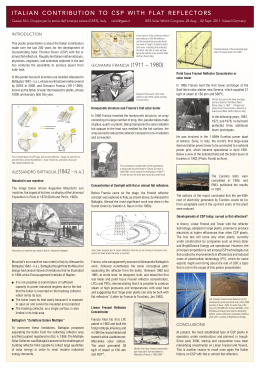
Figure 1-2 Overall view of the Portogruaro Civic Tower
Nevertheless, it appears adequate in this phase to verify the feasibility of the project on
a specific real case study. The Portogruaro Civic Tower was selected as a representative
case in this sense, in view of:
•
•
its architectural relevance;
the complexity and sensitivity of the problems related to an eventual restoring
intervention;
these aspects well justify an important investment in instruments, which will allow a
deep and timely control of the structural safety.
1.2 Scientific overview
1.2.1 The monitoring concept
With structural monitoring systems, reference is understood as the whole
instrumentation (hardware) and procedures (software), which aim at acquiring the time
evolution of certain measurements, which are supposed to be related to the safety
condition of a structure (usually strains, displacements, velocities, accelerations,
temperatures, forces).
In the field of civil engineering, bridges represent the most investigated typology of
structure in the past, and which deserves major interest for the present; with regards
specifically to Italy, historically relevant buildings and structures represent another
field where these applications have been recently developed. There are significant
differences in the manner of monitoring today with respect to two decades ago.
Monitoring has been seen in the past as an exceptional intervention, justified by the
importance of the structure (historical, economic or strategic relevance), or by the
immediate need to assess its uncertain safety condition. Today, the trend is to consider
4
Development of shared analysis instruments for the operation of a internet-based monitoring system
a monitoring system as a significant issue in the design of a new structure, or in the
retrofit of an existing one.
Many reasons explain such a change in philosophy: recent advances in sensors and
process methods (which allow lower installation and maintenance costs); the realization
by those entities, which are responsible for the maintenance of those structures, that it
is necessary to base a reliable assessment on well detailed and updated information;
some catastrophic failure (e.g.: the Silver Bridge in the 1967, the 3800 ft Bridge in
Seoul in the 1994; the Pavia Tower in Italy, etc.) contributed to advancements in this
direction.
1.2.2 Dynamic measurements
Data acquisition and interpretation criteria have also significantly changed. Early
investigation techniques focused on local measurements. Recently, research focused on
the possibility of obtaining more information on the safety condition of a structure on
the base of vibrational measurements. The basic idea behind this technology is that
modal parameters are a function of the physical properties of the structure; therefore,
changes in the physical properties will cause detectable changes in modal properties
(Doebling et al. 1998). The advantage of this approach is that a local measurement can
provide information, which is related with the global behaviour.
Early applications of dynamic monitoring in civil engineering date back to the
Seventies, and consisted of investigations aimed at the identification of the modal
properties of bridges subjected to ambient vibration (e.g. induced by traffic or wind) or
forced vibration (e.g. using a shaker) (Shepherd and Charleson 1971, Tanaka and
Davenport 1983, McLamore et al. 1971). A real improvement in the comprehension of
the actual relation between damage and dynamic behaviour of large-scale structures was
only possible with the availability of response data of the same structure both in the
undamaged and damaged conditions. The I-40 test (Farrar et al. 1994) represents the
first significant experience in this sense: the bridge was characterized in the undamaged
condition and in many situations of induced damage, and environmental conditions. The
installation of permanent data acquisition systems witnessed a strong increase in the
last decade (e.g. the Z-24 bridge, Maeck et al. 2000), to the point that today the design
of a monitoring system is becoming a part of the whole project of a new structure.
1.2.3 Monitoring of historical buildings
In the national ambit, relevant monitoring experiences focused mainly on the cases of
historical and monumental buildings. The monitoring of these structures deserves
special attention, not only for their relevance in Italy, but also for the special issues that
they involve:
•
•
•
the typological variety makes the generalization of outcomes of single experiences a
difficult task;
the behaviour of traditional materials (masonry, timber, etc.) is typically non-linear,
and exhibit high damping ratios;
the overall mechanical behaviour of a building is often not so evident, and hard to
model.
5
Chapter 1.Introduction
Moreover, the number of examples investigated in the past is still limited, both regards
to short-term vibrational tests (Vestroni et al. 1996) and to long term monitoring
(Bartoli et al. 1996). With respect to the latter aspect, a significant contribution was
also given by the Research Unit (RU) of Trento (Zanon 1999, Zanon 2000, Zanon et al.
2001, Zonta et al. 2002), as well as by the RU of Padova (Bosella et al. 1997, Modena
et al. 1999). In recent years, the interest is increasing in the application of these set-ups,
and this coincides with the rapid development of the techniques employed in the
operation of monitoring/control, particularly with reference to:
•
•
•
sensors (fibre optics, large scale sensors, etc.);
data evaluation techniques (advanced signal analysis, statistical pattern recognition,
data mining, etc.);
communication capabilities (internet, wireless technologies, remote control, etc.).
1.2.3.1 Sensors
With regards to fibre optic sensors, many applications both with Fiber Bragg Grating
and with Long Gauge Fiber Optic sensors are reported in the monitoring of bridges and
viaducts (Tennyson and Mufti 2000, Galante et al. 1999); however, experiences are
scarce in case of monumental buildings (Inaudi et al. 1997). In the same way, laser
sensors (such as non contact distantiometers, laser Doppler vibrometers...) which were
successfully utilized in mechanical engineering (Stanbridge and Ewins 1996), have still
yet to be extensively employed in civil engineering applications.
1.2.3.2 Data evaluation techniques
Another issue is the exploitation and elaboration of large amount of data provided by
monitoring operation. Advanced signal analysis techniques, such as time-frequency
analysis (Doebling et al. 1998), specifically apply to the elaboration of ambient
vibration acquisitions. An alternate way of processing time series is based on statistical
pattern recognition techniques (Soho et al. 2000). A more general approach to data
exploitation (which also applies to static series and to the information provided by
numerical modelling) utilizes well-established data-mining algorithms (Mitchell 1997,
Cherkassky and Mulier 1998), based on artificial intelligence concepts, such as neural
networks and decision trees.
1.2.3.3 Employment of information technologies
The dissemination of the Internet and of the information technologies in recent years is
deeply changing the philosophy of remote monitoring/control (Cherkassky and Mulier
1998, Rodellar et al. 1999). While usual procedures for data acquisition and elaboration
require long processing time, the Internet represents a potential tool for the execution of
these operations in real-time. Some significant experience in this sense are under
development in the United States, in the ambit of the NSF funded project NEES
(http://www.eng.nsf.gov/nees/) and at UCSD (http://monitoring.ucsd.edu, Elgamal et al.
2001, Fraser et al. 2002).
The objective of these networks is mainly a coordination effort among research groups,
consisting of:
•
6
sharing the specific experiences in the monitoring/safety assessment;
Development of shared analysis instruments for the operation of a internet-based monitoring system
•
defining general criteria and standards for the operation of possibly future
disseminated systems.
Until now, little attention has been given to the practical development of those on-line
instruments that will represent the core of the network, such as data acquisition tools,
signal processing tools, etc., and only few very limited examples are currently available
(http://webshaker.ucsd.edu). Indeed, the flexibility of the Internet would not require the
definition of rigid interchange standards, while these two aspects of the work can be
more fruitfully accomplished at the same time.
7
Chapter 1.Introduction
1.3 Objectives
The objective, which is intended to pursue with the development of this work, is that to
use the new data processing and Internet communication technologies, to create a
system of shared analysis instruments, which allows, as final purpose, to obtain a
structure safety index in real-time.
In this way it will be possible to check a structure in real time, simply using a web site,
without having to worry about the execution of all the analysis processes, that are
usually executed manually and that require a lot of time (months, or even years).
Besides, the versatility of this type of system is guaranteed by the fact that it is possible
to update or modify, in every moment, any of the link that compose the analysis chain.
The global functionality will remain unchanged on condition that the specifications for
the I/O data format are followed; obviously the final result will change, according with
the new analysis instruments.
1.3.1 Outlines of the thesis
The thesis aims are:
1. setting up the network server, with the creation of a master site, including: general
project information and basic tools for the development of the data exchange
network;
2. initial implementation of basic tools for the activation of a data interchange system
via the www;
3. state-of-the-art reports on data interchange protocols;
4. supply the starting kit of tools for the activation of a data interchange system via the
www.
5. describe a simple application of the webtools concepts
6. design for the installation of a monitoring system in the Portogruaro Civic Tower.
1.3.2 Aims of the investigation
This thesis has been developed in the sphere of a civil engineering research project,
whose objective is to define a rational and quantitative methodology for designing
improvement interventions of the safety level of historical and monumental structures,
exploiting in an optimal matter:
•
•
•
Information provided by monitoring systems;
Potentialities of active control systems;
Real-time processing and response capabilities of diffused networks.
Particularly, by the presentation of a theoretical case and the design for the installation
of a monitoring system in the Portogruaro Civic Tower, there is the intention of:
•
•
•
8
demonstrate the practical feasibility and the effectiveness of the real-time
monitoring via Internet philosophy;
create a sample monitoring system, that could be useful to the dissemination of that
philosophy;
give all the information necessary to join this research by the creation of new shared
analysis instruments.
Development of shared analysis instruments for the operation of a internet-based monitoring system
In this research project are involved the following Research Units (RU):
•
•
•
•
•
•
UniPI: Università degli studi di Pisa
UniGE: Università degli studi di Genova
PoliTO: Politecnico di Torino
UniTN: Università degli studi di Trento
UniPD: Università degli studi di Padova
UniPV: Università degli studi di Pavia
9
Chapter 1.Introduction
1.4 Method
In order to apply the concept of development of shared analysis instruments, in this
paragraph the webtools method has been brought in.
In substance a webtool is a CGI program, that receives data input, according to a fixed
standard, and send out other data (output), always according to the fixed standards. It is
not influenced by the data source, or by the their destination, and can be modify in
every moment, only respecting two bond:
•
•
the I/O communication standards;
the function that it has to execute.
The webtool, being a CGI program, can be executed only via an Internet call, using the
POST or the GET methods (which will be described later on); then that allows an
external user to use the analysis instruments without having to download and install on
his own personal computer any kind of program, applet, library, etc., disconnecting in
this way the program development from the operative system present on the final user
personal computer.
Therefore, in order to execute an automatic and real-time safety evaluation, a set of
webtools have to be linked in a “chain”, that allows to proceed from the data acquisition
executed directly on the structure to the generation of a safety index. This concept will
be diffusely stated during this thesis, through the presentation of two sample case
studies, in which the system to link in sequential way the webtools (in such a way as to
have an automatic data flow) will be presented.
An other interesting aspect of the webtools is that, besides being a totally automatic
procedure, it is possible to create a disseminated monitoring net through the generation
of a webtools chain. The term disseminated s connected to the fact that it is possible
that every webtool is physically residing in more than one server; therefore it is
possible that everyone, who intends to join to the working group, could keep his own
webtools on his server and make the via Internet utilization available for all the
remaining members of the working group, giving all the information useful to the use
(URL, I/O tables, etc.).
1.4.1 Webtools chain
The fact than a webtool needs exclusively data input in the standard format makes it
extremely versatile: in fact it is possible to use it “stand-alone” (giving directly the
requested input and receiving the output), otherwise to insert it in a webtools “chain”
(where the input is given to it directly from the webtools that precedes it in the chain,
and its output is received directly from the following webtool).
This chain is essentially made up of a “caller” program (that can be structured as a
webtool) that calls the webtools in the order necessary to execute the analysis, attending
to send the input data to the n-th webtool (in the appropriate format, requested from the
specifications of that webtool), to receive the output data and to send them as input to
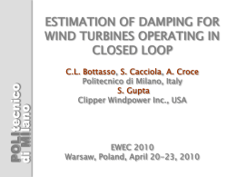
the (n+1)-th webtool. This operation scheme is shown in the following figure, referring
to the theoretical case study.
10
Development of shared analysis instruments for the operation of a internet-based monitoring system
Signal Generator
FFT
Peak Detector
Identification Tool
Structural Model
Safety Evaluation
Decision Making
Demonstrator.vi
Figure 1-3 Scheme of the Demonstrator.vi chain
The caller program can be in its turn a webtool residing in a server (that is a CGI and
therefore the execution request has to be sent to it through the Internet) otherwise a
program in execution on the client, that sends the CGI requests to the servers where the
webtools reside.
11
Chapter 1.Introduction
1.5 State-of-the-art
Some significant samples of new technologies applied to
this chapter. They are divided into three group: real-time
for the damage control and internet-based collaborative
has been the starting point for the development of the
thesis.
engineering
monitoring,
framework.
instruments
are introduced in
new technologies
This third group
presented in this
1.5.1 Real-time monitoring
The real-time monitoring system is certainly the most common use of new internetbased technologies in civil engineering. It has many advantages over post-processed
monitoring.
First, real-time monitoring provides a basis for rapid decision making under adverse
conditions. In order to be most effective, this response often needs to be initiated at the
height of the crisis. Real-time health and performance data can help to insure that
decisions are made with appropriate information. Indeed, many decisions might be
automated if real-time data is available.
A second more subtle motivation for real-time monitoring of structural health and
performance is that it can result in increased public awareness, understanding and
acceptance of monitoring technology. Public support and even public demand can be
extremely important factors in driving the development of refined systems and
improved technologies.(Wilfred D.Iwan “R-SHAPE: a real-time structural health and
performance evaluation”)
There are several samples of this monitoring technique actually working around the
Internet and here there is an overview.
A review of structural health monitoring literature 1996-2001 (Hoon Sohn, Charles R.
Farrar, Francois Hemez and Jerry Czarnecki)
Staff members at Los Alamos National Laboratory (LANL) produced a summary of the
structural health monitoring literature in 1995. This presentation will summarize the
outcome of an updated review covering the years 1996-2001. The updated review
follows the LANL statistical pattern recognition paradigm for SHM, which addresses
four topics:
1.
2.
3.
4.
operational evaluation
data acquisition and cleansing
feature extraction
statistical modelling for feature discrimination.
The literature has been reviewed based on how particular study addresses these four
topics. A significant observation from this review is that although there are many more
SHM studies being reported, the investigators, in general, have not yet fully embraced
the well-developed tools from statistical pattern recognition. As such, the
discrimination procedures employed are often lacking the appropriate rigor necessary
for this technology to evolve beyond demonstration problems carried out in laboratory
setting.
12
Development of shared analysis instruments for the operation of a internet-based monitoring system
The webshaker pilot project an internet framework for real-time monitoring and control
system of civil engineering structures (Micheal Fraser, Ahmed W. Elgamal and Daniele
Zonta)
A pilot project has been initiated with the goal of demonstrating the feasibility and
cost-effectiveness of a web-controlled, real-time monitoring and control system for
civil engineering structures. Emphasis is placed on the potential of the Internet for live
on-demand experimental-testing, sharing of information, and optimisation of resources,
both for research and practice purposes. The project is developing through a number of
actions, including the Webshaker Pilot Project, which consists of the demonstrative
installation of pilot web-controlled monitoring systems on some relevant buildings and
testing facilities.
The web address is: http://webshaker.ucsd.edu. At present, a small-scale pilot effort
consisting real-time dynamic tests. A digital video camera transmits live video, and the
structural response is made available using accelerometers. The user is allowed to run
dynamic tests, perform basic signal processing operations, and browse and download
from a database of archived data. The feasibility of this technology for both practical
and research applications is demonstrated.
The Webdome pilot project (Massimo Giuliani and Daniele Zonta)
This project has the aim to demonstrate that is possible to take advantage of the Internet
diffusion for the development of a real-time monitoring system prototype, which allows
the on-line and real time control of the structural response of a building.
In this project a network-based monitoring system has been developed. It is divided in
three sections: the instrumentation domain, the server side, and the client side. The
server-side section has the task to make available for the remote user the information
locally acquired by the instrumentation domain. Moreover the client-side section has
the task to make turn some simple programs on the Client computer instead of on the
server
The web address is: http://webdome.smartstructures.org. The web pages contain
information about the project, links to similar project, a live video from a digital
network camera fixed on the dome of the Mesiano Institute of Technlogy, a real-time
data-acquisition device and a set of analysis tools (FDD, FFT, WINDOW, POWER
SPECTRUM, MEAN VALUE REM, LINEAR TREND REM, etc.)
R-SHAPE: a real-time structural health and performance evaluation system. (Wilfred D.
Iwan)
This is a recent development in structural health and performance monitoring referred
to the Caltech Real-Time Structural Health and Performance Evaluation (R-SHAPE)
System. This system is installed in the Millikan Library Building on the campus of the
California Institute of Technology in Pasadena, California. It provides true real-time
health and performance monitoring tools.
The web address is: http://www.R-SHAPE.caltech.edu. The web page shows real-time
streaming data for acceleration, real-time Fourier Transform of acceleration and a live
image of the system itself
On-line structural health monitoring (Jyrki Kullaa)
Characteristics of on-line structural health monitoring were studied. On-line monitoring
works automatically and the damage-sensitive features must be predetermined although
no experience on damaged structure is available. Monitoring must be sensitive to detect
13
Chapter 1.Introduction
possible damage early for economic and safety reasons. On the other hand, the method
must be reliable without too frequent false indications of damage. An experimental
research of a health monitoring system was performed for a bridge model in the
laboratory. Two damage scenarios were introduced using additional point masses at
different locations of the bridge. It was found that using a high-dimensional feature
vector together with the principal component analysis both damage scenarios could be
clearly detected. The most reliable results were obtained using the first principal
component only. The natural frequencies and mode shapes were found to be the best
indicators of damage, whereas the damping ratios were relatively insensitive to the
introduced damage. The natural frequencies were also sensitive to environmental
variability causing false indications of damage.
1.5.2 New technologies for the damage control
Issues in wireless structural damage monitoring technologies (Jerome Peter Lynch,
Anne S. Kiremidjian, Kincho H. Law, Thomas Kenny and Ed Carryer)
A second-generation wireless sensing unit for real-time structural response
measurements has been designed and fabricated. Drawing upon advanced technological
developments in the areas of wireless communications, low-power microprocessors and
micro-electro mechanical system (MEMS) sensing transducers, the wireless sensing
unit represents a high-performance of structures. A sophisticated reduced instruction set
computer (RISC) microcontroller is placed at the core of the unit to accommodate onboard computations, measurement filtering and data interrogation algorithms. As a
result, the computational burden of the centralized data logger is placed on the
individual sensing units. A wide array of different sensors can be interfaced to the unit
delivering a sensor transparent module. The wireless infrastructure lowers overall
system installation costs by eliminating laborious cabling tasks. Initial validation of the
system is performed with the use of a small-scale two-story model structure
instrumented with our sensors and excited with a portable shaking table.
Telediagnosis and teleinspection potential of telematic techniques (K. Schilling)
The combination of modern information processing and telecommunication method
offers interesting application potential in the teleservicing of remote sites. This includes
operations and maintenance of plants as well as monitoring the state of construction
areas from remote centres. This paper presents as concrete example the teleoperations
of remote mobile robots in an outdoor environment. Details of the technical remote
control realisation on basis of the robot’s camera and range sensor data, transferred via
inexpensive Internet links are discussed. The application potential of these methods to
transfer remote sensor data and to perform control reactions for servicing tasks is
outlined.
1.5.3 Shared analysis instruments
Developing and distributing network based engineering solutions (M. Seifert, P. Parkhi,
V. Tandra Sistla, K.L. Lawrence)
The need to have easy access to the solutions of a variety of frequently occurring
engineering problems, has resulted in the development of a wealth of tools from
engineering handbooks to sophisticated desktop engineering software. In this paper, we
examine the use of internet/intranet-based methods for providing the tools that are
commonly needed by engineers in their daily work. Using the World Wide Web as the
14
Development of shared analysis instruments for the operation of a internet-based monitoring system
distribution medium and the Internet browser as the execution environment, Sun
Microsystem’s Java technology provides the foundation for the development of an
Engineer’s Tool Box (ETB) that provides a framework whereby independent
engineering software tools are linked, managed, and accessed globally via the Internet.
Individual applications are developed to address specific engineering problems using
simple, straightforward interfaces and are linked into the distributed ETB framework to
solve more complex problems. The capabilities and limitations of the Java platform for
developing and supporting such Internet based distributed engineering software tools
are discussed herein.
The need to have easy access to the solutions of common engineering problems
traditionally has been met with a wide range of reference handbooks, but more recently
sophisticated engineering software packages have been developed that allow complex
and diverse engineering problems to be efficiently modelled and solved.
A common database on structural assessment, monitoring and control (Bettina Geier,
Kent Mehr)
A common database on Structural Assessment, Monitoring and Control (SAMCO) shall
help to increase exchange of data and information within the SAMCO network
(www.samco.org). The network consists of engineers and researchers and they are both
contributors and end users. The database contains raw information, documentations,
reports, organizations, research projects, etc. within the field. For the realization of the
database web technology is used in combination with traditional database software. The
database is accessible via the Internet (http://www.samco.org/database and
http://samco.jrc.it). The data are available free of charge and shall supply the members
of the network with data.
Internet-enabled framework for collaborative development of non-linear dynamic
analysis program (J.Peng and Kincho H. Law)
It is well recognized that a significant gap exists in the state-of-the-art computing
methodologies and the state-of-practice in structural engineering analysis programs.
Most existing structural analysis programs lack the ability to allow continuous upgrade
to incorporate new developments. Advances in software engineering principles and
technologies may help alleviate some of these problems. Object-oriented methodologies
can provide software abstraction concepts, which encourage modularity and enhance
maintainability and extendibility of the code.
The Open System for Earthquake Engineering Simulation (OpenSees) is a PEER
sponsored project to develop a software framework for simulating the seismic response
of structural and geotechnical systems. OpenSees is intended to serve as the
computational platform for research in performance-based earthquake engineering at
PEER.
It is possible to retrieve more information about this project at the Internet site
http://eil.stanford.edu/law/ .
15
Chapter 1.Introduction
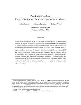
1.6 Networking
The basic tools, necessary for operating the interchange network of information for the
safety evaluation of civil engineering structures, have been developed and implemented.
Definition of the interchange protocols for:
• Data basing, of static and dynamic acquisition;
• Interchange of time series (e.g.: dynamic signal), in the web environment;
• Interchange of the FEM geometrical/mechanical information, control parameters and
outcomes of elaborations.
Figure 1-4 Layout of an Internet-based monitoring system
Reference will be made, as long as possible, to interchange standards compatible with
formats currently in use.
A start-up basic software package has been developed, to be utilized as a platform in
the development of the websites that will constitute the interchange network. This
package is available shareware (at the website mentioned before) for any
groups/researchers which intend to join the network, then.
The package will consist of:
•
•
•
16
a template of preformatted web-pages;
a template of elaboration program, based on the Common Gateway Interface (CGI)
protocol;
the on-line instruction for installation and operation.
Development of shared analysis instruments for the operation of a internet-based monitoring system
Moreover a master website has been developed, that will represent the main reference
point in the present Project and in the dissemination of the interchange network
philosophy. The site include:
•
•
a set of pages concerning the Project, including: general information on the Project;
the shared web-scripts; links to the other RU websites;
a set of pages concerning the interchange network, containing information,
examples, instruction, and software downloads.
17
Chapter 1.Introduction
1.7 Outlines
In this thesis all the information necessary to:
•
•
•
Create a webtool and make it available via internet;
Create a webtools chain, to realize a part, or the whole, of a real-time monitoring
structure of the safety state of a building;
Use the webtools developed by other components of the research group;
will be shown.
In order to do that, two case studies will be used, through the explanation of which all
the problems, with which it has to be dealt developing a system of this type, and the
way in which they have been solved, will be explained.
1.7.1 Common Gateway Interface concepts
In order to understand the operation of a webtools it is necessary to start from the
analysis of the communication system, on which they are based, that is the CGI. This
communication interface allows to a user (client) to request the execution of a program
(i.e. the webtool) placed on a remote server. The convenience of this type of interface is
that the client doesn’t have to install in its own personal computer any kind of software,
in that the program is executed totally remotely on the server. Once the program
execution has finished, the server will send to the client the requested information, in
the form of:
•
•
•
web pages, which are called “dynamic” (because their content changes according to
the data input coming from the client) in order to differentiate them from the
“static” ones, in which the content is fixed and can’t change according to the client
requests;
downloadable files for the client user;
data, in format coded according with the specifications, which the client will after
use as data input to send in the request to the following webtool (in the case in
which the client is making a chain of requests to webtools).
In this thesis the standard to follow for the format of the data which are transmitted
between webtool and webtool, and those which are transmitted between client and
server, will be shown.
1.7.2 Webtools development
Two case studies (Demonstrator and Portogruaro), on which the development of shared
analysis instruments for the operation of an Internet-based monitoring system has been
tested, will be presented. These cases are presented showing the functional scheme that
characterize them, explaining how the single data passing among the various webtools
happen, which of these data are considered acquired in a static way (that is a priori
fixed, not in real-time up-to-date) and which are instead considered acquired in
dynamic way (that is every time the analysis is executed, a procedure of data
acquisition, that supplies the new data in real time, is made active).
18
Development of shared analysis instruments for the operation of a internet-based monitoring system
An example of data considered acquired in a static way could be the FE model of the
structure, an example of data considered acquired in a dynamic way could be the signal
acquired from the sensors placed on the structure.
It is the case to notice how the data that are considered acquired in a static way, have
not to be thought fixed and not modifiable; really, it is enough to intervene in the
programming of the webtool, in order to modify also that type of data: but it is clear
that this kind of changing has nothing to do with the alterations happened on the
structure and that modify its safety level (a matter that there is in the case of variation
of the data acquired in a dynamic way).
1.7.2.1 Demonstrator
This case study refers to a single D.O.F. structure, as shown in Figure 1-1.
The problem in exam is totally ideal, but it could be thought as simplified scheme for
the analysis of a structure that has the greater part of the mass concentrated on the top
and that results solidly constrained at the base; a typical example of this type of
structural scheme is recognized in the pensile tanks.
Afterwards the functional scheme of this ideal case is reported.
Signal
Characteristics
Signal Generator
TH Signal
FFT Amplitude
Analysis
FD Signal
Peak Detector
Frequencies
Analytical Model
Identification
Tool
Mechanical
Features
Mass
Acceleration
Of Gravity (g)
Structural Model
Standards
Stress
Admissible stress
Safety
Evaluation
Geometrical
Features
Safety Index
Decision Making
Figure 1-5 Demonstrator flow-chart
The analysis aim is to determine the safety level in which the considered structure is,
starting from a Frequency Response Function generated in a casual manner and
19
Chapter 1.Introduction
proceeding to the structural identification (for which it is necessary to know the
analytical model and the geometrical and mechanical properties of the structure) and to
the structural model (for which it is necessary to know only the geometrical properties
of the structure).
The various passages of the flow-chart will be more diffusely explained stated in the
Chapter 2 and 3.
Respectively, in the Chapter 2 a conceptual explanation of the philosophy that guides
the development and the utilization of the webtools and in the Chapter 3 a technical
explanation of the communication system that uses the CGI, which is that based on the
webtools, will be supplied.
1.7.2.2 Portogruaro
Instead this case study refers to a real case of practical interest. In fact a system, which
allows the real-time monitoring of the Portogruaro Civic Tower, has been designed.
This system will allow to acquire in real time the value of the inclination angle and of
the temperature of some significant point of the structure; correlating these dynamic
data with the static ones obtained from:
•
•
•
tests of dynamic characterization, executed on the structure in the August 2002;
FE model analysis;
ULS analysis of the base section of the Tower.
It will be possible to obtain, in probabilistic term, a safety level of the structure in the
instant in which the program is executed.
The flow-chart of this system is reported in Figure 1-6.
The various passages of the flow-chart will be more diffusely exposed in the Chapters
4,5 and 6.
In the Chapter 4 a relation of the dynamic tests executed on the Tower, used for the
dynamic characterization of the structure, will be reported.
In the Chapter 5 the description of the FE model of the structure, used for the
evaluation of the stresses acting on the structure and of the load used for the analysis,
as well as the description of the analytical model used for the ULS analysis of the base
section, will be reported.
Finally in the Chapter 6 the design of a data acquisition system in real-time and the
correlation that is possible to establish between these dynamic data and those static
stated in the Chapters 4 and 5 will be reported.
20
Development of shared analysis instruments for the operation of a internet-based monitoring system
Data Acquisition
Survey
NDT tests
Network Camera
Transducer
TH Signal
Geometrical
Information
Constitutive Laws
Image
Temperature
Failure
Modeling
Image
Analysis
FFT Analysis
Tangent Behavior
FD Signal
Meshing
ABC
ABC
Data Processing
Inclination
Codes
Actions Model
Resistance Model
ABC
ABC
Data Processing
Parametric FEM
Actions
Evaluation
FRF
Modal Extraction
Modal Parameters
Trend
Actions
Identification
Mass Distribution
LS Assessment
Stability
Analysis
Structural Response
Max displacement
Mass
ABC
ABC
Safety Evaluation
Safety Index
Figure 1-6 Portogruaro safety evaluator flow-chart
21
2 Webtools
Abstract
What is a webtool and how does it work? In this section the technical information that
has to be known to be able to use a webtool or to connect two or more of them in a
chain that performs in an automatic way a series of analysis are given.
To understand the way of working of the system an example-case for studying has been
created (without any relationship with any real case) and here the chain of webtools is
shown to perform the analysis, together with the description of the webtools that
constitute it and of the kind of data that flow through it.
Sommario
Cos’è e come funziona un webtool? In questa sezione sono riportate le informazioni di
carattere tecnico da conoscere per poter utilizzare un webtool o per collegarne due o più
in una catena che esegue in modo automatico una serie di analisi.
Per comprendere il funzionamento del sistema è stato creato un caso studio di esempio
(senza attinenza con un caso realmente esistente) e qui viene presentata la catena di
webtools che è stata creata per eseguire l’analisi, insieme alla descrizione dei singoli
webtool che la compongono e del tipo di dati che fluiscono attraverso essa.
23
Chapter 2. Webtools
2.1 Introduction
In this Chapter all the information necessary to understand the philosophy that inspires
the webtools development has been stated; besides the information necessary for an
user to use all the webtools that have been developed during this thesis (and to create
some chains with the webtools already developed) has been supplied.
For all the technical information relative to the communication via Internet, that is
necessary to develop an own webtool and to share it with all the research group, it is
referred to the following Chapter 3, where the argument will be thoroughly stated.
2.1.1 What is a webtool?
A webtool is a CGI (Common Gateway Interface) program that needs a call via Internet
from a personal computer connected to the net to be executed.
It is physically residing in a personal computer connected to Internet (called server) and
then reachable from any personal computer that could be connected in its turn to
Internet (called client), using the webtool URL.
The following is an example of URL:
http://www.smartstructures.org/cgi-bin/remote_server/demontrator.vi
The personal computer, that send the request of execution of a CGI , is usually called
client; it is to notice that the same server, in the moment in which it sends a request to
another server (or also to itself) becomes a client. Therefore the server and client
concept is exclusively connected to the function that the personal computer is
accomplishing in that exact instant.
A webtool has to receive data input in order to be executed; these data must necessarily
respect the standard according with which the program has been implemented; it is
possible to provide that the program automatically assign some default values to the
variables, that haven’t been supplied as input; but if the data input don’t respect the
standard format, then the program execution will fail. For this matter it is important that
every webtool is accompanied with some documentation (preferably in the form of a
web page, in order to allow a better dissemination, otherwise in the form of .pdf
document) which specifies in a exact way the I/O standards and any default choice for
the variables to which the input value is not assigned (for the specification file, see the
Chapter 3).
24
Development of shared analysis instruments for the operation of a internet-based monitoring system
INPUT
OUTPUT
KEYS
VALUE
Key_1
Value_1
KEYS
VALUE
Key_1
Key_2
Value_1
Value_2
Key_2
…
Value_2
…
…
…
WEBTOOL
Figure 2-1 Communication scheme
The data, which are given in output by a webtool, change according to the way the
webtool has been implemented by the programmer; in fact it can produce:
•
•
•
web pages, which are called “dynamic” (because their content changes according to
the data input coming from the client) in order to differentiate them from the
“static” ones, in which the content is fixed and can’t change according to the client
requests;
downloadable files for the client user;
data, in format coded according with the specifications, which the client will after
use as data input to send in the request to the following webtool (in the case in
which the client is making a chain of requests to webtools).
According to the webtool be used stand-alone or linked in a chain with other webtools,
a type of output rather than the other will be chosen.
The TCP/IP is the data transmission protocol used in the transmission of CGI requests.
In fact, thanks to the utilization of a data transmission protocol so standard, it will be
possible to realize webtools in different programming languages (LabVIEW, PHP, Java,
MatLab, etc.) and operative systems, still maintaining the total compatibility.
Nevertheless this thesis will refer exclusively to webtools carried out with LabVIEW
and residing in a server with a Windows 2000 Professional Operative System.
2.1.2 What are the application of the webtool system?
A webtool is an instrument extremely versatile, because it can be used stand-alone, in
order to execute a simple analysis, otherwise connected in series with one or more other
webtools, in order to create a so called webtools chain (or webtools system).
For example, if the FFT_amplitude.vi webtool is token in consideration (which is one
of the webtools that compose the Demonstrator.vi chain), it receives as input a file
containing a signal and provides as output a file containing the signal Fast Fourier
Transform in amplitude. Evidently it can be used as a single instrument to execute the
Fast Fourier Transform of a signal; but, if I connect it in series after another webtool
which has as output data a file containing a signal (i.e. the signal_generator.vi ,
which is another of the webtools, that compose the Demonstrator.vi , that has as input
data the sampling length, the maximum amplitude of the signal and the signal frequency
25
Chapter 2. Webtools
of the sinusoidal signal), I will create a chain, where the data pass in an automatic way
from a webtool to another.
In this way it turns out clear that it is possible to use this important characteristic of the
webtool, in order to create complex systems, constituted by several webtools linked in
series among them, so that it is possible to execute complex analysis in an automatic
way an in real-time.
The advantage in comparison with the way of proceeding used until now in the
structural safety analysis is clear: before the data elaboration and carriage needed very
long times, now all that can happen in real-time, using the webtool system, and without
the need that the operators execute the data carriage from one instrument to another.
26
Development of shared analysis instruments for the operation of a internet-based monitoring system
2.2 Communication standards
2.2.1 Standards I/O
In this paragraph the communications standards, with which the webtools shown in this
thesis have been developed, have been described. It is absolutely necessary that they are
scrupulously followed, in order to can correctly use the webtools, that have been
implemented; and it is advisable that they are followed also for the development of new
webtools to share with the research group, in order to make maximum the compatibility
among instruments developed from different people.
2.2.1.1 Method
This environmental variable represents the method with which the CGI call to the
webtool is executed. It can assume several values (see Chapter 3), but those, that are
useful for the webtools aims, are:
•
•
GET method;
POST method.
All the webtools developed in this thesis use the POST method. It has been chosen to
use this method, because it doesn’t present length limits as regards the dimension of the
content sent through the request; instead the GET method presents a 1000 characters
limit: this represents a problem, because if you need to send abundance of data (i.e. a
file containing a signal) it is necessary to use communications protocols different from
those typical of the CGI (i.e. it is necessary to use the File Transfer Protocol to send the
file).
Therefore for the users that intend to develop their own webtools the use of the POST
method is advisable, so as to guarantee uniformity from the point of view of the
communication modality. This aspect is essential to guarantee the diffusion of this
system, in that it makes easier the webtools implementation, as regards the I/O part (in
fact, if the communication happens only with the POST method, it is not necessary to
insert into the program a procedure that controls the call method and that modifies the
input data consequently).
2.2.1.2 Encryption-type
The environmental variable Encryption-Type represents the type of encryption to
which the data are subjected before being sent to the webtool. In fact the system in
which the data are sent to the webtool provides that they are inserted in the
environmental variable content , using some field delimiters to separate the data, in the
case of more than one group of data are present (i.e. in the signal_generator.vi there
are three data groups: the length, the amplitude and the frequency).
This environmental variable can assume the following values:
•
•
•
application/x-www-form-urlencoded
multipart/form-data
text/plain
27
Chapter 2. Webtools
The encryption type used in all the webtools developed in this thesis is the
multipart/form-data , in that it is the only that allows the data sending of the file type
(that are necessary when it has to be sent a signal or a Fourier Transform).
This choice influences, as said, the form of the content and in the next paragraph this
aspect will be described in detail.
2.2.1.3 Content
The environmental variable content is the one that contains all the data sent from the
client to the server and that will be processed by the webtool, in order to provide the
output result (see Figure 2-1). Therefore it is essential that the content is defined in an
univocal way, so the program could deduce from it all the data necessary to the correct
operation.
As said in the previous paragraph, it has been chosen to use a multipart/form-data
encryption type. The delimiter, that is at the basis of this encryption type, is the one
that is called boundary and whose value is in the environmental variable
HTTP_CONTENT_TYPE (or Content-Type) ; in fact it is of the type:
HTTP_CONTENT_TYPE =
multipart/form-data; boundary=---------------------------7d37d20702e4
The value of the environmental variable Encryption-Type (as said, in this case it is
multipart/form-data ) and the one of the boundary are easily traceable in that string.
This boundary is the same for all the content and it is used to separate the different
data that are passed to the webtool through the CGI request.
The content has to assume a form of the following type (it is to notice that the bold
letters don’t appear in the content, but are used only to indicate the presence of special
characters, i.e. LF Linefeed, CR Carriage Return, HT Horizontal Tabulation, SP
Space):
[Boundary] LF CR
[Header_1 of Key_1] LF
[Other header] LF CR
CR
LF CR
[Value_1] LF CR
[Boundary] LF CR
[Header_1 of Key_2]
...
...
LF CR
LF CR
[Value_n] LF
[Boundary]--
CR
LF CR
where:
is the boundary , that you can retrieve in the
environmental variable Content-Type
[Header_1 of Key_n]
is the following string:
Content-Disposition: form-data; name=” [key_n] ”
[Other header]
are lines according to the RFC822 standard,
classifiable as general headers, entity headers and request headers (see
[Boundary]
28
Development of shared analysis instruments for the operation of a internet-based monitoring system
http://www.faqs.org/rfcs/rfc822.html Crocker D.H., “Standard for the
format of ARPA Internet text messages”)
[Value_n]
is the value of the Key_n variable.
Afterwards,
as
an
example, the
signal_generator.vi is reported:
content
given
as
input
to
-----------------------------7d32af2702e4 LF CR
Content-Disposition: SP form-data; SP name="Signal_period"
the
webtool
LF CR
LF CR
1 LF CR
-----------------------------7d32af2702e4 LF CR
Content-Disposition: SP form-data; SP name="Signal_amplitude"
LF CR
LF CR
1 LF CR
-----------------------------7d32af2702e4 LF CR
Content-Disposition: SP form-data; SP name="Signal_frequency"
LF CR
LF CR
10 LF CR
-----------------------------7d32af2702e4 LF CR
Content-Disposition: SP form-data; SP name="submit"
LF CR
LF CR
General LF CR
-----------------------------7d32af2702e4--
LF CR
The following elements of interest are recognizable:
•
•
“-----------------------------7d32af2702e4 ”: it is the boundary and, as it is
evident, it is used to separate the four data ( Signal_period , Signal_amplitude ,
Signal_frequency and submit ). It is to notice as the boundary that close the
content is the same of the one that separates the data, with the only difference that
the characters “ -- ” and the LF CR (Linefeed and Carriage Return) have been added
at the end of the string.
“ name="Signal_period" ”: it contains the name of the variable; the variable value
is contained in the following line (in this case the value of the Signal_period
variable is 1). It is to notice that between the line in which there is the variable name
and the line in which there is the value, a void line must be left.
In order to have an example of a webtool that receives as input also a data file, here the
content given as input to the webtool FFT_amplitude.vi is shown:
-----------------------------7d310923702e4 LF CR
Content-Disposition: SP form-data; SP
name="Signal_generator_file_content"; SP
filename="C:\Inetpub\wwwroot\cgibin\remote_server\Demonstrator\remote_signal_generator_file_output.txt"
LF CR
Content-Type:
SP text/plain LF CR
LF CR
29
Chapter 2. Webtools
0.000E+0 HT 2.000E-3
HT 1.200E-2 HT
HT 4.000E-3 HT 6.000E-3 HT 8.000E-3 HT 1.000E-2
…
…
9.860E-1 HT 9.880E-1
1 HT 9.980E-1 LF CR
0.000E+0 HT 1.253E-1
1 HT 6.845E-1 HT
HT 9.900E-1 HT 9.920E-1 HT 9.940E-1 HT 9.960EHT 2.487E-1 HT 3.681E-1 HT 4.818E-1 HT 5.878E-
…
…
19.511E-1 HT -9.048E-1 HT -8.443E-1 HT -7.705E-1 HT -6.845E-1 HT 5.878E-1 HT -4.818E-1 HT -3.681E-1 HT -2.487E-1 HT -1.253E-1 LF CR
LF CR
-----------------------------7d310923702e4 LF CR
Content-Disposition: SP form-data; SP name="t0" LF
CR
LF CR
0.000E+0 LF CR
-----------------------------7d310923702e4 LF CR
Content-Disposition: SP form-data; SP name="dt" LF
CR
LF CR
2.000E-3 LF CR
-----------------------------7d310923702e4--
LF CR
In this case, in addition to the elements shown in the previous case, there are the data
contained in the file, that represent the signal generated by the signal_generator.vi
webtool. This data are preceded by the usual boundary string and by the variable name;
in the first line after the boundary there is the filename . In the following line there is
the string “ Content-Type: “ followed by the type of data contained in the file (in the
cases of the Demonstrator.vi it is always referred to text file, so this parameter
assumes the “ text/plain ” value); then the text contained in the file starts after a LF
CR. After the file there are other variables necessary for the elaboration.
It has to be token care of all the not-displayable characters (those written in bold
characters), in that their absence yields the incorrect operation of the webtool, because
the decryption doesn’t work properly and the program can obtain the values of the input
data.
2.2.1.4 File Format
The data files, that are used by the webtools, must have a standard format, so as to
guarantee the compatibility among different webtools.
The following is the standard that has been fixed:
•
•
30
Every data series (an acquired channel, rather than a time history) must stay in the
same line of the file, that has to be closet by a LF CR
Every data in the series is separated from the following through a tabulation HT.
Development of shared analysis instruments for the operation of a internet-based monitoring system
In the demonstrator case study the input file for the FFT_amplitude.vi webtool
contains two series: in the first there is the time, in the second the amplitude.
2.2.2 How to make a webtool request
The execution of a CGI request can happen at two levels: the user one and the machine
one.
In the user level:
•
•
•
the webtool utilization has a graphic interface, where insert the variable values
(input data);
the output is given in a graphic interface (therefore the output variables values are
inserted in a web page);
it is not possible to build webtools chains that run in an automatic way, because the
I/O data passing between webtools can happen only in a manual way.
In the machine level:
•
•
•
the webtool utilization hasn’t a graphic interface and the input data are passed to the
webtool directly in the CGI request;
the output is not given in a graphic interface, but the output data are of the same
format of the input ones;
it is possible to build webtools chain that run in an automatic way, because the input
format is the same of the output one, so the output data of the n-th webtool can be
directly sent to the (n+1)-th webtool.
2.2.2.1 User level
The webtool is called directly from a web page, in which a form, where you can insert
all the values of the keys necessary for the webtool operation, must be present. Once
pressed the SUBMIT key in the HTML FORM, the CGI request are sent to the server
and elaborated.
The attributes of the HTML tag form must have the following values:
action
method
enctype
= required webtool URL
= sending request method (in this case, POST )
= encryption type (in this case, multipart/form-data )
The following HTML code is the complete FORM:
<form action="http://www.smartstructures.org/cgi-bin/webtool.vi"
method="post" enctype="multipart/form-data">
...
...
<input type="submit" value=”webtool”>
</form>
and in this case the parameters values are chosen by the user selecting them in the form
31
Chapter 2. Webtools
<select
<option
<option
<option
<option
name=”frequency">
value="1 khz">1 Khz</option>
value="2 khz">2 Khz</option>
value="3 khz">3 Khz</option>
value="4 khz">4 Khz</option></select>
or filling in the text box with numerical values
<input type="text" name="frequency">
or the text area
<textarea name="signal">
</textarea>
The name of the key variable is the one that is assumed by the attribute name of the
considered tag ( select , input , textarea , etc.); the value of the key variable is the
one that will be selected or inserted in the form by the user.
2.2.2.2 Machine level
In this level the CGI request is directly sent from a webtool to the following, using the
data transmission protocol TCP/IP; in fact through the use of a so standardized
transmission protocol it is possible to develop webtools in different programming
languages (LabVIEW, PHP, Java, MatLab, etc.), still maintaining the absolute
compatibility.
The request to send is a MIME (Multipurpose Internet Mail Extensions) message made
of a request line and of further optional data, as shown afterwards:
[Method] SP [cgi URL]
[Header_1] LF CR
[Header_2] LF CR
SP [Version] LF CR
…
…
[Header_n]
LF CR
LF CR
[Body]
LF CR
where:
the used method (the POST method will be always used in this
thesis)
[cgi URL] is the complete URI of the webtool to which the request is being
sent (it refers to a local resource of the asked server)
[Version] could be HTTP/1.0 or HTTP/1.1
[Header_n] are lines according to the RFC822 standard, classifiable as general
header, entity header and request header
(see http://www.faqs.org/rfcs/rfc822.html Crocker D.H., “Standard
for the format of ARPA Internet text messages”)
[Body]
is a MIME message.
[Method]
The needed headers are:
32
Development of shared analysis instruments for the operation of a internet-based monitoring system
•
•
SP multipart/form-data; SP boundary= [boundary]
Content-Length: SP [number of characters that composes the [Body] ]
Content-Type:
and the [Body] has the format described in the paragraph relative to the content .
Afterwards the request that is sent by the safety_evaluation.vi webtool to the
decision_making.vi webtool is reported as an example:
POST SP /cgi-bin/remote_server/Demonstrator/decision_making.vi SP
HTTP/1.0 LF CR
Content-length: SP 146 LF CR
Content-type: SP multipart/form-data; SP boundary=----------------------------7d3ab91708ba LF CR
LF CR
-----------------------------7d3ab91708ba LF CR
Content-Disposition: SP form-data; SP name="Gamma" LF CR
LF CR
1.807E+9 LF CR
-----------------------------7d3ab91708ba-- LF CR
2.2.2.3 Chain request methods
In the case it is intended to combine two or more webtools, so that they pass one to
another, in an automatic way, the input and output data, there are two conceptual
scheme to use: the serial one and the parallel one. In the following paragraphs are both
illustrated an the choice to use the parallel scheme is explained.
2.2.2.3.1 Serial request
Signal Generator
FFT
Peak Detector
Identification Tool
Structural Model
Safety Evaluation
Decision Making
Demonstrator.vi
Figure 2-2 Serial chain request
The operation according with this scheme is conceptually very simple: there is a master
webtool (the one denoted with Demonstrator.vi ), that is the one to which the first
request arrives (that could arrive from a web page, as well as from another webtools
chain) and that provides for activating the chain, sending the request to the first
webtool (in this case signal_generator.vi ); the output data of the first webtool pass
directly to the second as input data (then the first calls directly the second) and so on,
until the last one (in this case decision_making.vi ), that sends its output data to the
33
Chapter 2. Webtools
master webtool. Therefore the master webtool will provide for arranging the data in the
desired form for the final output (for example a web page).
2.2.2.3.2 Parallel request
Signal Generator
FFT
Peak Detector
Identification Tool
Structural Model
Safety Evaluation
Decision Making
Demonstrator.vi
Figure 2-3 Parallel chain request
Instead the operation of this second scheme is conceptually more complex: there is
always a master webtool, but in this case the caller is it; in fact the master webtool
calls, one at a time, in the desired order, the webtools that compound the chain,
arranging the output data of the n-th webtool in such a way as they could be sent as
input for the (n+1)-th webtool. Also in this case the master webtool will provide for the
arrangement of the data in the form desired for the final output.
In this thesis it has been chosen to use this type of scheme, because in the serial scheme
it is necessary to send along the chain all the data necessary to the webtools that
compose it, as well as the indications to reach all the webtools of the chain and in
which order: this requires the sending of big quantity of data from a webtool to
another, above all if the chain is very long and provides for the analysis if very
“voluminous”, considerably and uselessly slackening the entire process. Besides, if
something in the chain changes, it’ll result more practical to modify only the master
webtool, rather than all the data to send along the chain; this is useful in the case of a
webtool is not temporarily available: in fact it will be possible to substitute it with
another one that performs the same function, without having to change all the data flow.
2.2.3 Specification file
Every webtool, that is developed by a component of the research group, has to be
provided with a web page or a .pdf file to be found in Internet, in which the utilization
specifications have to be clearly shown; in fact they will be indispensable for a user that
intends to use a webtool developed by an another component of the research group.
Afterwards the point to follow in order to compile the specifications file are reported:
1. Short name: webtool name (it has to be univocal)
2. URL: webtool Internet address, to which the CGI request has to be sent
3. Scheme: I/O operation scheme
34
Development of shared analysis instruments for the operation of a internet-based monitoring system
4. Algorithm: explanation of the algorithm used by the webtool to execute the
requested operations
5. Input: it is a table containing the input variables names (“keys”), the variable
format, a default value (where presents), and possible restrictions on the variables,
in order to avoid execution stops or not meaningful results
6. Output: it is a table containing the output variables names (“keys”), their format
and a brief description of them
7. Document URL: Internet address of the documentation (possible web pages, .pdf
documents, etc.)
8. Graphic Interface: it contains the Internet address of the web pages where it is
possible to use the webtool with a user-friendly interface. If it is not available, the
variable is void
9. Comments: a brief description of the function accomplished by the webtool and
possible comments useful for the user
10. Contact info: information to contact the webtool developer (Surname, Name,
Organization, Telephone number, e-mail, etc.)
In the following Chapter 3 a specifications template file will be shown, while in this
paragraph an example, relative to the case of the signal_generator.vi webtool, is
presented.
Short name
URL
signal_generator
http://www.smartstructures.org/cgibin/remote_server/Demonstrator/signal_generator.vi
INPUT
Scheme
OUTPUT
KEYS
VALUE
Key_1
Value_1
Key_2
Value_2
…
…
Signal
Generator
KEYS
VALUE
Key_1
Value_1
Key_2
Value_2
…
…
If Sine Wave is represented by the sequence Y, the VI generates the
pattern according to the following formula:
y[i] = amp × sin(phase[i]), for i = 0, 1, 2, ..., n-1,
Algorithm
where amp = amplitude, n = number of samples (#s), and phase[i] is:
initial_phase + frequency × 360.0 × i/Fs
35
Chapter 2. Webtools
Key
period
amplitude
frequency
Input
Value format
Floating-point number in
scientific notation
Floating-point number in
scientific notation
Floating-point number in
scientific notation
Default
Restrictions
1
>0
10
>0
10
>0
Output
Key
signal
t0
dt
Document
URL
Comments
Value format
Description
Spreadsheet of HT (Horizontal
The file containing the generated signal
Tabulation) separated values
Floating-point number in
Initial time of the Time history
scientific notation
Floating-point number in
1/Sampling ratio
scientific notation
http://www.smartstructures.org/cgibin/remote_server/Demonstrator/signal_generator.vi
This function generates a sinusoidal signal, knowing the period, the
amplitude and the frequency of the curve
Graphic
Interface
-
Contact info
All. Ing. Stefano Toffaletti,
Dipartimento di Ingegneria Meccanica Strutturale,
Università degli Studi di Trento,
e-mail: [email protected]
36
Development of shared analysis instruments for the operation of a internet-based monitoring system
2.3 VI starting kit
G programming, inside the Internet Toolkit add-ons package for LabVIEW, has been
chosen to create Common Gateway Interface (CGI) scripts that perform server
operations, that is the webtools.
The choice to use LabVIEW as programming language has been justified by the fact
that it is a software provided with a lot of included functions for the data acquisition
and their analysis, as well as with a rich library containing the .dlls for the operation of
the acquisition cards. Nevertheless it has been necessary to modify the included
function for the CGI utilization ( URL GET http Document.vi ), in that it is based on
the GET method for the request sending (and the webtools developed during this thesis
are based on the POST method for the request sending, as explained in the beginning of
this Chapter).
A set of web pages, where it is possible to download all the webtools that compose the
chains of the two considered case studies ( Demonstrator.vi and Portogruaro.vi ),
are available in the Internet site developed during this thesis. For the description of
these webtools, see Chapter 3 ( Demonstrator.vi ) and 6 ( Portogruaro.vi ).
Moreover, some subVI, written in LabVIEW programming language, useful for the
management of the CGI communications among webtools have been made available in
the same web pages, in such a way as everyone will be able to create his own chain
system.
The operation of this webtools is briefly described afterwards.
37
Chapter 2. Webtools
2.3.1 URL POST HTTP Document.vi
This subVI is marked by the following icon:
It retrieves a document specified by http URL and stores it in a specified file or returns
the contents as a string. The URL must refer to an HTTP document and can be in full or
partial format. The URL can include a user name and password for authentication. The
method used is POST.
A part of the diagram is shown in the following picture.
Figure 2-4 The URL Post HTTP Document.vi diagram
2.3.1.1 I/O
The I/O parameters for this subVI are the following:
38
Development of shared analysis instruments for the operation of a internet-based monitoring system
content-type in
http URL
file path
url-encoded content in
follow redirects
error in
content-length
full document URL
file path out
success
error out
content out
Input table
It is the MIME type of the request content
The location of the document
It specifies where to save the document. The default value is
<Not a path> , indicating that document should be returned in
content
It is the content of the request, encoded as shown in 2.2.1.3
It indicates whether the VI follows HTTP redirection replies.
The default is TRUE or follow redirects
It describes error conditions occurring before the VI executes.
If an error has already occurred, the VI returns the value of the
error in cluster in error out
It is the length of the url-encoded content in
It
It
It
It
It
Output table
is the full URL from which the document was retrieved
is the path to the file where the document was saved
indicates whether the document was retrieved successfully
describes error conditions occurring during the VI execution
contains the content of the retrieved document if file path is
<Not A Path>
content-type out
It is the MIME type of the retrieved document
39
Chapter 2. Webtools
2.3.2 Content analysis.vi
This subVI is marked by the following icon:
It receives as input the content encoded according to the encryption type
multipart/form-data and generates an array containing the keys and the values,
according to the conceptual scheme of the specifications file.
A part of the diagram is shown in the following picture.
Figure 2-5 The Content analysis.vi diagram
2.3.2.1 I/O
The I/O parameters for this subVI are the following:
cgi connection info
env
content
40
Input table
It is s a cluster containing information identifying this CGI
request
It is s the environmental variables parameter
It is a string containing the content of the request
Development of shared analysis instruments for the operation of a internet-based monitoring system
content-type
boundary
keyed array
Output table
It is the MIME type of the request content
It is boundary parameter value, retrieved from the content-type
environmental variable
It is an array containing in the first column the type of data
(F=File or D=single Data), in the second the key and in the
third the value
2.3.3 Content encoder.vi
This subVI is marked by the following icon:
It receives as input the content in the cluster format and send as output the content in
the MIME format specified in the content-type in variable.
A part of the diagram is shown in the following picture.
Figure 2-6 The Content encoder.vi diagram
41
Chapter 2. Webtools
2.3.3.1 I/O
The I/O parameters for this subVI are the following:
content-type in
content cluster
file description cluster
boundary
content out
42
Input table
It is the MIME type of the request content
It is a cluster containing two fields: key and value
It is a cluster containing three fields: key, type and filename.
Type is the type of data (F=File or D=single Data)
It is boundary parameter value, retrieved from the content-type
environmental variable
Output table
It is the MIME type of the request content
Development of shared analysis instruments for the operation of a internet-based monitoring system
2.3.4 File analyzer.vi
This subVI is marked by the following icon:
In the case in which there are some data in the file format in the CGI request content,
this subVI extracts the file content (in string format) and its name (in string and in path
format).
A part of the diagram is shown in the following picture.
Figure 2-7 The File analyzer.vi diagram
2.3.4.1 I/O
The I/O parameters for this subVI are the following:
43
Chapter 2. Webtools
cgi env
file name (if remote)
type of request
boundary string
Input table
It is s a cluster containing information identifying this CGI
request
It is s the environmental variables parameter
It is a string containing the content of the request
It is the type of the request
It is the boundary string
file uploaded name
file uploaded content
file uploaded name
Output table
It is the name of the file, with the complete path
It is the content of the file
It is the name of the file
cgi content
44
Development of shared analysis instruments for the operation of a internet-based monitoring system
2.3.5 Find boundary.vi
This subVI is marked by the following icon:
Knowing the environment variable, this subVI sends in output the value of the contenttype variable and of the boundary variable.
A part of the diagram is shown in the following picture.
Figure 2-8 The find boundary.vi diagram
2.3.5.1 I/O
The I/O parameters for this subVI are the following:
env
Input table
It is s the environmental variables parameter
45
Chapter 2. Webtools
content-type
boundary
Found
Output table
It is the MIME type of the request content
It is boundary parameter value, retrieved from the content-type
environmental variable
It is a boolean variable; it is TRUE if the boundary has been
found
2.3.6 Ptolemy to graph.vi
This subVI is marked by the following icon:
It generates the HTML code to use the Ptolemy.plot applet; this applet is used to
display the content of a data file in a graph.
A part of the diagram is shown in the following picture.
Figure 2-9 The ptolemy to graph.vi diagram
46
Development of shared analysis instruments for the operation of a internet-based monitoring system
2.3.6.1 I/O
The I/O parameters for this subVI are the following:
Input table
server IP
It is the IP address of the server where there is the applet
ptolemy archive path
It is the path of the file “Ptolemy.plotapplet.jar”
ptolemy_output
file It is the path of the file containing the HTML code generated
path
HTML code out
Output table
It is a string containing the HTML code generated
47
Chapter 2. Webtools
2.4 Demonstrator.vi
2.4.1 Formalism used in the flow-chart
In the flow-charts shown in this thesis it is referred to the following formalism:
Webtool
Data
ABC
ABC
Database
It represents the execution of a tool (it can be a webtool
in the case of the tried data are of dynamic type, or an
analysis instrument of the classical type, if the tried data
are of static type).
It represents the data that are sent from a tool to the
following one.
It represents a database, that is a point in which a set of
data is stored up.
It represents the flow of data of dynamic type from a
webtool to the following one through the Internet. The
dynamic data are data that are up-to-date every time the
webtools chain is executed.
It represents the flow of data of static type from a
webtool to the following one. The static data are data that
are not up-to-date every time the webtools chain is
executed; nevertheless, they can be modified without
having to program again the webtools, being they
provided as input data for the webtool.
It represents the flow of data of embedded type. This type
of data are fixed inside the webtool and they can’t be
modified, but programming them again.
2.4.2 Problem statement
In order to make clear the operating principle of the development of shared analysis
instruments, a set of sample analysis instruments applied on a ideal case study have
been made. This study case is represented by a simple 1-DOF structure, constituted by a
rod embedded at the base, with all the mass concentred on the other end, as shown in
the figure (this is the simplified representation of a pensile tank).
48
Development of shared analysis instruments for the operation of a internet-based monitoring system
E,J,L
m
Figure 2-10 Structure schematization of the Demonstrator case study
Figure 2-11 An example structure of a pensile tank
Therefore the problem that is dealt with is that of the safety evaluation of such
structure, stressed in arbitrary manner. The analysis simulates the presence of an
accelerometer placed in the mass barycentre, that allows the recording of a Time
History signal.
This signal is subjected to the Fast Fourier Transform in amplitude analysis, deducing a
Frequency Domain signal. The FD Signal is sent to the peak detector, that characterizes
49
Chapter 2. Webtools
the peaks of this function: the biggest of these correspond to the natural frequency of
the structure.
The natural frequency so obtained is sent to the vibrational model of the structure,
through that it is possible to identify the mass value of the system.
The system mass, multiplied by the gravity acceleration value and divided by the base
area of the rod, gives the stress value in the base section.
Comparing this value with the admissible one, get from the standards, a safety index is
obtained, that, compared with limit values, allows to evaluate the safety level of the
structure.
The flow-chart of such system is shown afterwards:
Signal
Characteristics
Signal Generator
TH Signal
FFT Amplitude
Analysis
FD Signal
Peaks number
Peak Detector
Frequencies
Vibrational Model
Identification
Tool
Mechanical
Features
Mass
Acceleration
Of Gravity (g)
Structural Model
Standards
Stress
Admissible stress
Safety
Evaluation
Geometrical
Features
Safety Index
Decision Making
Figure 2-12 Demonstrator.vi flow-chart
In the following paragraph the data format and the operation of the webtools will be
briefly shown. As regards the usage specifications, see the following Chapter.
50
Development of shared analysis instruments for the operation of a internet-based monitoring system
2.4.3 Description of the data flow
In this paragraph every webtool has been analysed, giving prominence to the input data,
the output ones and the embedded ones.
Signal Generator:
The analysis simulates the presence of an accelerometer placed in the mass barycentre
of the structure (as shown in Figure 2-13), that allows the recording of a Time History
signal.
Figure 2-13 Position of the accelerometer
.
INPUT
KEYS
VALUE FORMAT
Length
Floating-point number in scientific
notation
Amplitude
Floating-point number in scientific
notation
Frequency
Floating-point number in scientific
notation
Sinusoidal signal
Signal
Characteristics
Signal Generator
Amplitude (mm)
1.5
1
0.5
0
-0.5
-1
-1.5
TH Signal
0
1
2
3
4
5
6
7
8
9
10
Time (s)
OUTPUT
KEYS
VALUE FORMAT
Signal
Spreadsheet of HT (Horizontal
Tabulation) separated values
t0
Floating-point number in scientific
notation
dt
Floating-point number in scientific
notation
Figure 2-14 signal_generator.vi flow-chart
51
Chapter 2. Webtools
FFT Amplitude Analysis:
Therefore the Fast Fourier Transform in amplitude analysis has been executed on that
signal.
INPUT
KEYS
VALUE FORMAT
Signal
Spreadsheet of HT (Horizontal
Tabulation) separated values
t0
Floating-point number in scientific
notation
dt
Floating-point number in scientific
notation
FFT Amplitude
FFT Amplitude
Analysis
Amplitude
TH Signal
FD Signal
0.8
0.7
0.6
0.5
0.4
0.3
0.2
0.1
0
-0.1
0
5
10
15
20
25
freque ncy (Hz)
OUTPUT
KEYS
VALUE FORMAT
Signal_amplitude
Spreadsheet of HT (Horizontal
Tabulation) separated values
t0
Floating-point number in scientific
notation
dt
Floating-point number in scientific
notation
Figure 2-15 FFT_amplitude.vi flow-chart
Peak detector:
The result is a function (frequency, amplitude), the maximum value pf which represents
the natural frequency of the structure.
INPUT
KEYS
VALUE FORMAT
Signal_amplitude
Spreadsheet of HT (Horizontal Tabulation)
separated values
t0
Floating-point number in scientific notation
dt
Floating-point number in scientific notation
Peaks_number
Floating-point number in scientific notation
FFT Amplitude
Peaks number
Peak Detector
Amplitude
FD Signal
Frequencies
0.8
0.7
0.6
0.5
0.4
0.3
0.2
0.1
0
-0.1
0
5
10
15
20
freque ncy (Hz)
OUTPUT
KEYS
VALUE FORMAT
Peaks_value
Spreadsheet of HT (Horizontal
Tabulation) separated values
Peaks_number
Floating-point number in scientific
notation
Figure 2-16 peak_detector.vi flow-chart
52
25
Development of shared analysis instruments for the operation of a internet-based monitoring system
INPUT
Identification tool:
Once determined the natural frequency of the system, it is applied to the vibrational
formulation of the 1 DOF system, in order to obtain the mass value of the structure. In
this part of the analysis also the embedded data (E,J,L) come into play.
KEYS
VALUE FORMAT
Peaks_value
Spreadsheet of HT (Horizontal
Tabulation) separated values
Peaks_number
Floating-point number in scientific
notation
Frequencies
Vibrational Model
Frequencies
f =
Identification
Tool
Mechanical
Features
Mass
Geometrical
Features
1
3⋅ E ⋅ J
⋅ 3
l ⋅M
2 ⋅π
OUTPUT
M=
KEYS
VALUE FORMAT
Mass
3⋅ E ⋅ J
l 3 ⋅ ( 2 ⋅π ⋅ f )
2
Floating-point number in scientific
notation
Mass
Figure 2-17 identification_tool.vi flow-chart
INPUT
Structural Model:
Therefore, inserting the mass into the structural model shown in Figure 2-18, it is
possible to determine the value of the compression stress at the base of the pillar,
schematised as a empty cylinder.
Also in this case there are some embedded data (g and A).
KEYS
Mass
VALUE FORMAT
s
Floating-point number in scientific
notation
Mass
Acceleration
Of Gravity (g)
Structural Model
D
Geometrical
Features
OUTPUT
Stress
KEYS
Sigma
Mass
VALUE FORMAT
Floating-point number in scientific
notation
σ=
M ⋅g
A
Mass
Figure 2-18 structural_model.vi flow-chart
53
Chapter 2. Webtools
INPUT
Safety Evaluation:
The compression stress so evaluated has been related to the admissible one, deduced
from the standards (embedded data), obtaining a Safety Index.
KEYS
VALUE FORMAT
Sigma
Floating-point number in scientific
notation
Stress
Stress
Standards
Safety
Evaluation
Admissible stress
γ=
σ
σ
OUTPUT
Safety Index
KEYS
Gamma
VALUE FORMAT
Safety Index
Floating-point number in scientific
notation
Figure 2-19 safety_evaluation.vi flow-chart
INPUT
Decision Making:
Comparing this Safety Index with some limit values it is possible to supply a real time
assessment of the safety state of the structure.
KEYS
Gamma
VALUE FORMAT
Floating-point number in scientific
notation
Safety Index
OUTPUT
Decision Making
KEYS
Decision
VALUE FORMAT
String
Figure 2-20 decision_making.vi flow-chart
54
3 Common Gateway Interface
concepts
Abstract
This chapter is addressed to who intends to develop some new webtools and share them
for the utilization via Internet from other people. Therefore it contains information on
(1) the systems of communication via Internet based on the CGI protocol, (2) the
installation of a server that allows the execution of CGI requests and (3) the installation
of a web server, for the visualization of the web pages related to the webtool. Lastly the
content that has to have the specifications file is shown; this file has necessarily to
accompany every webtool.
Sommario
Questo capitolo è dedicato a chi intenda sviluppare dei nuovi webtools e condividerli
per l’utilizzo via Internet da parte di altre persone. Quindi contiene le informazioni sui
sistemi di comunicazione via Internet basati sul protocollo CGI, sull’installazione di un
server che permetta l’esecuzioni di richieste CGI e sull’installazione di un server per
pagine web. Infine viene presentato il contenuto che deve avere il file di specifiche, che
deve necessariamente accompagnare ogni webtool.
55
Chapter 3. Common Gateway Interface concepts
3.1 Introduction
While the previous Charter has been addressed mainly to who intends to use some
webtools developed by someone else, this Chapter has been devoted to who intends to
develop his own webtools, to make available to anyone intends to use them via Internet.
Therefore in this Chapter information on the following topic will be supplied:
•
•
•
•
of technical character on the data transmission, using the CGI;
on the installation of a web server on the own personal computer;
on the installation of a CGI server on the own personal computer;
on the content of the specifications file, that has to be enclosed to the developed
webtool (it will be included also a template of the specification file).
3.1.1 Static and dynamic data
The data exchange through Internet can happen substantially following two
fundamentally different methodologies:
•
•
static data exchange;
dynamic data exchange;
The data exchange in static way is commonly the one that happens when you enter,
using a web browser, in a web page containing text, images, downloadable file and all
the other things that can exist in a electronic format; but the user can’t interact in a
“personal” way with the information that has made available.
Instead a dynamic content is something (text, images, etc.) that is sent to the browser
from the user in a “personal” way on the base of his requests. An immediate example of
this kind of content is any mail server (e.g. hotmail), that, according to the user
connected to the site, sends to the browser the personal content of the user (in this case
the received e-mail). Nowadays there are more and more cases of internet sites that
provide pages with dynamic content of various kind; the thing of more interest for this
thesis is base concept of the dynamic page utilization.
In fact the request, that is sent to the web server for a dynamic page, is substantially
different from the one that is sent for a static page. In fact this last one has its own URL
address, that is sufficient to insert into the browser to retrieve it, using exclusively the
HTTP protocol.
Instead the request for a dynamic type of content needs the use of a CGI program, that
“reads” the request, “creates” the page with the requested features and “sends” it to the
client browser; therefore the page, so requested, doesn’t have an own URL address, but
is created by the server at the moment of the request from the client.
56
Development of shared analysis instruments for the operation of a internet-based monitoring system
3.1.2 Terminology and abbreviations
Here there is the meaning of the terms used in this chapter.
•
•
•
•
Client: is a process (program) that sends a message to a server process (program),
requesting that the server perform a task (service). Client programs usually manage
the user-interface portion of the application, validate data entered by the user,
dispatch requests to server programs, and sometimes execute business logic. The
client-based process is the front- end of the application that the user sees and
interacts with. The client process contains solution-specific logic and provides the
interface between the user and the rest of the application system. The client process
also manages the local resources that the user interacts with such as the monitor,
keyboard, workstation CPU and peripherals. One of the key elements of a client
workstation is the graphical user interface (GUI). Normally a part of operating
system i.e. the window manager detects user actions, manages the windows on the
display and displays the data in the windows.
Server: a server process (program) fulfils the client request by performing the task
requested. Server programs generally receive requests from client programs, execute
database retrieval and updates, manage data integrity and dispatch responses to
client requests. Sometimes server programs execute common or complex business
logic. The server-based process "may" run on another machine on the network. This
server could be the host operating system or network file server; the server is then
provided both file system services and application services. Or in some cases,
another desktop machine provides the application services. The server process acts
as a software engine that manages shared resources such as databases, printers,
communication links, or high powered-processors. The server process performs the
back-end tasks that are common to similar applications.
User agent: is a particular kind of client, that starts an HTTP request (typically it is
the browser).
Origin server: the server that physically have the requested resource (it is the last
one of a chain).
Here there is the meaning of some abbreviations used in this chapter:
•
•
•
•
•
•
•
•
CGI: Common Gateway Interface is a standard for communication between Web
documents and CGI scripts you write
DNS: Domain Name Server is a distributed Internet directory service. It is used
mostly to translate between domain names and IP addresses, and to control Internet
email delivery
FTP: File Transfer Protocol
HTTP: Hyper Text Transfer Protocol
I/O: Input / Output communications
MIME: Multi-purpose Internet Mail Extensions. It extends the format of Internet
mail to allow non-US-ASCII textual messages, non-textual messages, multipart
messages bodies, and non-US-ASCII information in message headers
TCP: Transfer Control Protocol
URI: Uniform Resource Identifier is the generic set of all names/addresses that are
short strings that refer to resources
57
Chapter 3. Common Gateway Interface concepts
•
•
58
URL: Uniform Resource Locator is an informal term associated with popular URI
schemes: http, ftp, mailto, etc.
WWW: World Wide Web
Development of shared analysis instruments for the operation of a internet-based monitoring system
3.1.3 Overview
The Common Gateway Interface (CGI) is a standard for interfacing external
applications with information servers, such as HTTP or Web servers. A plain HTML
document that the Web daemon retrieves is static, which means it exists in a constant
state: a text file that doesn't change. A CGI program, on the other hand, is executed in
real-time, so that it can output dynamic information.
The CGI programs need to reside in a special directory, so that the Web server knows to
execute the program rather than just display it to the browser; this directory is /cgibin , in the cgi-server root directory (it could be different from the Web-server one, if
there are two or more servers active on the same computer).
This directory is usually under direct control of the webmaster, prohibiting the average
user from creating CGI programs, for security questions.
A CGI program can be written in any language that allows it to be executed on the
system, such as:
•
•
•
•
•
•
•
•
LabVIEW
C/C++
Fortran
PERL
TCL
Any Unix shell
Visual Basic
AppleScript
It just depends on what you have available on your system.
59
Chapter 3. Common Gateway Interface concepts
3.2 Client-server communications
When you click on a link container in a web page, the browser starts to change
information with the server pointed from that link.
When you insert an URL in the field “location” of the browser, or when you click on a
link in a web page, it is pointing to a certain web page contained in a computer (a
server). A web server is a process that runs continually on a machine, waiting for
requests to satisfy. When the server receives a request, it try to satisfy it. That is, when
you click on a link, the browser makes the request of a web page, the server receives
the request and search that page; when it finds the page, sends it to the web browser.
The language that server and client use in order to exchange information is the HTTP.
If a URL is analysed, you will find four parts:
http://webtools.smartstructures.org/webtools/index.asp
http
webtools.smartstructures.org
webtools
index.asp
•
•
•
•
method name (or service)
server name (or IP address)
optional path
web page name
the method name could be HTTP, FTP, NEWS (newsgroups), MAILTO (SMTP, i.e.
email), etc.
the server name denotes the name of the computer where the web page resides.
the URI (i.e. the path) with the name of the requested file (relative to the home
directory of the server)
the web page name, that is the name of the file.
When you click on the link, the client (the web browser) activates a connection between
the computer client and the server webtools.smartstructures.org, requiring a web page
with the file name “index.asp”. At this point the server receives the request and
searches the page. If the server finds it, sends it to the client, otherwise sends the
following error message: “404 not found”, Lastly the server close the connection.
Until the version 1.0 the HTTP was a “stateless” protocol, that means that every request
made from the client to the server requires the establishment of a new connection
(unlike other protocol as FTP or Telnet, where the client establishes an only connection
and can make several requests during this connection); that is every object contained in
the web page requires a new connection. During a new request, the server is not able to
know anything about the previously made request.
The new protocol HTTP 1.1 (HTTP-NG or HTTP Next Generation) allows a connection
for more than one request; so, for example, it is possible to read a whole web page
establishing only one connection; in this way the page will be downloaded faster.
Then the web server is only a program that run continuously waiting for some requests.
When a request is satisfied and the connection is closed, the server is again ready for
new requests. The client, through the browser, can require HTML documents, images,
sounds, videos, scripts, etc.
However, a script doesn’t be received, but it is executed by the server, sending to the
client the result of this execution.
A script is a program that acts as an interface between a client, a web server, the
operative system, the hardware peripherals or also other servers.
60
Development of shared analysis instruments for the operation of a internet-based monitoring system
The programming languages used for the script writing can be of different type,
according to the operative system used by the server and to the type of program the is
used as web server. The common thing between the different languages is the standard
of I/O communication, that allows the total interaction between server that supports
different languages. In fact it is possible to write two or more script in different
programming languages, but that receive the same input and send the same output.
In this thesis, two server have been used:
•
•
the IIS server, used for the requests of HTML pages, containing information and
links for the download;
the LabVIEW server, used to execute the script required by the client; these scripts
execute locally in the server the required operations, and send the required output
(e.g. HTML pages, spreadsheet data file, images, etc.)
Further in the Chapter it will be shown how to install and to configure both the servers;
however it is to notice that this is only one of the possible choice that can be done; that
because in the use of script CGI the only thing, that the programmer is interested in, is
the standard I/O; while there is no interest in their programming languages.
3.2.1 Request method definitions
This paragraph has been taken from the “FRC 2068: Hypertext Transfer Protocol –
HTTP/1.1” of the Network Working Group (January 1997).
The set of common methods for HTTP/1.1 is defined below. Although this set can be
expanded, additional methods cannot be assumed to share the same semantics for
separately extended clients and servers.
The Host request-header field must accompany all HTTP/1.1 requests.
3.2.1.1 Safe and Idempotent Methods
3.2.1.1.1 Safe Methods
Implementers should be aware that the software represents the user in their interactions
over the Internet, and should be careful to allow the user to be aware of any actions
they may take which may have an unexpected significance to themselves or others.
In particular, the convention has been established that the GET and HEAD methods
should never have the significance of taking an action other than retrieval. These
methods should be considered "safe." This allows user agents to represent other
methods, such as POST, PUT and DELETE, in a special way, so that the user is made
aware of the fact that a possibly unsafe action is being requested.
Naturally, it is not possible to ensure that the server does not generate side-effects as a
result of performing a GET request; in fact, some dynamic resources consider that a
feature. The important distinction here is that the user did not request the side-effects,
so therefore cannot be held accountable for them.
3.2.1.1.2 Idempotent Methods
61
Chapter 3. Common Gateway Interface concepts
Methods may also have the property of "idempotence" in that (aside from error or
expiration issues) the side-effects of N > 0 identical requests is the same as for a single
request. The methods GET, HEAD, PUT and DELETE share this property.
3.2.1.2 OPTIONS method
The OPTIONS method represents a request for information about the communication
options available on the request/response chain identified by the Request-URI. This
method allows the client to determine the options and/or requirements associated with a
resource, or the capabilities of a server, without implying a resource action or initiating
a resource retrieval.
Unless the server's response is an error, the response must not include entity
information other than what can be considered as communication options (e.g., Allow is
appropriate, but Content-Type is not). Responses to this method are not cacheable.
If the Request-URI is an asterisk ("*"), the OPTIONS request is intended to apply to the
server as a whole. A 200 response should include any header fields which indicate
optional features implemented by the server (e.g., Public), including any extensions not
defined by this specification, in addition to any applicable general or response-header
fields. An "OPTIONS *" request can be applied through a proxy by specifying the
destination server in the Request-URI without any path information.
If the Request-URI is not an asterisk, the OPTIONS request applies only to the options
that are available when communicating with that resource. A 200 response should
include any header fields which indicate optional features implemented by the server
and applicable to that resource (e.g., Allow), including any extensions not defined by
this specification, in addition to any applicable general or response-header fields. If the
OPTIONS request passes through a proxy, the proxy must edit the response to exclude
those options which apply to a proxy's capabilities and which are known to be
unavailable through that proxy.
3.2.1.3 GET method
The GET method means retrieve whatever information (in the form of an entity) is
identified by the Request-URI. If the Request-URI refers to a data-producing process, it
is the produced data which shall be returned as the entity in the response and not the
source text of the process, unless that text happens to be the output of the process.
The semantics of the GET method change to a "conditional GET" if the request message
includes an If-Modified-Since, If-Unmodified-Since, If-Match, If-None-Match, or IfRange header field. A conditional GET method requests that the entity be transferred
only under the circumstances described by the conditional header field(s). The
conditional GET method is intended to reduce unnecessary network usage by allowing
cached entities to be refreshed without requiring multiple requests or transferring data
already held by the client.
The semantics of the GET method change to a "partial GET" if the request message
includes a Range header field. A partial GET requests that only part of the entity be
transferred. The partial GET method is intended to reduce unnecessary network usage
by allowing partially-retrieved entities to be completed without transferring data
already held by the client.
The response to a GET request is cacheable if and only if it meets the requirements for
HTTP caching.
62
Development of shared analysis instruments for the operation of a internet-based monitoring system
3.2.1.4 HEAD method
The HEAD method is identical to GET except that the server mustn’t return a messagebody in the response. The metainformation contained in the HTTP headers in response
to a HEAD request should be identical to the information sent in response to a GET
request. This method can be used for obtaining metainformation about the entity
implied by the request without transferring the entity-body itself. This method is often
used for testing hypertext links for validity, accessibility, and recent modification.
The response to a HEAD request may be cacheable in the sense that the information
contained in the response may be used to update a previously cached entity from that
resource. If the new field values indicate that the cached entity differs from the current
entity (as would be indicated by a change in Content-Length, Content-MD5, Etag or
Last-Modified), then the cache must treat the cache entry as stale.
3.2.1.5 POST method
The POST method is used to request that the destination server accept the entity
enclosed in the request as a new subordinate of the resource identified by the RequestURI in the Request-Line. POST is designed to allow a uniform method to cover the
following functions:
•
•
•
•
Annotation of existing resources;
Posting a message to a bulletin board, newsgroup, mailing list, or similar group of
articles;
Providing a block of data, such as the result of submitting a form, to a data-handling
process;
Extending a database through an append operation.
The actual function performed by the POST method is determined by the server and is
usually dependent on the Request-URI. The posted entity is subordinate to that URI in
the same way that a file is subordinate to a directory containing it, a news article is
subordinate to a newsgroup to which it is posted, or a record is subordinate to a
database.
The action performed by the POST method might not result in a resource that can be
identified by a URI. In this case, either 200 (OK) or 204 (No Content) is the appropriate
response status, depending on whether or not the response includes an entity that
describes the result.
If a resource has been created on the origin server, the response should be 201 (Created)
and contain an entity which describes the status of the request and refers to the new
resource, and a Location header.
Responses to this method are not cacheable, unless the response includes appropriate
Cache-Control or Expires header fields. However, the 303 response can be used to
direct the user agent to retrieve a cacheable resource.
3.2.1.6 PUT method
The PUT method requests that the enclosed entity be stored under the supplied RequestURI. If the Request-URI refers to an already existing resource, the enclosed entity
should be considered as a modified version of the one residing on the origin server. If
the Request-URI does not point to an existing resource, and that URI is capable of
being defined as a new resource by the requesting user agent, the origin server can
63
Chapter 3. Common Gateway Interface concepts
create the resource with that URI. If a new resource is created, the origin server must
inform the user agent via the 201 (Created) response. If an existing resource is
modified, either the 200 (OK) or 204 (No Content) response codes should be sent to
indicate successful completion of the request. If the resource could not be created or
modified with the Request-URI, an appropriate error response should be given that
reflects the nature of the problem. The recipient of the entity mustn’t ignore any
Content-*(e.g. Content-Range) headers that it does not understand or implement and
must return a 501 (Not Implemented) response in such cases.
If the request passes through a cache and the Request-URI identifies one or more
currently cached entities, those entries should be treated as stale. Responses to this
method are not cacheable.
The fundamental difference between the POST and PUT requests is reflected in the
different meaning of the Request-URI. The URI in a POST request identifies the
resource that will handle the enclosed entity. That resource may be a data-accepting
process, a gateway to some other protocol, or a separate entity that accepts annotations.
In contrast, the URI in a PUT request identifies the entity enclosed with the request -the user agent knows what URI is intended and the server mustn’t attempt to apply the
request to some other resource.
If the server desires that the request be applied to a different URI, it must send a 301
(Moved Permanently) response; the user agent may then make its own decision
regarding whether or not to redirect the request.
A single resource may be identified by many different URIs. For example, an article
may have a URI for identifying "the current version" which is separate from the URI
identifying each particular version. In this case, a PUT request on a general URI may
result in several other URIs being defined by the origin server.
HTTP/1.1 does not define how a PUT method affects the state of an origin server.
3.2.1.7 DELETE method
The DELETE method requests that the origin server delete the resource identified by
the Request-URI. This method may be overridden by human intervention (or other
means) on the origin server. The client cannot be guaranteed that the operation has been
carried out, even if the status code returned from the origin server indicates that the
action has been completed successfully. However, the server should not indicate
success unless, at the time the response is given, it intends to delete the resource or
move it to an inaccessible location.
A successful response should be 200 (OK) if the response includes an entity describing
the status, 202 (Accepted) if the action has not yet been enacted, or 204 (No Content) if
the response is OK but does not include an entity.
If the request passes through a cache and the Request-URI identifies one or more
currently cached entities, those entries should be treated as stale. Responses to this
method are not cacheable.
3.2.1.8 TRACE method
The TRACE method is used to invoke a remote, application-layer loop-back of the
request message. The final recipient of the request should reflect the message received
back to the client as the entity-body of a 200 (OK) response. The final recipient is
either the origin server or the first proxy or gateway to receive a Max-Forwards value
of zero (0) in the request. A TRACE request mustn’t include an entity.
64
Development of shared analysis instruments for the operation of a internet-based monitoring system
TRACE allows the client to see what is being received at the other end of the request
chain and use that data for testing or diagnostic information. The value of the Via
header field is of particular interest, since it acts as a trace of the request chain.
Use of the Max-Forwards header field allows the client to limit the length of the request
chain, which is useful for testing a chain of proxies forwarding messages in an infinite
loop.
If successful, the response should contain the entire request message in the entity-body,
with a Content-Type of "message/http". Responses to this method mustn’t be cached.
3.2.1.9 Environment variables
When a Web browser requests a CGI script from a Web server, the server starts the CGI
program in what is termed a stateless environment. What this means is that the CGI
script is running in its own state or environment. It does not inherit values from the
environment that the Web server is running under. This is important because many Web
browsers can be requesting the same CGI script at the same time, and the Web server
can start many copies of the same script. Each version of the script that is running
concurrently must run independently from all the other scripts, otherwise conflicts may
arise. Because the Web server sets up a new environment for your CGI script, it places
almost all of the information available to the script in environment variables. Table 3.1
lists the CGI environment variables.
CGI environment variables
Variable
Meaning
AUTH_TYPE
Contains the authentication method used to validate the
Web browser, if any is used. An example of an
authentication method is a username/password scheme.
The length of the user-provided content from the Web
page requesting the CGI script, which is sent via the
user's Web browser. Because the user-provided content
is passed to the CGI script as a string, this value is in
bytes, with each byte representing one character.
Contains the type of the data that accompanies the
browser's request for the CGI script. Examples are
text/html or image/jpeg.
Holds the version of the Common Gateway Interface
being used. For version 1.1 of the CGI specification, this
variable would be CGI/1.1.
Holds additional path information for the CGI script.
This is usually the virtual path to another document in
the document root that the CGI script will use. This
value is set from the information appended to the URL
requesting the CGI script. See PATH_TRANSLATED
for an example.
CONTENT_LENGTH
CONTENT_TYPE
GATEWAY_INTERFACE
PATH_INFO
65
Chapter 3. Common Gateway Interface concepts
PATH_TRANSLATED
QUERY_STRING
REMOTE_ADDR
REMOTE_HOST
REMOTE_IDENT
REMOTE_USER
REQUEST_METHOD
SCRIPT_NAME
SERVER_NAME
SERVER_PORT
SERVER_PROTOCOL
SERVER_SOFTWARE
Holds additional path information for the CGI script.
This is usually the virtual path to another document in
the document root that the CGI script will use. This
value is set from the information appended to the URL
requesting the CGI script. See PATH_TRANSLATED
for an example.
Contains the user-provided data when the request
method is GET. This data is appended along with a
question mark to the referenced URL. For example, in
the
URL
http://www.robertm.com/cgibin/answer.pl?state=CA, the QUERY_STRING would be
"state=CA."
Stores the IP address of the machine running the Web
browser requesting the CGI script.
Stores the domain name of the machine running the Web
browser requesting the CGI script. If this information is
unavailable to the Web server, REMOTE_ADDR will be
set and REMOTE_HOST will not be set.
Stores the user's login name only if the Web server
supports identification.
Stores the username the Web browser specified for
authentication. This is only set if the server supports
authentication and the CGI script is protected.
Contains the request method used to request the CGI
script. This can contain any of the valid HTTP request
methods such as GET, HEAD, POST, PUT, and so on.
Stores the virtual path and name of the CGI script being
executed. This is used for self-referencing URLs.
Contains the name, either domain name or IP address, of
the machine running the Web server.
Contains the port number on which the Web browser
sent the request to the Web server.
Contains the name and version of the protocol being
used to make the request for the CGI script. In most
cases, this will be the HTTP protocol and will look
something like HTTP/1.0.
Stores the name and version of the Web server software
that executed the CGI script. For example, for the
Netscape Communications Server version 1.1, the
variable would be set to Netscape-Communications/1.1.
Table 3.1 CGI environmental variables
In addition to the CGI environment variables, the Web server makes available all the
HTTP request headers received from the Web browser. These are also placed in
environment variables, all of which have the prefix HTTP_. Table 3.2 lists the HTTP
request header environment variables.
66
Development of shared analysis instruments for the operation of a internet-based monitoring system
HTTP Request Header Environment Variables
HTTP Request Header
Meaning
HTTP_ACCEPT
Contains a comma-separated list of media types the
browser can accept in response from the Web server.
Examples are audio/basic, image/gif, text/*, */*. The
last two examples contain the wildcard *, which is a
stand-in for any string of characters. text/* means that
all forms of text can be accepted; */* means that the
browser will accept any content type.
HTTP_ACCEPT_ENCODING Contains the valid encoding methods the browser can
receive in response from the Web server. Examples are
x-zip, x-stuffit, and x-tar.
HTTP_ACCEPT_LANGUAGE Contains the browser's preferred language for a
response from the Web server. However, responses in
any language not specified in this variable are allowed.
An example is en_UK, which is the English of the
United Kingdom.
HTTP_AUTHORIZATION
Contains authorization information from the Web
browser. Its value is used for the browser to
authenticate itself with the Web server. There is not a
single specific format for possible values of this field,
and new formats may be added. One example is the
user/password scheme, where the value, in my case,
would be user robertm:mypassword.
HTTP_CHARGE_TO
Formats for this field are still undetermined. However,
it is available to contain information for the account
that is to be charged for the costs of receiving the
requested data.
HTTP_FROM
Contains the name of the requesting user as supplied by
the Web browser in an e-mail address format. Some
examples
are
[email protected]
and
[email protected].
HTTP_IF_MODIFIED_SINCE Can contain a value specified in a valid ARPANET
date standard, such as Weekday, DD-Mon-YY
HH:MM:SS TIMEZONE. This field can be used in
conjunction with the GET method to return the
requested document only if it has changed since the
date specified.
HTTP_PRAGMA
Holds the value of any special directives for the Web
server. For instance, a proxy Web server has one valid
value for a pragma request header, no-cache, which
means that the proxy server should always request the
document from the real Web server instead of returning
a nonexpired cached copy.
67
Chapter 3. Common Gateway Interface concepts
HTTP_REFERER
HTTP_USER_AGENT
Contains the URI (uniform resource identifier, which is
a superset of URLs) of the document that contained the
link to the currently requested document. An example
would be http://www.thepalace. com/web-pages.html.
Contains the name of the Web browser software that
requested the document. An example is Mozilla/2.0
(Win95; I), which would be the user agent for the
Netscape 2.0 browser for Windows 95.
Table 3.2 HTTP Request Header Environment Variables
68
Development of shared analysis instruments for the operation of a internet-based monitoring system
3.3 IIS 5.0 server installation
From the start bar choose Start>>Settings>>Control Panel. Then double-click on
Add/Remove Programs>>Add/Remove Windows components. In this case choose to
install the ISS program and the management and monitoring tools (contained in the CD
of Windows 2000 Professional). After the installation process, the configuration stage
starts.
3.3.1 IIS configuration for the www.smartstructures.org site
In “Control Panel” double-click on “Administrative Tools”.
Figure 3-1 Control Panel
Figure 3-2 Administrative Tools
Once done double-click on the Internet Services Manager, the preliminary window of
IIS shows the presence of the “monitoring” site. Then select the Default Web Site and,
with right-click select Properties; this allows to access to the server configuration.
69
Chapter 3. Common Gateway Interface concepts
Figure 3-3 Selection of properties in the default Web
In the Home Directory folder you have to select the directory in your personal computer
where there are the home directory of the site. In order to avoid hazardous behaviours
of the users, check only the reading option (and not the writing).
70
Development of shared analysis instruments for the operation of a internet-based monitoring system
Figure 3-4 “Home Directory” folder, for the configuration of the root directory of the
site
Then set the folder “Documents”.
Figure 3-5 “Document” folder
71
Chapter 3. Common Gateway Interface concepts
In this folder you can set the default documents file name. There are three default type.
You can add the “index.asp”
In the folder “Web site” you have to set the IP number of your server and the TCP port
default number (usually 80).
Figure 3-6 “Web site” folder
Now the web server is configured and ready to act as a server for your web pages.
72
Development of shared analysis instruments for the operation of a internet-based monitoring system
3.4 LabVIEW server installation
Select Tools>>Options, then select Web Server: Configuration from the pull-down
menu.
Figure 3-7 LabVIEW control panel
Figure 3-8 Options menu
The page includes the following options:
Web Server Enabled—Enable the Web Server to publish the image of the control
panel and the HTML documents. The default value is Off.
Root Directory—Shows the directory where the HTML files are container in the Web
Server. The default string is labview\www
73
Chapter 3. Common Gateway Interface concepts
HTTP Port—It is the TCP/IP port number that the Web Server uses. The default port is
the number 80. If another server on your computer already uses this port, you have to
chose another number.
Note: if you are using a port different from the default one (i.e. 8000), the client that
sends requests to this server, has to specify the port number in the URL; for example:
http://www.smartstructures.org:8000/index.htm
Timeout—Shows the number of seconds during which the Web Server waits until the
reading request has been read. The default value is 60.
Log File—Shows the path of the file where LabVIEW saves the connection
information. The default value is labview\www.
In order to start the LabVIEW server select Tools>>Internet Toolkit>>Start http
Server…
Figure 3-9 LabVIEW server activation
And the information window of the server will appear.
Figure 3-10 LabVIEW Server activated
74
Development of shared analysis instruments for the operation of a internet-based monitoring system
3.5 Specifications file of the Demonstrator webtools
3.5.1 Specification file template
This is the content of the specifications file. You can retrieve it in the site for the
download, in the section webtools/download.
3.5.1.1 Webtools rules
In order to develop your own webtools, it is necessary to follow the following points:
1. It must to have got a personal computer permanently connected on the net.
2. It must to be installed a web server that support the CGI written in the language
used to implement the analysis instrument (LabVIEW, Matlab, etc.)
3. The program must be copied in the cgi-bin directory of the Web Server
4. A specifications file relative to the webtool must be made available. This document
can be a web page or a .pdf file.
Besides the communication standards, that have been chosen for the development of
new webtools, must be followed.
In the previous Chapter these standards have been diffusely described; however, briefly,
a webtool must be able to accept a CGI request sent to it with:
•
•
•
•
the
the
the
the
POST method
encryption-type = multipart/form-data
content in the format described in the previous Chapter
parallel chain request method
3.5.1.2 Specifications rules
3.5.1.2.1 Fields
The specifications document should contain the following fields:
1
2
3
4
5
6
7
8
9
10
Short name
URL
Scheme
Algorithm
Input
Output
Document URL
Graphic Interface
Comments
Contact Info
3.5.1.2.2 Details
75
Chapter 3. Common Gateway Interface concepts
Each field should report the information as specified in the following:
1. Short name
It is the conventional name of the webtool; it serves to identify the function carried out,
in such a way as to be early recognized in a list of other webtools. Conventionally it
coincides with the CGI program name.
It is not possible to use special characters in the short name (“+”,”-“,”*”,”/”,”
“,”?”,”&”,”%”,etc.)
It is case sensitive.
For example:
signal_generator
fft_amplitude
peak_detector
identification_tool
structural_model
safety_evaluation
decision_making
2. URL
The URL is the Uniform Resource Locator (that is the internet address) of the webtool;
it serves to recognize it in the world Wide Web in a univocal way.
For example the signal_generator.vi URL is:
http://www.smartstructures.org:8000/cgibin/webtools/signal_generator.vi
3. Scheme
It is a picture showing the scheme of the input keys and of the output keys of the
webtool.
For example:
INPUT
76
OUTPUT
KEYS
VALUE
KEYS
Key_1
Value_1
VALUE
Key_1
Key_2
Value_1
Value_2
Key_2
…
Value_2
…
…
…
WEBTOOL
Development of shared analysis instruments for the operation of a internet-based monitoring system
4. Algorithm
This section briefly describes the algorithm followed by the webtool to carry out its
function.
For example, in the signal_generator.vi webtool the following algorithm has been
followed in order to generate the sinusoidal signal:
“If Sine Wave is represented by the sequence Y, the VI generates the pattern according
to the following formula:
y[i] = amp × sin(phase[i]), for i = 0, 1, 2, ..., n-1,
where amp = amplitude, n = number of samples (#s), and phase[i] is:
initial_phase + frequency × 360.0 × i/Fs”
5. Input
The input is a table containing the description of all the data in input with which the
webtool have to be provided:
•
•
•
•
Keys: it is the name of the variables (it is non case sensitive; it is not possible to use
special characters
Value format: it is the format that the data input have to have (e.g. floating point
number in scientific notation, spreadsheet file, image, etc.)
Default: it is the default value assigned to the variable, if it is not defined
Restrictions: they are eventual delimitations for the variables values.
For example, in the signal_generator.vi webtool the data input table is the following:
KEYS
Length
VALUE FORMAT
Floating-point number
in scientific notation
DEFAULT
RESTRICTIONS
10
>0
Amplitude
Floating-point number
in scientific notation
1
>0
Frequency
Floating-point number
in scientific notation
0.1
>0
6.Output
The input is a table containing the description of all the output data produced:
•
•
•
Keys: it is the name of the variables (it is non case sensitive; it is not possible to use
special characters
Value format: it is the format that the data input have to have (e.g. floating point
number in scientific notation, spreadsheet file, image, etc.)
Description: it is a brief description of the variable content
For example, in the signal_generator.vi webtool the data input table is the following:
77
Chapter 3. Common Gateway Interface concepts
KEYS
Signal
T0
Dt
VALUE FORMAT
Spreadsheet of HT
(Horizontal Tabulation)
separated values
Floating-point number in
scientific notation
Floating-point number in
scientific notation
DESCRIPTION
A file containing the generated
signal
Initial time
1 / (Sampling ratio)
7.Document URL
It is the internet address of the specifications document, where it is possible to retrieve
information (in the form of an HTML page or a pdf document) relative to the webtool
use.
For example, the signal_generator.vi document URL is the following:
http://www.smartstructures.org/webtools/Webtools/webtools_5.
asp
8.Graphic Interface
It indicates if a web page, where it is possible to use the webtool by a graphic interface
(that is at ‘human’ level), is available. If it is available, the URL of the web page has to
be inserted.
If there is no graphic interface, this field becomes void.
9. Comments
It is a brief description of the operation and of the possible use of the webtool. Eventual
comments for the user have to be inserted in this field.
For example, for the signal_generator.vi it is:
“This function generates a sinusoidal signal, knowing the period, the amplitude and the
frequency of the curve.
A graphic interface for this webtool is not available; nevertheless a graphic interface
web page is available for the use of the Demonstrator chain (in which the
signal_generator.vi is used); the address is:
http://www.smartstructures.org/webtools/Webtools/index.asp”
10. Contact info
It is the information to contact the webtool developer (name, surname, organization,
telephone, e-mail, etc.)
For example, for the signal_generator.vi it is:
“All. Ing. Stefano Toffaletti,
Dipartimento di Ingegneria Meccanica Strutturale,
Università degli studi di Trento,
e-mail: [email protected]
78
Development of shared analysis instruments for the operation of a internet-based monitoring system
3.5.1.3 The template file
This table is the content of the template file. It has to be filled in with the information
requested and following the indications given in the previous Paragraph.
Short name
URL
Scheme
Algorithm
Input
Key
Key 1
…
Key n
Value format
Default
Restrictions
Output
Key
Key 1
…
Key n
Value format
Description
Document
URL
Comments
Graphic
Interface
Contact info
Table 3.3 Specifications file template
3.5.2 Demonstrator webtools
In the following Paragraph have been reported, as example, the specifications files of
the webtools that compound the chain of the sample case study (Demonstrator).
79
Chapter 3. Common Gateway Interface concepts
3.5.2.1 signal_generator.vi
Short name
URL
signal_generator
http://www.smartstructures.org/cgi-bin/webtools/signal_generator.vi
INPUT
Scheme
OUTPUT
KEYS
VALUE
Key_1
Value_1
Key_2
Value_2
…
…
Signal
Generator
KEYS
VALUE
Key_1
Value_1
Key_2
Value_2
…
…
If Sine Wave is represented by the sequence Y, the VI generates the
pattern according to the following formula:
y[i] = amp × sin(phase[i]), for i = 0, 1, 2, ..., n-1,
Algorithm
where amp = amplitude, n = number of samples (#s), and phase[i] is:
initial_phase + frequency × 360.0 × i/Fs
Input
Key
period
amplitude
frequency
Value format
Floating-point number in
scientific notation
Floating-point number in
scientific notation
Floating-point number in
scientific notation
Default
Restrictions
1
>0
10
>0
10
>0
Output
Key
signal
t0
dt
80
Value format
Description
Spreadsheet of HT (Horizontal
The file containing the generated signal
Tabulation) separated values
Floating-point number in
Initial time of the Time history
scientific notation
Floating-point number in
1/Sampling ratio
scientific notation
Development of shared analysis instruments for the operation of a internet-based monitoring system
Document
URL
http://www.smartstructures.org/cgi-bin/webtools/signal_generator.vi
Comments
This function generates a sinusoidal signal, knowing the period, the
amplitude and the frequency of the curve
Graphic
Interface
-
Contact info
All. Ing. Stefano Toffaletti,
Dipartimento di Ingegneria Meccanica Strutturale,
Università degli Studi di Trento,
e-mail: [email protected]
81
Chapter 3. Common Gateway Interface concepts
3.5.2.2 FFT_amplitude.vi
Short name
URL
FFT_amplitude
http://www.smartstructures.org/cgi-bin/webtools/FFT_amplitude.vi
INPUT
Scheme
OUTPUT
KEYS
VALUE
Key_1
Value_1
Key_2
Value_2
…
…
Algorithm
Key
signal
t0
dt
Signal
Generator
KEYS
VALUE
Key_1
Value_1
Key_2
Value_2
…
…
Input
Value format
Spreadsheet of HT
(Horizontal Tabulation)
separated values
Floating-point number in
scientific notation
Floating-point number in
scientific notation
Default
Restrictions
-
-
0
-
0.002
>0
Output
Key
Signal_amplitude
t0
dt
82
Value format
Spreadsheet of HT
(Horizontal Tabulation)
separated values
Floating-point number in
scientific notation
Floating-point number in
scientific notation
Description
The file containing the amplitude FFT
of the input signal
Initial time of the Frequency Domain
signal
1/Sampling ratio
Development of shared analysis instruments for the operation of a internet-based monitoring system
Document
URL
http://www.smartstructures.org/cgi-bin/webtools/FFT_amplitude.vi
Comments
The function executes the Fast Fourier Transform in amplitude of the
signal
Graphic
Interface
-
Contact info
All. Ing. Stefano Toffaletti,
Dipartimento di Ingegneria Meccanica Strutturale,
Università degli Studi di Trento,
e-mail: [email protected]
83
Chapter 3. Common Gateway Interface concepts
3.5.2.3 peak_detector.vi
Short name
URL
peak_detector
http://www.smartstructures.org/cgi-bin/webtools/peak_detector.vi
INPUT
Scheme
OUTPUT
KEYS
VALUE
Key_1
Value_1
Key_2
Value_2
…
…
Algorithm
Key
Signal_amplitude
t0
dt
Peaks_number
Signal
Generator
KEYS
VALUE
Key_1
Value_1
Key_2
Value_2
…
…
Input
Value format
Spreadsheet of HT
(Horizontal Tabulation)
separated values
Floating-point number in
scientific notation
Floating-point number in
scientific notation
Floating-point number in
scientific notation
Default
Restrictions
-
-
0
-
0.002
>0
1
>1
Output
Key
Value format
Peaks_value
Floating-point number in
scientific notation
Peaks_number
Floating-point number in
scientific notation
84
Description
An array containing in the second
column the values of the peaks
detected
The number of the peaks detected
Development of shared analysis instruments for the operation of a internet-based monitoring system
Document
URL
http://www.smartstructures.org/cgi-bin/webtools/peak_detector.vi
Comments
The function determines the first “peaks number” values of peaks of the
function given as input
Graphic
Interface
-
Contact info
All. Ing. Stefano Toffaletti,
Dipartimento di Ingegneria Meccanica Strutturale,
Università degli Studi di Trento,
e-mail: [email protected]
85
Chapter 3. Common Gateway Interface concepts
3.5.2.4 identification_tool.vi
Short name
URL
identification_tool
http://www.smartstructures.org/cgi-bin/webtools/identification_tool.vi
INPUT
Scheme
Algorithm
Key
Peaks_value
Peaks_number
OUTPUT
KEYS
VALUE
Key_1
Value_1
Key_2
Value_2
…
…
Signal
Generator
KEYS
VALUE
Key_1
Value_1
Key_2
Value_2
…
…
It considers the vibrational formulation of the 1 DOF system, in order to
obtain the mass value of the structure. In this part of the analysis also
the embedded data (E,J,L) come into play.
1
3⋅ E ⋅ J
f =
⋅
2 ⋅π
l3 ⋅ M
Solving this equation for M, it is obtained:
3⋅ E ⋅ J
M = 3
2
l ⋅ (2 ⋅ π ⋅ f )
Input
Value format
Floating-point number in
scientific notation
Floating-point number in
scientific notation
Default
Restrictions
-
-
1
>0
Output
Key
Mass
86
Value format
Floating-point number in
scientific notation
Description
The mass of the system
Development of shared analysis instruments for the operation of a internet-based monitoring system
Document
URL
http://www.smartstructures.org/cgi-bin/webtools/identification_tool.vi
Comments
Knowing the natural frequency of the system, this function determines
its mass
Graphic
Interface
-
Contact info
All. Ing. Stefano Toffaletti,
Dipartimento di Ingegneria Meccanica Strutturale,
Università degli Studi di Trento,
e-mail: [email protected]
87
Chapter 3. Common Gateway Interface concepts
3.5.2.5 structural_model.vi
Short name
URL
structural_model
http://www.smartstructures.org/cgi-bin/webtools/structural_model.vi
INPUT
Scheme
Algorithm
Key
Mass
OUTPUT
KEYS
VALUE
Key_1
Value_1
Key_2
Value_2
…
…
Signal
Generator
KEYS
VALUE
Key_1
Value_1
Key_2
Value_2
…
…
The calculation of the stress σ occurs through the following structural
model, that considers the case of simple compression on an area A
M ⋅g
σ =
A
g and A are two embedded data
Input
Value format
Floating-point number in
scientific notation
Default
Restrictions
-
>0
Output
Key
Sigma
Value format
Floating-point number in
scientific notation
Description
The value of the stress in the base
section
Document
URL
http://www.smartstructures.org/cgi-bin/webtools/structural_model.vi
Comments
Knowing the mass of the system, this function determines the value of
the stress at the base of the structure
Graphic
Interface
-
Contact info
All. Ing. Stefano Toffaletti,
Dipartimento di Ingegneria Meccanica Strutturale,
Università degli Studi di Trento,
e-mail: [email protected]
88
Development of shared analysis instruments for the operation of a internet-based monitoring system
3.5.2.6 safety_evaluation.vi
Short name
URL
safety_evaluation
http://www.smartstructures.org/cgi-bin/webtools/safety_evaluation.vi
INPUT
Scheme
OUTPUT
KEYS
VALUE
Key_1
Value_1
Key_2
Value_2
…
…
Signal
Generator
KEYS
VALUE
Key_1
Value_1
Key_2
Value_2
…
…
The compression stress σ is related to the admissible one, deduced from
the standards, according with the following formulation:
Algorithm
γ =
σ
σ
The value of σ is an embedded one
Key
Sigma
Input
Value format
Floating-point number in
scientific notation
Default
Restrictions
-
-
Output
Key
Gamma
Value format
Floating-point number in
scientific notation
Description
The safety index of the structure
Document
URL
http://www.smartstructures.org/cgi-bin/webtools/safety_evaluation.vi
Comments
Knowing the stress to which the structure is subjected, this function
determines its safety index
Graphic
Interface
-
Contact info
All. Ing. Stefano Toffaletti,
Dipartimento di Ingegneria Meccanica Strutturale,
Università degli Studi di Trento,
e-mail: [email protected]
89
Chapter 3. Common Gateway Interface concepts
3.5.2.7 decision_making.vi
Short name
URL
decision_making
http://www.smartstructures.org/cgi-bin/webtools/decision_making.vi
INPUT
Scheme
Algorithm
OUTPUT
KEYS
VALUE
Key_1
Value_1
Key_2
Value_2
…
…
Signal
Generator
KEYS
VALUE
Key_1
Value_1
Key_2
Value_2
…
…
The value of the safety index is compared with the reference ones;
according to the relation with the limit values, a decision is made
Input
Key
Gamma
Value format
Floating-point number in
scientific notation
Default
Restrictions
1
>0
Output
Key
Decision
Value format
String
Description
The action to take
Document
URL
http://www.smartstructures.org/cgi-bin/webtools/decision_making.vi
Comments
Knowing the safety index of the structure, this function proposes the
intervention to take on the structure
Graphic
Interface
-
Contact info
All. Ing. Stefano Toffaletti,
Dipartimento di Ingegneria Meccanica Strutturale,
Università degli Studi di Trento,
e-mail: [email protected]
90
4 Experimental dynamic
characterization of the
Portogruaro Civic Tower
Abstract
In this chapter and in the next two ones the new system is applied to a real case: the
Civil Tower of Portogruaro.
We'll start with the dynamic characterization of the structure, that has been done by the
elaboration of the results of the test done on the 31th of July, the first and second of
August 2002. In this chapter a short description of the equipment used is given. From
the signals obtained, the Frequency Response Functions (FRF) has been gained and by
them the modal extraction has been done to obtain the characteristic frequencies of the
structure.
Sommario
Nel presente capitolo e nei due successivi viene applicato il nuovo sistema ad un caso
studio reale: la Torre Civica di Portogruaro.
Si parte con la caratterizzazione dinamica della struttura, che è stata effettuata
attraverso l’elaborazione dei risultati delle prove eseguite nei giorni 31 Luglio, 1 e 2
Agosto 2002. Si riporta in questo capitolo una breve descrizione dell’attrezzatura
utilizzata. Dai segnali acquisiti sono state in seguito ricavate le Funzioni di Risposta in
Frequenza (FRF) e con esse è stata fatta l’estrazione modale per ottenere le frequenze
proprie della struttura.
91
Chapter 4. Experimental dynamic characterization of the Portogruaro Civic Tower
4.1 Introduction
4.1.1 Problem statement
The second case study, that has been token in account in this thesis, refers to a real case
of practical interest, unlike the previous one.
The structure, to which the monitoring system that will be designed is referred, is the
Civic Tower of the Council of Portogruaro cathedral, in province of Venice.
Figure 4-1 An overall view of the Portogruaro Civic Tower
This system will allow to acquire in real time the value of the slope angle of the Tower
and of the temperature of some significant point of the structure; correlating these
“dynamic” data with the “static” ones obtained from:
•
•
•
dynamic characterization tests executed on the structure at July and August, 2002;
analysis through FE model;
Ultimate Limit State analysis of the base section of the Tower;
it will be possible to obtain, in probabilistic terms, a level of the safety state of the
structure at the instant at which the program is executed.
92
Development of shared analysis instruments for the operation of a internet-based monitoring system
Data Acquisition
Survey
NDT tests
Network Camera
Transducer
TH Signal
Geometrical
Information
Constitutive Laws
Image
Temperature
Failure
Modeling
Image
Analysis
FFT Analysis
Tangent Behavior
FD Signal
Meshing
ABC
ABC
Data Processing
Inclination
Codes
Actions Model
Resistance Model
ABC
ABC
Data Processing
Parametric FEM
Actions
Evaluation
FRF
Modal Extraction
Modal Parameters
Trend
Actions
Identification
Mass Distribution
LS Assessment
Stability
Analysis
Structural Response
Max displacement
Mass
ABC
ABC
Safety Evaluation
Safety Index
Figure 4-2 Portogruaro safety evaluation flow-chart
The general scheme of the system operation has been reported in Figure 4-2. It has been
divided into three part for expositive evidence, correspondent to:
•
•
•
dynamic characterization of the structure;
FE modelling and safety analysis of the structure;
design of the real time data acquisition system.
93
Chapter 4. Experimental dynamic characterization of the Portogruaro Civic Tower
In this Chapter the dynamic characterization of the structure will be shown, that
corresponds to the following part of the general flow-chart:
Data Acquisition
TH Signal
FFT Analysis
FD Signal
ABC
ABC
Data Processing
FRF
Modal Extraction
Modal Parameters
Figure 4-3 Flow-chart of the experimental characterization of the structure
As it could be seen, the dynamic characterization results are the modal parameters and
it is arrived to them through the following steps:
1. Data Acquisition: data relative to the structural response to fixed stresses are
acquired through the sensors placed on the structure; these data, obtained from the
transducer placed on the structure, constitute the TH Signal (Time History Signal),
that is sent to the following step.
2. FFT Analysis: the data, originated from the data acquisition system, are elaborated
through the Fast Fourier Transform analysis; these data constitute the FD Signal
(Frequency Domain Signal) that is sent to the following step.
3. Data Processing; the data, originated from the FFT analysis, are saved in a database
and, once the acquisition has finished, they are tried to obtain the FRF (Frequency
Response Function). This function is sent to the following step.
4. Modal Extraction: the modal parameters are deduced from the modal extraction,
analysing the FRF originated from the Data Processing.
Therefore the modal parameters are the final result of that flow-chart and they represent
the dynamic characterization of the structure.
The data, that are shown in this Chapter, refer to the dynamic tests executed at July and
August, 2002; they provide a final result that is “static”, that is it is not up-to-date in
real time every time that the program of analysis of the structural safety is executed;
nevertheless, if some new dynamic tests are executed in future in order to better
calibrate the modal parameters, they will turn out changed, but that will not influence
the operation of the system.
If there was a monitoring system that allows the real time acquisition of the Time
History, this part of the system would become “dynamic”, that is the results, that are
linked to the TH, would be always up-to-date in real time. This is a possible
development of the monitoring system designed for the Civic Tower of Portogruaro.
94
Development of shared analysis instruments for the operation of a internet-based monitoring system
4.1.2 Geometrical description of the building
The information contained in this paragraph and in the following two has been get from
the documentation supplied from the Eng. Busetto engineering studio.
The bell tower of the of S. Marco cathedral, also called Civic Tower or Major Tower, is
constituted, from a structural point of view, by a pipe, a belfry and a cusp.
Cusp
Belfry
Pipe
95
Chapter 4. Experimental dynamic characterization of the Portogruaro Civic Tower
The pipe section is square. Its walls are in masonry material, with a thickness of about
1.3 m. The base dimension is 7.3 m. The section dimensions decrease with the altitude;
near the belfry, in fact, the external side dimension is 6.45 m.
Along its altitude, in correspondence with four ligneous floor systems, the pipe is
interrupted by beams embedded in the walling. At the height of 26.2 m there is a
masonry cross-vault, at which a reinforced concrete slab has been applied. At the end of
the pipe there is a cross-vault analogous at that below, which constitutes the belfry
floor (height 31.43 m). The iron reticular structure for the bells is mounted at this
height; this structure supports the five bells of the tower. The bells are disposed on two
rows: the three bigger ones are in the lower row and the two ones more little are in the
upper row. The biggest one is disposed in the South side, the second and the third are in
the North side. Over the second bell there is the forth and over the third there is the
fifth.
In this table the principal characteristics of the Civic Tower bells are described:
Bell
N°
Note
The biggest
The second
The third
The forth
The smallest
1
2
3
4
5
Re
Mi
Fa #
Sol
La
Mass
Diameter Height
[Kg]
[m]
[m]
1280
880
620
520
350
1.28
1.14
1.01
0.95
0.85
1.28
1.14
1.01
0.95
0.85
An octagonal drum (inscribable in a circumference of diameter 5.45 m, height 4.90m
and thickness 0.52 m) gets set on the belfry. A pyramidal spire (height 15.84 m) gets set
on the octagonal drum. Afterwards the building total height is 59.0 m.
The tower has a significant out-of-plumb of 1.09 m in correspondence with the northeast border at the height of the balcony over the belfry.
4.1.3 Historical outline
There are no exact information on the construction of the bell tower of the S. Marco
cathedral, but some writing of its age would make it date back to the XII – XIII century.
It has a inhomogeneous masonry, composed by different types of brickwork; this thing
makes one think to a building built in more than one time and to a further remaking in
order to renew or reinforce the masonry.
In correspondence with the belfry, the tower has four three-mullioned windows
dominated by a balcony; over the tower structure, rises the slender octagonal cusp,
rebuilt in masonry at the second half of the XIX century. The previous cusp was made
of wood recovered of plummet plates, but the excessive inclination, that threatened the
static equilibrium of the whole building, had advised the remaking, leaving place to the
present cusp, plumber, higher and slenderer (works executed by the Eng. Antonio Bon
for the Sante Gaiatto builders in the 1876 – 1879 ages). So the total height of the tower
has changed from 47,50 m to the actual 59 m .
96
Development of shared analysis instruments for the operation of a internet-based monitoring system
4.1.4 Collection of data of previous studies and interventions
It has been deduced from the information collected “in situ” and from the material
supplied by the Council Administration, that:
There are not any geometrical surveys (also partial or summary) of the Tower, realized
in the past; there are not also any report on the consistence status. It has been deduced
that the bell tower slope had been caused itself already in the building stage, as the pipe
slope is different from the cell and the cusp. It is hypothesised that the causes have to
be searched in the fairly good compressibility of the soil below; besides it is not
possible to evaluate if the adjustment phenomenon is finished.
The first documented interventions date back to the 1963, when the following works
were made:
•
•
•
•
•
•
•
•
•
cusp revision,
replacement of the iron reticular structure carrying the bells,
carrying out of reinforced concrete beams in correspondence with the cell base,
installation of iron tie-beam along the pipe and in the belfry,
concrete injections in the masonry and local lacing of the masonry,
cleaning of the external facing,
installation of a new lightning-rod and of its grounding,
hoping of the capitals in the cell arcades,
realization of a reinforced concrete slab over the clock room and the belfry vaults.
In the 1990 a re-establishment was made by the Eng. Luigi Zamper, from which the
presence of cracks in the cell arcades (that there are also now) and of other ones
diffuse, imputable to the Friuli earthquake in the 1976, was appeared. The
precariousness of the ligneous stairs was noticed and doubts on the value of the
inclination of the tower was expressed.
Already at that time it was advisable to monitor the tower slope periodically (every
three months); but that advise has not been followed.
From the report it is evicted that the cell and the cusp was totally rebuilt in the 1879.
In the chance of the paving works of the place, placed on the South side of the tower,
the Tecnogeo builders of Campoformio (UD) provided for the execution of some
mechanical soundings at the bell tower base (three soundings, all in proximity of the
South side of the bell tower, with different sounding inclination).
From the visual examination of the excavation ground the following soil stratigraphy
has been reconstructed:
•
•
•
•
•
Layer
Layer
Layer
Layer
Layer
1:
2.
3:
4:
5:
from 0,0 m to –0,80 m there is foundation stone;
from –0,80 m to –2,60 m there is cobblestones and bringing back material;
from –2,60 m to –5,10 m there is wood;
from –5,10 m to –9,30 m there is clayey slime;
from –9,30 m to –12,0 m there is sand and gravel.
The Tecnogeo builders also did a summary calculation of the acting load, hypothesised
a foundation geometry and proposed an intervention in order to consolidate the
foundations with micro-pile. The intervention have never been put in practice.
97
Chapter 4. Experimental dynamic characterization of the Portogruaro Civic Tower
The same Tecnogeo builders measured the slope of the South-East edge, obtaining a
value of about 1.8%; but this data is not significant, because it is not known how the
measurement has been done, so it is not impossible to compare the actual data with that.
98
Development of shared analysis instruments for the operation of a internet-based monitoring system
4.2 Generality
4.2.1 Object
In the sphere of the advice contract between the Council of Portogruaro and the
University of Trento, of which object is the safety analysis of the Civic Tower of
Portogruaro, the “Prove materiali e strutture” Laboratory of the University of Trento
has run a experimental sounding campaign with the aim to characterize the dynamic
response of the Tower.
The dynamic tests took place in the days July 31, August 1 and August 2nd, 2002. They
were present: Eng. Guido Andrea Anese (Commune of Portogruaro); Eng. Arturo
Busetto and Eng. Livio Romanin (from the Busetto engineering study in Pordenone);
Dr. Eng. Daniele Zonta, Eng. Loris Filippi, Eng. Marco Molinari and Mr. Ivan
Brendolise, from the University of Trento.
In this chapter there is a technical report of the experimental campaign and the test
forms and the acquired response signals are here reported.
4.2.2 Study purpose
•
•
•
•
•
Measurement of the structure response properties (Frequency Response Function)
Measurement of the environmental vibration level
Measurement of the structure response due to the bells motion
Dynamical experimental characterization of the structure;
Characterization of anomalies in the dynamic behaviour due to structure damage.
4.2.3 Aim of the research
This study aims:
•
•
•
To the definition of the safety state of the Civic Tower.
To verify the possibility to deduce the dynamic behaviours using the “Shock Test”
method,
To give prominence to the relation between possible anomalies in the dynamic
response and decay conditions of the structure.
4.2.4 Stages of the research
The research program develops into the following stages:
i) experimental dynamic characterization of the bell tower, with specific care of the
study of the soil-structure interaction mechanism and of the effects due to the bells
motion; particularly this stage takes care of:
i.a) development of a dynamic sounding campaign
i.b) modal extraction
99
Chapter 4. Experimental dynamic characterization of the Portogruaro Civic Tower
ii) Development and identification of a FEM model calibrated on the experimentation
results (stage 1) and on further sounding results;
iii) Safety evaluation of the structure in relation to the estimated actions and to the limit
states calculated on the grounds of the experimental results, of the numerical
elaborations and of the acquired documentation.
This part refers to stage 1.a of the program.
The research program develops into the following stages:
•
•
•
•
•
•
Information acquisition and geometrical relief.
Preliminary FE model in order to optimise the preparation and the execution of
dynamic tests.
Dynamical experimental characterization.
Modal extraction.
Evaluation of the correspondence of the FE model and individuation of the causes of
eventual divergence.
Results evaluation.
100
Development of shared analysis instruments for the operation of a internet-based monitoring system
4.2.5 Symbols meaning
A
As
[C]
F
[M]
[K]
H
U
c
f
m
i,j
k
n
q
t
u ij
x
x!
!x!
β,γ
ξ
φ
a ij
η
τ
ω
ϑ
ϑ!!
g
h’
Ι
amplitude
modal constant
damping matrix
force, vector force
mass matrix
stiffness matrix
Frequency Response Function
acoustic inertance
modal matrix
damping
force
frequency
mass
indexes
stiffness
modal number, samples number
damping system frequency
time, secular co-ordinate
modal behaviour
displacement
velocity
acceleration
Rayleigh coefficients
damping ratio
phase
modal constant
standard co-ordinate
impulse duration
angular frequency
bell inclination
angular acceleration of the bell
acceleration of gravity
reduced height
moment of inertia of the bell
m
kg-1
N m -1 s
N
kg
N m -1
m RMS N -1
mgRMS N -1
m kg-1/2
N m -1 s
N
Hz
kg
N m -1
Hz
s
m
m
m s -1
mg, m s -2
rad
kg-1
s
rad s -1
rad
rad s -2
m s -2
m
m4
101
Chapter 4. Experimental dynamic characterization of the Portogruaro Civic Tower
4.2.6 Reference standards
Experimentation, data elaboration and result return are according to this standards:
UNI 9513
Vibrazioni e urti - Vocabolario
Dicembre 1989
UNI 9916
Criteri di misura e valutazione degli effetti delle vibrazioni sugli edifici
Novembre 1991
DIN 4150
Erschutterungen im Bauwesen-Einwirkungen auf bauliche Anlagen
Maggio 1986
UNI ISO 5348
Vibrazioni meccaniche ed urti - Montaggio meccanico degli accelerometri
Marzo 1992
102
Development of shared analysis instruments for the operation of a internet-based monitoring system
4.3 Test equipment
4.3.1 Acquisition system
The acquisition system is based on the use of a personal computer equipped with an
analogical-digital acquisition card.
4.3.1.1 Acquisition chain
During the tests, the acquisition chain was composed by:
•
•
•
•
•
•
•
•
•
•
•
Accelerometric transducer PCB 393 C e PCB 393B12;
Instrumented hammer PCB 086C50;
Harmonic exciter with single rotating mass for excitation forcing of amplitude
variable among 0 and 40 Hz.
Coaxial cable PCB 0003c03, with low electrical impedance, 1.0 m long (only for the
accelerometer 393C).
Coaxial cables RG 58, with low electrical impedance, 20.0 and 30.0 m long.
A 16 channel amplifier PCB 584, with adjustable gain among 0.1 and 100.
A 6 channel amplifier PCD 494 A06.
Coaxial cables RG 174, with low electrical impedance, 1.50 m long.
3 National Instruments connection board BNC 2090 with 8 channel.
National Instruments shielded-conductor cable SH6850.
Personal Computer with Intel Pentium III processor, 128 Mb ram, provided with
National Instruments acquisition card PCI 6130E.
4.3.1.2 Acquisition and archiving modality
The acquisition and the archiving management is made through software developed in
LabVIEW environment. The acquisition program used for the tests allows the
acquisition on operator command or on trigger. The program automatically executes the
conversion from electrical unit to engineering unit, and archives the acquired signals in
the Computer Hard Disk.
103
Chapter 4. Experimental dynamic characterization of the Portogruaro Civic Tower
4.3.2 Harmonic exciter
Technical specifications
Carrying structure
Flywheel
Eccentric masses
Aluminium plates
Aluminium disk
Brass
Hard lead
350 mm diameter
15 mm thickness
200 gr
500 gr
1000 gr
2000 gr
4320 gr
7820 gr
150 mm
125 mm
100 mm
Eccentric masses position
Distance from the
axis
Direct-current motor
BONFITRONIC 3
Type 3.180.3000
direct
Intermittent
750 W
1100 W
Revolution n°
3000/min
Motor power
Frequency range
Electric speed regulator
104
15 mm thickness
0-25 Hz
BONFITROL
1Q TACH
Development of shared analysis instruments for the operation of a internet-based monitoring system
Performances
The diagram describes the trend of the forcing generated by the harmonic exciter with
changing of rotation frequency and of the two used masses (10 and 1 kg, with and 150
mm eccentricity).
SINGLE ROTATING MASS
R=150mm
2700
2400
10 kg
1 kg
Force (N)
2100
1800
1500
1200
900
600
300
0
0
5
10
Frequency (Hz)
15
20
105
Chapter 4. Experimental dynamic characterization of the Portogruaro Civic Tower
4.3.3 Instrumented hammer mod. 086C50
Log Frequency
M
KTIP
Log Frequency
Original configuration
Cut-off
frequency
variation
with
changing of hammer mass and of point
stiffness
Modified point and additional masses application
106
Development of shared analysis instruments for the operation of a internet-based monitoring system
Technical specifications
Voltage sensitivity
Frequency range
Resonant frequency
Linearity error
Amplitude range
0.22 (1)
0.5
2.7
< 2.0
0-22
mV/N (mV/lb)
kHz
kHz
%
kN
The hammer has been modified in comparison with the original configuration,
increasing mass and point deformability.
Physical specifications
Mass (factory configuration)
Head diameter
Tip diameter
Handle length
Electrical connector
5.4
76
76
900
BNC jack
kg
mm
mm
mm
type
107
Chapter 4. Experimental dynamic characterization of the Portogruaro Civic Tower
4.3.4 Transducer PCB mod. 393 C
Technical specifications
Voltage sensitivity
Frequency range (5%)
Frequency range (10%)
Resonant frequency
Amplitude range
Resolution
Transverse sensitivity
1000
0.025 - 800
0.01 - 1200
≥3.5
±2.5
0.0001
≤5
mV/g
Hz
Hz
kHz
g pk
g pk
%
Electrical specifications
Excitation voltage
Constant current excitation
Output impedance
Output bias voltage
Ground isolation
18 to 30
2 to 20
< 100
3 to 8
> 10 8
VDC
mA
ohm
VDC
ohm
Physical specifications
Sensing element
Connector
Housing
Weight
108
quartz
10-32 coax
stainless steel
1000
material
connector
material
g
Development of shared analysis instruments for the operation of a internet-based monitoring system
4.3.5 Transducer PCB mod. 393 B12
Technical specifications
Voltage sensitivity
Frequency range (5%)
Frequency range (10%)
Resonant frequency
Amplitude range
Resolution
Transverse sensitivity
9630
0.15 - 1000
0.1 - 1500
≥12
±0.5
0.000005
<7
mV/g
Hz
Hz
kHz
g pk
g pk
%
Electrical specifications
Excitation voltage
Constant current excitation
Output impedance
Output bias voltage
Ground isolation
18 to 30
2 to 20
< 300
8 to 14
> 10 8
VDC
mA
ohm
VDC
ohm
Physical specifications
Sensing element
Connector
Housing
Weight
ceramic
MIL-C-5015
stainless steel
210
material
connector
material
g
109
Chapter 4. Experimental dynamic characterization of the Portogruaro Civic Tower
4.3.6 Transducer connectors
- 003 series – Low noise blue coaxial
Standard 10-32 coaxial plug for connection to sensor mod. 393 C
Technical specifications
Diameter
Length
Max. temperature
2.0 mm
0.3 m
288 °C
- 012 series – Standard black coaxial RG-58/U
Two-pin connector for connection to sensor mod. 393 B12
Technical specifications
Diameter
Length
Max. temperature
Capacitance
110
6.35
3
121
42
mm
m
°C
pF/ft
Development of shared analysis instruments for the operation of a internet-based monitoring system
4.3.7 Coaxial cables
- 012 series – Standard black coaxial RG-58/U
Standard coaxial cable RG-58U
BNC plug to BNC plug extension cable
Technical specifications
Diameter
Length
Max. temperature
Capacitance
6.35
15 or 30
121
42
mm
m
°C
pF/ft
111
Chapter 4. Experimental dynamic characterization of the Portogruaro Civic Tower
4.3.8 16-channel signal amplifier PCB 584
Technical specifications
Channels
Excitation Voltage
Constant Current Excitation
Time Constant
Low Frequency Response (-5 %)
High Frequency Response (-5 %)
Voltage Gain
Noise Broadband (gain x100) - 1 Hz to 10
Output Range
Channel Isolation
Digital Control: RS-232/RS-485
Power Required¹
Input/Output Connectors
16
24 VDC
2 to 20 mA
2 sec
0.5 Hz
100 000 Hz
x1, x10, x100
500 µV
±10V/2.0 mA
72 dB
9600 bit/sec
100 to 240 Volts
D-Sub 37 or 16 BNC/ D-Sub
50 or 16 BNC
Dimensions (length x width x height)
19.0 x 16.25 x 3.5 inches
(482,6 x 412,8 x 88,8 )
15 lb (6,82 kg)
32 to +120 °F (0 to 50 °C)
Weight
Temperature Range
112
Development of shared analysis instruments for the operation of a internet-based monitoring system
4.3.9 Terminal board BNC-2090
Technical specifications
Channels
Installation
Adapter
20 single ended
10 differentiable
Mountable on a rack
BNC
113
Chapter 4. Experimental dynamic characterization of the Portogruaro Civic Tower
4.3.10
6-channel power amplifier PCB mod. 494A06
Technical specifications
Channels
Low frequency response
High frequency response
Voltage gain
Excitation voltage
Constant current excitation
Output range
6
0.5
100000
x1,x 10,x 100
24
2 to 20
±5
number
Hz
Hz
VDC
mA
V/mA
Physical specifications
114
Dimension (l x w x h)
Weight
Temperature range
Electrical connector
482 x 412 x 88
6.86
0 to 10
BNC jack
mm
kg
°C
type
Dimension (l x w x h)
Weight
Temperature range
Electrical connector
482 x 412 x 88
2.5
0 to 10
BNC jack
mm
kg
°C
type
Development of shared analysis instruments for the operation of a internet-based monitoring system
4.3.11
Data acquisition card N.I. PCI-6031E
Technical specifications
I/O digital lines
Analogical Output
Analogical Triggering
24 bit contactor
Acquisition
Resolution
Analogical Input single-ended
8
16-bit
present
2
100 kS/s
16-bit
64
115
Chapter 4. Experimental dynamic characterization of the Portogruaro Civic Tower
4.4 Instrumentation positioning
4.4.1 Measurements points
The transducer position has been chosen in order to:
i) characterize the horizontal motion of the structure with enough spatial resolution;
ii) give prominence to the possible base deformability.
In order to describe the horizontal motion, four approximately equidistant horizontal
levels along the altitude of the pipe have been recognized. Another one has been
recognized on the drum in correspondence of the highest altitude materially reachable
for the sensors installation (39.9 m).
Each one of these five levels have been instrumented with three sensors PCB 393 C,
installed in horizontal linearly independent directions.
In order to measure the base motion four high sensitivity sensors (type PCB 393 B12)
have been installed at 2.11 m altitude, in correspondence of internal edges of the pipe.
Totally, the structure has been instrumented with a single configuration of 19 sensors,
distributed on 6 levels:
Channel
Amplifier
Accelerometer
S/N
Model knots
Direction
Height
0
1
2
3
4
5
6
7
16
17
18
19
20
21
22
23
32
33
34
35
1
2
3
4
5
6
7
8
9
10
11
12
13
14
15
16
17
18
19
20
Hammer
A05
A06
A07
A08
A09
A10
A11
A12
A13
A14
A15
A16
A17
A18
A19
A01
A02
A03
A04
--1626
2360
2116
2115
2117
2592
2594
1879
2593
2590
2589
2359
1878
1877
2591
8554
8553
7932
7859
--205
205
210
402
402
411
973
973
987
59
59
61
730
730
733
38
39
41
40
--dir. Y
dir. X
dir. Y
dir. Y
dir. X
dir. Y
dir. Y
dir. X
dir. Y
dir. Y
dir. X
dir. Y
dir. Y
dir. X
dir. Y
dir. Z
dir. Z
dir. Z
dir. Z
31.90 m
8,00 m
8,00 m
8,00 m
15,81 m
15,81 m
15,81 m
24,23 m
24,23 m
24,23 m
31,90 m
31,90 m
31,90 m
38,70 m
38,70 m
38,70 m
0,00 m
0,00 m
0,00 m
0,00 m
During the test the acquisition system has been physically positioned in correspondence
with the level 3, at altitude 24.00 m. The forces have been applied in correspondence of
the level 4, at altitude 36.37 m, with the harmonic exciter and the instrumented
hammer.
The positions of the transducer, of the beating points and of the harmonic oscillator, are
represented in detail in the tables of appendix A. The photographs of each one
measurement point are colleted in the appendix B.
116
Development of shared analysis instruments for the operation of a internet-based monitoring system
4.4.2 Transducer application
The sensors have been fastened to the structure using the following procedure:
•
•
•
•
Application to the structure masonry of an iron angular (10 mm thickness), using
expansion dowels;
Application to the brackets of the sensors;
Application of the cables;
Fastening to the vibrating structure of the cables with adhesive tape or wrappers.
The fastening could be considered rigid in the field of interesting frequencies (f<100
Hz). The system agrees with UNI ISO 5348 prescriptions.
117
Chapter 4. Experimental dynamic characterization of the Portogruaro Civic Tower
4.4.3 Harmonic exciter installation
The harmonic exciter has been fastened to the structure using four expansion dowels
stuck in the concrete beam in the belfry. The exciter has been mounted in
correspondence with the transducers A14 and A15, with the rotation axis positioned in
vertical direction in order to stress horizontally the structure.
An eccentric mass of 10 kg (in the field of 0-10 Hz frequencies) and one of 1 kg (in the
field of upper frequencies) have been used.
118
Development of shared analysis instruments for the operation of a internet-based monitoring system
4.5 Tests execution
The characterization tests have been executed according to the following forms:
•
•
•
•
Ambient Vibration Test (AVT)
Impulse Response Test (IRT)
Stepped-Sine Test (SST, harmonic exciter test)
Forced Vibration Test (FVT, measurements of the response to the bells motion).
4.5.1 Ambient Vibration Test (AVT)
4.5.1.1 Purpose
• To characterize the general modal parameters (frequency, modal amplitudes) on
which calibrate the following tests.
• To measure the level and the frequency field of the environmental vibrations.
4.5.1.2 Aims
Measurement of the environmental response in the frequency domain.
4.5.1.3 Forcing
Environmental vibrations (typically induced by traffic or wind).
4.5.1.4 Bases
The basic hypothesis of the FRF extraction is that the forcing could be assimilate to a
stationary stochastic process with null average (white noise), of which covariance is not
generally known. Without ground noise, in the frequency domain, it is:
~
X (ω ) = H (ω )F (ω )
and for an acquisition period long enough, with the white noise hypothesis, it is:
~
F 2 (ω ) = σ F2
Then:
H 2 (ω ) =
X 2 (ω )
σ F2
The white noise hypothesis is acceptable for long sampling period, for which the
presence of a bottom noise becomes not negligible. Anyway the Fourier spectrum of the
environmental acquisitions is enough to bring out the structure main low frequency.
4.5.1.5 Test execution
The signals sequence acquired has 32768 samples (sampling frequency: 800 Hz;
duration: 40.96 sec).
119
Chapter 4. Experimental dynamic characterization of the Portogruaro Civic Tower
4.5.1.6 Test identification
All the signals have been acquired and recorded in the time domain and archived in
ASCII format on digital support. Later on the files containing the signals have been
named:
AVT.xxx
where:
AVT
xxx
120
means Ambient Vibration Test
is the test serial number
Development of shared analysis instruments for the operation of a internet-based monitoring system
4.5.2 Impulse Response Test (IRT)
4.5.2.1 Purpose
To dynamically characterize the structure in the frequency field 0-25 Hz.
4.5.2.2 Aims
• Calculation of the Frequency Response Functions for forcing applied in several
significant points (in the frequency field 0-25 Hz)
• Free response measurement in time domain.
4.5.2.3 Forcing
Instrumented hammer.
4.5.2.4 Bases
The frequency representation of an ideal impulse, that is of infinitesimal duration, is a
constant function; therefore the application of a impulsive forcing theoretically excites
an infinite frequency field. Therefore the frequency Response Function can be
evaluated with this expression:
H (ω ) =
X (ω )
F (ω )
where, as usual, X and F are the response and the forcing, which in this case is a
constant value dependent on the impulse intensity.
Practically the impulse generated by the hammer has finite duration t and amplitude
(sinusoidal outline). The representation in the frequency domain is a function that can
be considered constant only up to a cut-off frequency f c that depend on the impulse
durations. The FRF evaluated according with the well-known expression could be
badly-conditioned over the cut-off frequency, where the frequency content is low.
4.5.2.5 Cut-off frequency choice
The cut-off frequency choice comes on one hand from the need to have a frequency
spectrum as larger as possible, on the other from the opportunity of concentrate the
impulse energy on the low frequency, in order to obtain a better definition of this range.
Taking into considerations the values of the first natural frequencies of the structure
obtained by FE model, the hammer impulse has to be such as to excite only the
frequencies lower than about 50 Hz. The cut-off frequency is inversely proportional to
the impulse duration and than, in the simplifier hypothesis of perfectly elastic
behaviour of the hammer point, is directly proportional to square root of the stiffnessmass ratio.
After a set of preliminary tests, the hemmer point and the hammer mass have been
changed so as to obtain a impulse cut-off frequency of about 50 Hz (instead the lowest
cut-off frequency obtainable by the standard configurations of the hammer turn out to
be higher than 200 Hz). This result has been obtained carrying out a new hammer point
121
Chapter 4. Experimental dynamic characterization of the Portogruaro Civic Tower
formed by a few warpable material layers, so as to increase the capability of being
deformed, and adding some weights (5 kg) to the hammer mass.
4.5.2.6 Test execution
The structure is stressed in correspondence of the A14 and A15 points in horizontal
direction. For each of the stress points, 10 time history are acquired, with regard to the
hammer and to each of the accelerometers; the acquisition starts with the trigger set-up
on the channel of the instrumented hammer.
4.5.2.7 Signal analysis
• Acquisitions selection: the acquisitions, where the stress level goes out of electrical
range (10V) and where supplementary forcing (e.g. due to the hammer rebound) are
manifest, have been rejected.
• Window of the forcing channel with rectangular window around the theoretical
impulse.
• Clearing of the response channel offset.
• Calculation of the Fourier spectrum of all the channel.
• Calculation of the FRF for each response channel, as response-forcing spectrum
ratio.
• Calculation of the FRF, as average of the ones calculated for each acquisition.
4.5.2.8 Test identification
All the signals have been acquired and recorded in the time domain and archived in
ASCII format on digital support. Later on the files containing the signals have been
named:
IRT_yy.xxx
where:
IRT
yy
xxx
122
means Impulse Response Test
is the number of the channel relative to the beating
is the test serial number
Development of shared analysis instruments for the operation of a internet-based monitoring system
4.5.3 Stepped-Sine Test (SST)
4.5.3.1 Purpose
To dynamically characterize the structure in the frequency field 0-25 Hz.
4.5.3.2 Aims
Calculation of the Frequency Response Functions for forcing applied in a significant
point of the structure (in the frequency field 0-25 Hz).
4.5.3.3 Forcing
Harmonic exciter.
4.5.3.4 Bases
In the Stepped-sine technique an harmonic exciter is used to stress the structure with a
sinusoidal forcing of a singular and controlled frequency. Therefore the response
measurements are made by the phase and amplitude relations of the input forcing and
the response, at a definite exciting frequency.
Dividing the answer of the system for the input force, the FRF at that definite frequency
is obtained:
H (ω ) =
X (ω )
F (ω )
Therefore the exciting frequency has be changed with little increases and the
measurement and recording process has been repeated.
4.5.3.5 Test execution
By the harmonic exciter, installed in correspondence with the A14 and A15 points, the
structure is stressed at a certain frequency with a horizontal rotational force of note
intensity. The structural response measurement allows the calculation of the
transferring function value for that definite frequency. This procedure step has been
repeated for an enough number of frequencies, in order to rebuild the structure FRF in
the frequency range of interest (0-25 Hz), with an adequate resolution. For each
analysed frequency it is forecasted to record the structure response taking particular
care of the resonance peaks.
An eccentric mass of 10 kg has been used in the frequency range of investigation (0-10
Hz); for the following frequencies a mass of 1 Kg has been used.
4.5.3.6 Signal analysis
• Filtering of the signal around the theoretical frequency of the forcing, with
Butterworth type band-pass, of 5 order.
• Calculation of Fourier spectrum.
• Response peak identification.
• Calculation of the FRF value in correspondence of the response peak.
123
Chapter 4. Experimental dynamic characterization of the Portogruaro Civic Tower
4.5.3.7 Test identification
All the signals have been acquired and recorded in the time domain and archived in
ASCII format on digital support. Later on the files containing the signals have been
named:
SST.amp file containing the phase
SST.ph
file containing the amplitude
124
Development of shared analysis instruments for the operation of a internet-based monitoring system
4.5.4 Forced Vibration Test (FVT)
4.5.4.1 Purpose
To calculate the dynamic force due to the bells.
4.5.4.2 Aims
Measurement of the structure response to the bell stresses in the time and frequencies
domain.
4.5.4.3 Forcing
Bells of the Portogruaro Civic Tower.
4.5.4.4 Bases
The technique at the basis for study of structure response to stresses due to the bells
starts from the definition of the FFT of the structure Time History. In fact this allows to
identify the fundamental frequency and harmonicas of each bell. Knowing the physical
and geometrical characteristics it is possible to obtain from the motion equation of a
generic bell:
ϑ!! +
where:
ϑ
ϑ!!
m
g
h’
I
mgh'
sin ϑ = 0
I
is
is
is
is
is
is
inclination of the bell as regards the equilibrium position.
the angular acceleration of the bell.
the bell mass.
the acceleration of gravity.
the reduced height.
the moment of inertia of the bells as regards the rotation axis.
From the analysis of the constraint reactions of the belfry, the expression of the forcing
generated on the structure by the bell motion is:
Fh = F sin ϑ = mg cos ϑ sin ϑ + mh'ϑ! 2 sin ϑ
Knowing the forcing trend for each bell, it is possible to obtain the correspondent
spectrum in the Fourier domain. This type of representation gives prominence to the
frequency content of the stress and is useful to determine the resonance conditions, that
can’t be directly seen in the function representation in the time domain.
4.5.4.5 Test execution
Each bell has been made ring to rate. For each bell the response has been recorded
during the rate phase and during the following phase of free oscillation. The last
125
Chapter 4. Experimental dynamic characterization of the Portogruaro Civic Tower
executed test has allowed , with the same modalities, to record the answer of the Civic
Tower to the contemporary action of all the five bells.
Twenty recordings have been acquired and their characteristics, peak maximum
amplitude (a max ) and maximum vectorial amplitude for the channel of the highest level
(a vett ) are afterwards listed:
name
FVT_1.001
FVT_1.002
FVT_1.003
FVT_1.004
FVT_1.005
FVT_2.001
FVT_2.002
FVT_2.003
FVT_3.001
FVT_3.002
FVT_3.003
FVT_4.001
FVT_4.002
FVT_4.003
FVT_5.001
FVT_5.002
FVT_5.003
FVT_C.001
FVT_C.002
FVT_C.003
description
Biggest bell
Biggest bell
Biggest bell
Biggest bell
Biggest bell
Second bell
Second bell
Second bell
Third bell
Third bell
Third bell
Forth bell
Forth bell
Forth bell
Smallest bell
Smallest bell
Smallest bell
Bell concert
Bell concert
Bell concert
Rate
Free response
Free response
Free response
Free response
Rate
Free response
Free response
Rate
Free response
Free response
Rate
Free response
Free response
Rate
Free response
Free response
Rate
Free response
Free response
a max
-2
a vett
-2
[m s ]
[m s ]
1.98
1.19
1.03
0.48
0.3
0.97
0.62
0.81
1.99
1.51
1.56
0.68
0.78
0.68
0.9
0.78
0.66
2.36
0.95
0.51
1.010
0.736
0.673
0.383
0.302
1.370
0.158
1.190
0.437
0.363
0.660
0.764
0.937
0.671
0.557
0.560
0.540
1.190
0.515
0.334
4.5.4.6 Test identification
All the signals have been acquired and recorded in the time domain and archived in
ASCII format on digital support. Later on the files containing the signals have been
named
FVT_y.xxx
where:
FVT
y
xxx
126
means Forced Vibration Test
is the bell number
is the test serial number
Development of shared analysis instruments for the operation of a internet-based monitoring system
4.6 Modal analysis bases
The analysis of the vibrational response can be schematised by a theoretical way and by
an experimental one, characterized by the three same stages:
•
•
•
Spatial (or physical) model: this stage consists in the description of the physical
behaviours of the examined structure, which generally consist in its mass, stiffness
and damping properties.
Modal model: this stage consists in doing an analytical modal analysis of the spatial
model, which takes to describe the structure behaviour with a range of modes of
vibration. The natural frequencies, the corresponding mode shapes of vibration and
the modal damping factors are the parameters that describe this model (this solution
describes the manner according to which the structure naturally vibrates, i.e. without
any external excitant force).
Response model: this stage, of big interest, consists in the analysis of how the
structure vibrates, if it is subjected to known excitation conditions, and ,
particularly, with which amplitudes. That depends non only on the structure
behaviours, but also on the nature and the amplitude of the forcing; then the
response model consists in the analysis of the response of the structure subjected to
a standard excitation (from which it is possible to develop the response for each
particular case) which can be that of a unitary sinusoidal force. The parameters that
constitute this model are formed by Frequency Response Functions, defined in the
frequency application field.
The theoretical way starts from the definition of the experimental model, in order to
arrive to the response model. Instead the experimental way, in which this work is
interested, starts from the response model (obtained from experimental FRF) and takes
to the modal model and to the spatial one.
127
Chapter 4. Experimental dynamic characterization of the Portogruaro Civic Tower
4.6.1 One-Degree Of Freedom systems
4.6.1.1 Undamped system
The spatial model is identified by the mass m e by the stiffness k. If f(t) = 0, then the
motion equation is given by:
m!x!+ kx = 0
( 4.1 )
Its solution is:
x(t) = xei ω 0 t
( 4.2 )
ω 0 = k/m
( 4.3 )
where
Therefore the modal model is identified by only one mode of vibration, with natural
frequency ω 0 .
If f(t) ≠ 0 , then, considering an excitation in the form f(t) = fei ω t , the solution is:
x(t) = xe i ω t
( 4.4 )
where x and f are complex numbers and give information on the phase and amplitude.
In this case the motion equation is:
(k − ω 2 m) xe i ω t = fe i ω t
( 4.5 )
The response model is represented by the Frequency Response Function (FRF):
x
1
=
= α( ω )
f k− ω 2 m
( 4.6 )
that can be directly deduced from (4.5).
4.6.1.2 Damped system
Considering the viscous damping c, the motion equation for the free vibrations
becomes:
m!x!+ cx! + kx = 0
( 4.7 )
The solution is:
x(t) = x1e s1t + x 2 e s2t
( 4.8 )
with s complex number. Replacing this in (4.4) the following condition is obtained:
(ms 2 + cs + k) = 0
( 4.9 )
from which it is deduced that:
s1,2 = −
c
c 2 − 4 km
±
= −ω 0ζ ± i ω 0 1 − ζ 2
2m
2m
( 4.10 )
where
2
ω0 = k m
128
( 4.11 )
Development of shared analysis instruments for the operation of a internet-based monitoring system
ζ = c c0 = c 2 km
( 4.12 )
In the forcing vibrations case, when the response function is in the form
x(t) = xe i ω t
( 4.13 )
and it is replaced in the motion equation:
( −ω 2 m+ i ω c + k) xe i ω t = fe i ω t
( 4.14 )
and the FRF in words of displacement receptance is:
α( ω ) =
1
(k − ω m) + i( ω c)
2
( 4.15 )
than the receptance is a complex number, with modulus and phase respectively:
α( ω ) =
x
f
=
1
(k − ω 2 m) 2 + ( ω c) 2
− θ α = tg −1 ( − ω c (k − ω 2 m))
( 4.16 )
( 4.17 )
129
Chapter 4. Experimental dynamic characterization of the Portogruaro Civic Tower
4.6.2 Multi-Degrees Of Freedom systems
4.6.2.1 Undamped Multi-Degrees Of Freedom systems
For an undamped MDOF system characterized by N degree of freedom, the equation
that governs the motion, written in form of matrix, is given by:
[M ]!x!(t) + [K ]x(t) =
f (t)
( 4.18 )
where :[M] mass matrix (N × N);
[K] stiffness matrix (N × N);
x(t) displacement vector (N × 1 );
f(t)
force vector (N × 1).
Also in this case [M] and [K] represent the spatial model. In the case of free vibrations
solutions in the following form are looked for:
x(t) = x e i ω t
( 4.19 )
where x is the vector (N × 1) of the displacements amplitudes, independent from the
time. Replacing that in the motion equation, the following condition is deduced:
( [K ] − ω 2 [M ] )x e i ω t = 0
( 4.20 )
therefore the non-trivial solutions are provided by:
det [K ] − ω 2 [M ] = 0
( 4.21 )
2
2
2
From the (4.21) the N eigenvalues ( ω 1 , ω 2 , ..., ω N ) of the system are deduced, that
correspond to the natural frequencies of the undamped system.
2
Replacing ω r in the (4.20) a set of eigenvalues ψ r (modes of vibration) are deduced.
The complete solution can be expressed with two matrixes N × N , one of the
eigenvectors (or modal) and one of the eigenvalues (eigenmatrix), which represent the
modal model of the system:
[ψ ] =
"
"
"
ψ1 ψ2 # ψr # ψ N
"
"
2
[Ω] =
"
"
ω1
0
0
ω
#
0
# $ #
2
0
" ωN
2
2
"
0
"
0
( 4.22 )
"
( 4.23 )
The Ω matrix is only defined, whereas the mode shapes are subject to a scale factor
which doesn’t influence the vibration mode form, but only its amplitude. Besides the
modal matrix has the following behaviour (orthogonality):
130
Development of shared analysis instruments for the operation of a internet-based monitoring system
m1 0
0 m2
[ψ ]T [M ][ψ ] =
# #
0
0
k1 0
0 k2
[ψ ]T [K ][ψ ] =
# #
0 0
# 0
# 0
$ #
# mN
( 4.24 )
# 0
# 0
$ #
# kN
( 4.25 )
therefore is also valid:
2
ω1
0
0
ω
#
0
# $ #
2
0
" ωN
2
2
"
0
"
0
m1
0
=
#
0
0 #
m2 #
# $
0
0
0
#
# mN
−1
k1 0
0 k2
# #
0 0
# 0
# 0
$ #
# kN
( 4.26 )
m r e k r are called modal mass and r mode stiffness . As the matrix [ ψ ] depends on an
arbitrary scale factor it is not recommendable to refer to the modal mass or to the
stiffness of a particular mode. Nevertheless is thought that the ratio kr / mr is only one
2
and it is up to the eigenvalue ω r normalizing as regards to the mass . Then, called Φ r
the eigenvector ψ r normalized as regards to the mass, because of the orthogonality it
is:
[Φ ]T [M ][Φ ] = [I ]
[Φ ][K ][Φ ] = [Ω]
( 4.27 )
If the structure is stressed sinusoidally by a range of forces, all with the same frequency
w, but with different amplitude and phase, the motion equation becomes:
( [K ] − ω 2 [M ] )x e i ω t = f e i ω t
( 4.28 )
Then the unknown response is given by:
x = ( [K ] − ω 2 [M ] ) −1 f
( 4.29 )
x = [α( ω )] f
( 4.30 )
[ α ( ω ) ] = ( [K ] − ω 2 [M ] ) −1
( 4.31 )
that is:
where:
is the receptance matrix ( N × N ) of the system and represents the response model; the
generic element of the matrix α jk ( ω ) is given by:
α jk ( ω ) = x j f k
f m = 0; m = 1, N; ≠ k
Then it is possible to deduce the value of the elements of [α (ω ) ]
from the expression (4.31). In fact it can be written:
( [K ] − ω 2 [M ] ) = [α ( ω ) ] −1
( 4.32 )
for each frequency
( 4.33 )
131
Chapter 4. Experimental dynamic characterization of the Portogruaro Civic Tower
Pre-multiplying by [Φ ] and post-multiplying by [ Φ ], is obtained:
T
[Φ ]T ( [K ] − ω 2 [M ] )[Φ ] = [Φ ]T [α ( ω ) ] −1 [Φ ]
( 4.34 )
By which:
[α ( ω ) ] = [Φ ][ ( ω r − ω 2 ) ] −1 [Φ ]
2
T
( 4.35 )
The (4.35) shows that the receptance matrix [α ( ω )]
principle):
α jk = x j /f k = α kj = x k /f j
is symmetric (reciprocity
( 4.36 )
and allows to calculate each element of the FRF using the following formula:
N
α jk ( ω ) = ∑
r =1
( rφ j )( r φ k )
2
r
ω −ω 2
N
( r ψ j )( r ψ k )
r =1
mr ( ω r − ω 2 )
=∑
2
( 4.37 )
or also:
N
α jk ( ω ) = ∑
r =1
r
A jk
( 4.38 )
2
ω r −ω 2
where a new parameter r A jk has been introduced, which has been defined as the modal
constant of the r mode, because of the particular receptance linked to the coordinates j
and k .
The properties of the modal model and of the response model of a MDOF undamped
system are the basis for the more general cases of damped systems.
4.6.2.2 Proportional damped system
Here we are talking only about proportional damping: the advantage of using of this
damping model is given by the fact that the modes are quite similar to those of the
corresponding structure undamped (the mode shapes are exactly the same and the
natural frequencies are very similar).
The motion equation of a MDOF system with the presence of the viscous damping (the
damping matrix [C] has been added) is considered. It is obtained:
[M ]!x!(t) + [C ]x!(t) + [K ]x(t) =
f (t)
( 4.39 )
for hypothesis it is assumed that the damping matrix is directly proportional to the
stiffness matrix:
[C ] = β [K ]
( 4.40 )
Pre-multiplying and post-multiplying by the undamped system eigenvectors matrix ψ , it
is obtained:
[ψ ]T [C ][ψ ] = β [ k r
] = [ cr ]
( 4.41 )
where the generic elements of the diagonal matrix [ cr ] (that is c r ) represent the
generalized damping factors of various system modes. The fact that the matrix
[ψ ]T [C ][ψ ] is diagonal, means that the mode shapes of the undamped system correspond
to those ones of the damped system. That can be easily verified, considering the motion
132
Development of shared analysis instruments for the operation of a internet-based monitoring system
equation without external forces, transforming it in the principal coordinates, using the
[ ψ ] matrix:
[ mr ]ρ!! + [ c r ]ρ! + [ k r ]ρ = 0
( 4.42 )
ρ = [ψ ]−1 x
( 4.43 )
with
by which the r-th equation is:
mr ρ!!r + c r ρ! r + k r ρ r = 0
( 4.44 )
which represents a single system mode; this mode has complex natural frequency, with
an oscillatory part:
ω' r = ω r 1 − ζ r2
2
ωr =
ζr =
( 4.45 )
kr
mr
( 4.46 )
cr
2 k r mr
=
1
bω r
2
( 4.47 )
and one of decay:
αr = ζ rω r =
β
( 4.48 )
2
These considerations, extending themselves to the response analysis in the case of
external excitement, referring to steps from (4.28) to (4.38), take to the definition of
receptance as:
[α ( ω ) ] = [ [K ] + i ω [C ] − ω 2 [M ]] −1
( 4.49 )
that is:
N
α jk ( ω ) = ∑
r =1
( rψ j )( rψ k )
(k r − ω 2 mr ) + i( ω c r )
( 4.50 )
It is noticed that the receptance is very similar to that one of the undamped system
(4.38); nevertheless now the sum is complex. It is obtained the same type of result with
the hypothesis of proportionality with the mass.
133
Chapter 4. Experimental dynamic characterization of the Portogruaro Civic Tower
4.7 Modal extraction
4.7.1 MDOF Curve Fitting
The more direct matter to extract the modal parameters consists in finding the best
approximation of the experimental FRF α i * = α * (ω i ) with the theoretical expression
given by (4.50)
N
α i = α( ω i ) = ∑
r =1
r
Aij
( 4.51 )
( ω − ω ) + i 2ξω r ω i
2
r
2
i
where r A ij is called modal constant and represents the product between the modal
components of the beating point i and the reading point j .
A criterion to define the approximation goodness is that of the minimum squares: the
approximation is as better as the standard deviation between the experimental function
and the theoretical one is smaller :
n
T (ω 1 ...ω N ;ξ1 ...ξ N ; A1 ...AN ) = ∑ (α i * −α i )
2
( 4.52 )
i =1
which represents a parametric expression with modal parameters. Then the modal
parameters are extracted by minimizing the objective function T . The bond between
modal parameters and objective function is typically non-linear, single natural
frequency systems excepted, and has to be solved with non-linear optimisation
procedures.
4.7.2 Experimental curve fitting
The approximation procedure (fitting) has been applied to:
•
the FRF obtained by the shock tests:
IRT14
IRT15
•
the FRF obtained by the harmonic exciter:
SST
4.7.2.1 Shock test
In the first case the method described in 4.7.1 has been applied in direct form, since the
information provided by the shock tests has allowed the complete reconstruction of the
FRF either in amplitude or in phase. The non-linear optimisation procedure of the
experimental FRF has been implemented on a program developed with LabVIEW. The
identification results have been reported in the following tables.
4.7.2.2 Stepped-Sine Test
Instead the FRF obtained taking advantage of the harmonic exciter turns out
incomplete, the phase being known only in form relative among the acquisition
channels. Particularly, in the reported FRF (Paragraph 4.8) the phase has conventionally
134
Development of shared analysis instruments for the operation of a internet-based monitoring system
been considered null to the measurement point A14 (corresponding to the acquisition
channel 11).
The experimental curve fitting has conformed to the following logical procedure:
1. The forcing is of rotational type; it can be seen as the combination of two
sinusoidal forces F14 and F15, indeed acting in the direction of the measurement
point A14 (acquisition channel 11) and of the measurement point A15
(acquisition channel 12), but out of phase of π/2. Using the complex notation,
the exciter force can be expressed as:
F0 = F14 + i ⋅ F15
( 4.53 )
where: F 0
= forcing generated by the vibrodyne
F 14 , F 15
= forcing components in the x and y directions
2. the FRF amplitude of the virtual response channel, corresponding to the direction
of forcing application, has been restored:
α 0 ,0* = α 0 ,14* + i ⋅ α 0 ,15*
( 4.54 )
3. The virtual channel phase has been calculated approximating the experimental
FRF to that described in the Paragraph 4.7.1, but imposing that the modal
constants nave positive sign:
r
Aij ≥ 0
( 4.55 )
This characteristic comes directly from the definition of the modal constant,
when the direction of the stressing point is the same as the one of the
measurement point.
4. The virtual channel A00 phase has been defined; this channel has been,
considered as referring channel and as regards to that first the relative phases of
the FRF with regards to the other channels, then the absolute ones, have been
calculated.
5. The modal extraction with the same method described in the Paragraph 4.7.1 has
be done.
The extraction result has been reported afterwards.
135
4.7.2.3 IRT 14
1
2
3
4
5
6
7
8
9
10
11
Freq. [Hz]
0.85
0.88
3.62
3.70
4.34
6.74
6.89
10.42
13.91
14.48
17.12
Damping
0.0118
0.0117
0.0197
0.0146
0.0138
0.0271
0.0197
0.0206
0.0176
0.0191
0.0202
2.51E-07
1.58E-07
-4.17E-08
-8.61E-08
-6.46E-07
1.11E-06
5.13E-08
-1.30E-06
1.79E-06
-2.97E-07
-6.08E-07
1.58E-06
2.24E-07
-1.58E-06
1.69E-06
-6.59E-07
1.13E-06
9.57E-07
-1.07E-06
2.52E-07
-1.98E-07
-8.29E-08
1.13E-07
1.17E-06
2.14E-06
7.75E-06
3.78E-06
1.57E-06
2.20E-06
2.08E-06
1.63E-06
-2.00E-06
2.25E-06
3.61E-06
4.07E-06
-3.77E-06
3.17E-06
2.78E-06
1.76E-07
1.75E-07
-1.05E-07
-1.63E-07
-5.60E-07
3.08E-07
-4.41E-07
-6.31E-07
3.61E-07
-2.96E-07
-5.38E-07
-1.02E-06
4.24E-07
-1.05E-07
6.37E-07
-3.76E-09
-2.31E-06
5.60E-07
9.72E-07
7.12E-08
1.92E-08
-7.73E-08
1.24E-08
-7.84E-07
-5.54E-07
-9.20E-07
-9.58E-07
-5.70E-07
-2.04E-06
-1.67E-06
-4.86E-07
-9.39E-07
-4.56E-07
-3.78E-10
-4.10E-07
1.32E-06
8.03E-07
-7.71E-09
-9.07E-08
-5.04E-08
-1.31E-07
-3.22E-08
-2.87E-06
2.91E-06
2.01E-06
-2.86E-06
3.34E-06
4.28E-06
-5.44E-06
6.64E-06
6.13E-06
-3.39E-06
6.91E-06
3.45E-06
-9.13E-06
-1.07E-05
-9.89E-06
-4.96E-07
-3.78E-07
5.30E-07
5.02E-07
3.51E-06
-1.03E-06
4.05E-06
4.76E-06
-9.03E-07
4.97E-06
1.35E-06
-2.06E-07
5.38E-07
-4.76E-06
1.08E-06
-2.87E-06
2.26E-06
-4.05E-06
-3.89E-06
-3.01E-07
2.25E-07
-2.75E-07
1.75E-07
2.65E-06
-4.13E-07
2.08E-06
2.17E-06
-3.01E-07
2.26E-06
-9.02E-07
3.20E-07
6.05E-07
-1.86E-06
4.13E-07
-1.45E-06
-1.51E-06
-2.90E-06
2.16E-06
-1.56E-07
1.15E-07
-2.42E-08
-1.83E-07
3.00E-06
-5.87E-07
2.18E-06
1.28E-06
5.87E-07
4.32E-07
-2.36E-06
8.70E-07
-1.71E-06
-2.01E-06
2.15E-07
-1.40E-06
-3.65E-06
3.00E-06
2.45E-06
-1.70E-07
1.56E-07
1.43E-07
1.51E-07
9.64E-07
3.02E-07
7.74E-07
3.68E-07
-1.77E-07
3.35E-07
9.31E-07
-1.14E-07
-7.00E-07
-9.64E-07
6.88E-08
-7.99E-07
7.33E-07
-1.46E-06
1.66E-06
-2.18E-07
-1.79E-07
9.68E-08
-1.41E-07
-1.25E-06
2.93E-07
-8.76E-07
4.62E-07
-2.93E-07
5.81E-07
-1.27E-06
-8.66E-08
8.33E-07
-1.05E-06
4.37E-07
1.19E-06
-1.52E-06
-1.73E-06
2.24E-06
3.91E-07
1.28E-07
4.57E-07
4.06E-07
2.03E-06
-3.38E-06
-4.28E-06
3.10E-06
-2.45E-06
-1.49E-06
-2.14E-06
2.07E-06
2.41E-06
-4.01E-06
3.06E-06
1.07E-06
4.66E-06
6.23E-06
5.96E-06
-1
Modal constants A [kg ]
Mode
A01
A02
A03
A04
A05
A06
A07
A08
A09
A10
A11
A12
A13
A14
A15
A16
A17
A18
A19
136
4.7.2.4 IRT 15
1
2
3
4
5
6
7
8
9
10
11
Freq. [Hz]
0.85
0.88
3.62
3.70
4.34
6.74
6.89
10.42
13.91
14.48
17.12
Damping
0.0118
0.0117
0.0197
0.0146
0.0138
0.0271
0.0197
0.0206
0.0176
0.0191
0.0202
1.39E-07
1.06E-07
-6.11E-08
-1.54E-07
-9.19E-07
9.84E-07
1.25E-06
-1.95E-06
7.74E-07
-6.09E-07
3.90E-07
4.03E-07
4.32E-07
-7.74E-07
7.48E-07
-6.09E-07
5.13E-07
8.01E-07
-1.17E-06
1.20E-07
-1.43E-07
-9.80E-08
3.72E-07
-1.47E-06
5.24E-06
2.64E-06
-1.33E-06
2.01E-06
1.52E-06
1.81E-06
-1.33E-06
-1.69E-06
6.44E-06
-7.91E-06
7.07E-06
-6.63E-06
8.57E-06
2.30E-06
1.76E-07
1.75E-07
-1.05E-07
-1.63E-07
-1.62E-07
3.08E-07
-4.41E-07
-6.31E-07
3.61E-07
2.96E-07
-4.02E-07
9.49E-07
-4.24E-07
-3.11E-07
3.77E-07
-4.87E-07
2.31E-06
9.24E-07
9.72E-07
7.12E-08
1.07E-07
-7.73E-08
8.82E-08
-1.38E-07
-5.54E-07
-9.20E-07
-9.58E-07
-5.70E-07
4.37E-07
-2.79E-07
-2.83E-07
-9.39E-07
-4.56E-07
3.20E-07
-4.10E-07
1.32E-06
8.03E-07
-4.37E-07
-9.07E-08
-5.04E-08
-1.31E-07
-7.32E-08
2.87E-06
-2.91E-06
-2.01E-06
5.68E-06
-4.93E-06
-4.28E-06
5.44E-06
-6.64E-06
-6.13E-06
6.88E-06
-6.91E-06
-6.88E-06
9.13E-06
1.07E-05
9.89E-06
-4.96E-07
-3.78E-07
2.57E-07
2.57E-07
7.14E-07
2.92E-06
4.28E-07
-7.62E-07
2.80E-06
4.55E-07
4.28E-07
-1.44E-06
5.38E-07
-7.14E-07
-1.08E-06
1.35E-06
-4.29E-06
-4.05E-06
-3.32E-06
-3.01E-07
2.25E-07
-1.35E-07
7.60E-08
5.52E-07
1.86E-06
3.11E-07
-3.76E-07
1.60E-06
3.76E-07
-2.91E-07
8.60E-07
3.53E-07
-4.86E-07
-2.35E-06
5.89E-07
-2.26E-06
-2.90E-06
2.16E-06
-1.56E-07
1.15E-07
-2.42E-08
-1.03E-07
7.00E-07
1.76E-06
5.57E-07
7.42E-07
1.41E-06
6.43E-07
-6.56E-07
-8.70E-07
-5.42E-07
-5.42E-07
-1.10E-06
-3.05E-07
3.65E-06
3.00E-06
-2.45E-06
-1.70E-07
1.56E-07
1.43E-07
8.76E-08
1.89E-07
3.02E-07
2.01E-07
3.68E-07
-3.40E-07
3.35E-07
1.89E-07
-4.76E-07
-1.46E-07
-2.77E-07
-6.79E-07
-2.44E-07
7.33E-07
-1.46E-06
1.66E-06
-2.18E-07
-1.79E-07
9.68E-08
-7.87E-08
-2.19E-07
2.93E-07
-2.65E-07
4.62E-07
-2.93E-07
5.81E-07
-2.05E-07
-3.22E-07
1.23E-07
-2.49E-07
4.37E-07
2.83E-07
1.52E-06
-1.73E-06
2.24E-06
3.91E-07
1.28E-07
1.22E-07
3.20E-07
-3.64E-06
3.38E-06
4.28E-06
-2.20E-06
3.54E-06
1.49E-06
2.14E-06
-3.07E-06
-2.41E-06
2.18E-06
-5.01E-06
-4.41E-06
-4.66E-06
-6.23E-06
-5.96E-06
-1
Modal constants  A [kg ]
Mode
A01
A02
A03
A04
A05
A06
A07
A08
A09
A10
A11
A12
A13
A14
A15
A16
A17
A18
A19
137
4.7.2.5 SST
1
2
3
4
5
6
7
8
9
10
11
Freq. [Hz]
0.85
0.88
3.62
3.70
4.34
6.74
6.77
10.34
131.41
14.42
16.78
Damping
0.0118
0.0117
0.0197
0.0133
0.0104
0.0271
0.0197
0.0206
0.0176
0.0191
0.0202
2.56E-08
3.02E-08
-1.12E-08
-3.07E-08
-4.36E-08
1.17E-07
6.99E-09
-1.43E-07
3.27E-07
-1.09E-07
-2.06E-07
5.81E-07
-1.55E-07
-2.19E-07
8.42E-07
-3.18E-07
1.11E-06
6.11E-07
-1.07E-06
4.11E-08
-1.37E-08
-4.86E-08
5.42E-09
1.47E-07
1.05E-07
2.49E-07
1.46E-07
2.73E-07
4.08E-07
3.83E-07
4.81E-07
3.91E-07
6.63E-07
6.15E-07
5.49E-07
-2.93E-07
9.60E-07
3.26E-07
2.97E-08
1.45E-08
-6.61E-09
-1.29E-08
-7.64E-08
6.63E-08
-3.30E-08
-1.15E-07
1.21E-07
-7.33E-08
-7.00E-08
1.18E-07
-1.44E-07
-3.36E-09
5.91E-08
-9.15E-09
-2.80E-07
-1.20E-07
1.74E-07
-1.01E-08
9.39E-10
1.21E-08
5.77E-10
4.51E-08
2.84E-08
3.43E-08
8.41E-08
4.91E-08
5.22E-08
9.19E-08
4.54E-08
7.75E-08
4.70E-08
-3.78E-10
-4.02E-08
8.34E-08
-1.15E-07
-7.71E-09
3.46E-09
4.83E-09
-1.62E-08
-3.19E-09
-1.48E-07
8.18E-08
1.23E-07
-2.86E-07
2.01E-07
2.37E-07
-6.06E-07
2.37E-07
2.69E-07
-6.87E-07
3.44E-07
2.23E-07
-4.88E-07
-5.24E-07
-3.90E-07
-2.49E-08
-2.13E-08
2.73E-08
1.51E-08
1.53E-07
-1.73E-07
-9.25E-08
1.08E-07
-1.12E-07
6.36E-08
1.43E-07
-5.79E-08
-3.09E-08
-4.50E-08
2.60E-07
-9.25E-08
1.53E-07
1.05E-07
-3.14E-07
-3.23E-08
-3.55E-08
3.55E-08
2.09E-08
2.37E-07
-2.40E-07
-2.05E-07
2.05E-07
-1.12E-07
-1.13E-07
-1.81E-07
1.50E-07
2.47E-07
-1.99E-07
1.65E-07
2.05E-07
-5.41E-07
-5.76E-07
4.08E-07
1.98E-08
-1.98E-08
-2.42E-08
-1.31E-08
1.45E-07
-1.10E-07
1.10E-07
6.65E-08
-8.81E-08
5.51E-08
-1.32E-07
6.24E-08
-1.28E-07
-8.27E-08
4.51E-08
-9.68E-08
-2.09E-07
-4.59E-07
2.32E-07
1.45E-08
1.26E-08
1.37E-08
1.30E-08
1.28E-07
4.94E-08
1.18E-07
7.47E-08
-4.02E-08
1.43E-08
1.45E-07
-5.15E-08
-1.10E-07
-9.19E-08
6.88E-08
-4.02E-08
5.83E-08
-1.75E-07
1.36E-07
-1.70E-08
2.82E-08
1.08E-08
-1.82E-08
-8.25E-08
5.68E-08
-8.25E-08
7.80E-08
-4.25E-08
3.30E-08
-1.27E-07
-4.51E-08
8.99E-08
-8.60E-08
1.28E-07
7.22E-08
-2.49E-07
-2.03E-07
2.77E-07
-4.64E-08
2.10E-08
4.45E-08
5.17E-08
4.16E-07
-3.85E-07
-5.78E-07
3.85E-07
-5.06E-07
2.17E-07
-3.61E-07
4.91E-07
-3.32E-07
-3.37E-07
6.74E-07
4.57E-07
7.22E-07
7.22E-07
8.67E-07
-1
Modal constants  A [kg ]
Mode
138
A01
A02
A03
A04
A05
A06
A07
A08
A09
A10
A11
A12
A13
A14
A15
A16
A17
A18
A19
Chapter 4. Experimental dynamic characterization of the Portogruaro Civic Tower
4.7.3 Modal model
At the end of the modal model definition, the results obtained by the FRF analysis
based on the shock tests have been disregarded for the following reasons:
1. the frequency resolution of the first group of mode shapes turns out insufficient;
2. the objective functions have minimum value bigger than the results obtained by
the Stepped-sine test based FRF. This is consequence of the low level of the
excitement generated by the hammer as regards to the environmental vibrations,
as it is manifest from the qualitative analysis of the experimental curves.
For these, afterwards the parameters calculated beginning from the experimental FRF
obtained from the Stepped-sine test will be adopted as basis for the modal model
definition.
Particularly the averages of the frequencies and of the damping ratios, extracted by each
signal, have been adopted as frequencies and damping ratios.
As regards to the calculus of the modal components, first the virtual components of the
modes of vibration (that is the components regarding to the complex direction of the
forcing) have been calculated, using the following relationship:
( r φ0 ) =
r
A00
( 4.56 )
Then the modal components, normalized with regards to the mass, turn out to be bound
to the modal constants according to the relationship:
( r φk ) =
r
A jk
( r φ0 )
( 4.57 )
Then the modal components have been calculated as the average of those obtained by
each signal.
The results have been reported in the following table.
139
4.7.3.1 Modal model
1
2
3
4
5
6
7
8
9
10
11
Freq. [Hz]
0.85
0.88
3.62
3.70
4.34
6.74
6.77
10.34
131.41
14.42
16.78
Damping
0.0118
0.0117
0.0197
0.0133
0.0104
0.0271
0.0197
0.0206
0.0176
0.0191
0.0202
2.74E-05
3.23E-05
-1.20E-05
-3.29E-05
-4.66E-05
1.25E-04
7.47E-06
-1.53E-04
3.49E-04
-1.17E-04
-2.20E-04
6.21E-04
-1.66E-04
-2.34E-04
9.00E-04
-3.40E-04
1.18E-03
6.53E-04
-1.14E-03
4.88E-05
-1.63E-05
-5.77E-05
6.43E-06
1.74E-04
1.25E-04
2.96E-04
1.73E-04
3.24E-04
4.84E-04
4.54E-04
5.71E-04
4.65E-04
7.87E-04
7.30E-04
6.51E-04
-3.48E-04
1.14E-03
3.87E-04
8.55E-05
4.17E-05
-1.90E-05
-3.71E-05
-2.20E-04
1.91E-04
-9.49E-05
-3.31E-04
3.48E-04
-2.11E-04
-2.01E-04
3.39E-04
-4.13E-04
-9.66E-06
1.70E-04
-2.63E-05
-8.05E-04
-3.45E-04
5.00E-04
-4.33E-05
4.02E-06
5.18E-05
2.47E-06
1.93E-04
1.22E-04
1.47E-04
3.60E-04
2.10E-04
2.24E-04
3.94E-04
1.94E-04
3.32E-04
2.01E-04
-1.62E-06
-1.72E-04
3.57E-04
-4.93E-04
-3.30E-05
5.32E-06
7.43E-06
-2.49E-05
-4.90E-06
-2.28E-04
1.26E-04
1.89E-04
-4.40E-04
3.09E-04
3.64E-04
-9.32E-04
3.64E-04
4.13E-04
-1.06E-03
5.29E-04
3.42E-04
-7.50E-04
-8.06E-04
-6.00E-04
-3.19E-05
-4.94E-05
2.40E-05
2.19E-05
2.15E-04
-1.48E-04
-2.02E-04
3.78E-04
-3.44E-04
-5.67E-04
-2.22E-04
-8.41E-05
-7.90E-05
-3.33E-04
1.62E-04
-2.89E-04
2.51E-04
3.03E-04
3.66E-04
-4.34E-05
-3.71E-05
4.77E-05
2.63E-05
2.67E-04
-3.02E-04
-1.62E-04
1.89E-04
-1.95E-04
1.11E-04
2.50E-04
-1.01E-04
-5.40E-05
-7.87E-05
4.54E-04
-1.62E-04
2.67E-04
1.83E-04
-5.48E-04
5.11E-05
-5.10E-05
-6.25E-05
-3.37E-05
3.75E-04
-2.83E-04
2.83E-04
1.72E-04
-2.27E-04
1.42E-04
-3.42E-04
1.61E-04
-3.31E-04
-2.14E-04
1.16E-04
-2.50E-04
-5.40E-04
-1.19E-03
6.00E-04
3.65E-05
3.18E-05
3.45E-05
3.27E-05
3.22E-04
1.24E-04
2.97E-04
1.88E-04
-1.01E-04
3.60E-05
3.65E-04
-1.30E-04
-2.75E-04
-2.31E-04
1.73E-04
-1.01E-04
1.47E-04
-4.41E-04
3.43E-04
-3.63E-05
6.02E-05
2.30E-05
-3.88E-05
-1.76E-04
1.21E-04
-1.76E-04
1.66E-04
-9.06E-05
7.04E-05
-2.70E-04
-9.63E-05
1.92E-04
-1.83E-04
2.73E-04
1.54E-04
-5.31E-04
-4.32E-04
5.91E-04
-4.91E-05
2.22E-05
4.71E-05
5.48E-05
4.41E-04
-4.08E-04
-6.12E-04
4.08E-04
-5.36E-04
2.30E-04
-3.82E-04
5.20E-04
-3.52E-04
-3.57E-04
7.14E-04
4.84E-04
7.65E-04
7.65E-04
9.19E-04
Modal constants  A [kg
-1/2
]
Mode
A01
A02
A03
A04
A05
A06
A07
A08
A09
A10
A11
A12
A13
A14
A15
A16
A17
A18
A19
140
Chapter 4. Experimental dynamic characterization of the Portogruaro Civic Tower
4.8 Frequency Response Functions
Frequency Response Function - Amplitude - Channel 1
1.00E-04
1.00E-05
1.00E-06
[rad]
1.00E-07
1.00E-08
1.00E-09
1.00E-10
1.00E-11
1.00E-12
0.00
2.00
4.00
6.00
8.00
10.00
12.00
14.00
16.00
18.00
20.00
[Hz]
Frequency Response Function - Amplitude - Channel 2
1.00E-04
1.00E-05
[rad]
1.00E-06
1.00E-07
1.00E-08
1.00E-09
0.00
2.00
4.00
6.00
8.00
10.00
12.00
14.00
16.00
18.00
20.00
[Hz]
141
Chapter 4. Experimental dynamic characterization of the Portogruaro Civic Tower
Frequency Response Function - Amplitude - Channel 3
1.00E-04
1.00E-05
[rad]
1.00E-06
1.00E-07
1.00E-08
1.00E-09
0.00
2.00
4.00
6.00
8.00
10.00
12.00
14.00
16.00
18.00
20.00
[Hz]
Frequency Response Function - Amplitude - Channel 4
1.00E-04
1.00E-05
[rad]
1.00E-06
1.00E-07
1.00E-08
1.00E-09
0.00
2.00
4.00
6.00
8.00
10.00
[Hz]
142
12.00
14.00
16.00
18.00
20.00
Development of shared analysis instruments for the operation of a internet-based monitoring system
Frequency Response Function - Amplitude - Channel 5
1.00E-04
1.00E-05
[rad]
1.00E-06
1.00E-07
1.00E-08
1.00E-09
0.00
2.00
4.00
6.00
8.00
10.00
12.00
14.00
16.00
18.00
20.00
[Hz]
Frequency Response Function - Amplitude - Channel 6
1.00E-04
1.00E-05
[rad]
1.00E-06
1.00E-07
1.00E-08
1.00E-09
0.00
2.00
4.00
6.00
8.00
10.00
12.00
14.00
16.00
18.00
20.00
[Hz]
143
Chapter 4. Experimental dynamic characterization of the Portogruaro Civic Tower
Frequency Response Function - Amplitude - Channel 7
1.00E-04
1.00E-05
[rad]
1.00E-06
1.00E-07
1.00E-08
1.00E-09
0.00
2.00
4.00
6.00
8.00
10.00
12.00
14.00
16.00
18.00
20.00
[Hz]
Frequency Response Function - Amplitude - Channel 8
1.00E-04
1.00E-05
[rad]
1.00E-06
1.00E-07
1.00E-08
1.00E-09
0.00
2.00
4.00
6.00
8.00
10.00
[Hz]
144
12.00
14.00
16.00
18.00
20.00
Development of shared analysis instruments for the operation of a internet-based monitoring system
Frequency Response Function - Amplitude - Channel 9
1.00E-04
1.00E-05
[rad]
1.00E-06
1.00E-07
1.00E-08
1.00E-09
0.00
2.00
4.00
6.00
8.00
10.00
12.00
14.00
16.00
18.00
20.00
[Hz]
Frequency Response Function - Amplitude - Channel 10
1.00E-04
1.00E-05
[rad]
1.00E-06
1.00E-07
1.00E-08
1.00E-09
0.00
2.00
4.00
6.00
8.00
10.00
12.00
14.00
16.00
18.00
20.00
[Hz]
145
Chapter 4. Experimental dynamic characterization of the Portogruaro Civic Tower
Frequency Response Function - Amplitude - Channel 11
1.00E-04
1.00E-05
[rad]
1.00E-06
1.00E-07
1.00E-08
1.00E-09
0.00
2.00
4.00
6.00
8.00
10.00
12.00
14.00
16.00
18.00
20.00
[Hz]
Frequency Response Function - Amplitude - Channel 12
1.00E-04
1.00E-05
[rad]
1.00E-06
1.00E-07
1.00E-08
1.00E-09
0.00
2.00
4.00
6.00
8.00
10.00
[Hz]
146
12.00
14.00
16.00
18.00
20.00
Development of shared analysis instruments for the operation of a internet-based monitoring system
Frequency Response Function - Amplitude - Channel 13
1.00E-04
1.00E-05
[rad]
1.00E-06
1.00E-07
1.00E-08
1.00E-09
0.00
2.00
4.00
6.00
8.00
10.00
12.00
14.00
16.00
18.00
20.00
[Hz]
Frequency Response Function - Amplitude - Channel 14
1.00E-04
1.00E-05
[rad]
1.00E-06
1.00E-07
1.00E-08
1.00E-09
0.00
2.00
4.00
6.00
8.00
10.00
12.00
14.00
16.00
18.00
20.00
[Hz]
147
Chapter 4. Experimental dynamic characterization of the Portogruaro Civic Tower
Frequency Response Function - Amplitude - Channel 15
1.00E-04
1.00E-05
[rad]
1.00E-06
1.00E-07
1.00E-08
1.00E-09
0.00
2.00
4.00
6.00
8.00
10.00
12.00
14.00
16.00
18.00
20.00
[Hz]
Frequency Response Function - Amplitude - Channel 16
1.00E-04
1.00E-05
[rad]
1.00E-06
1.00E-07
1.00E-08
1.00E-09
0.00
2.00
4.00
6.00
8.00
10.00
[Hz]
148
12.00
14.00
16.00
18.00
20.00
Development of shared analysis instruments for the operation of a internet-based monitoring system
Frequency Response Function - Amplitude - Channel 17
1.00E-04
1.00E-05
[rad]
1.00E-06
1.00E-07
1.00E-08
1.00E-09
0.00
2.00
4.00
6.00
8.00
10.00
12.00
14.00
16.00
18.00
20.00
[Hz]
Frequency Response Function - Amplitude - Channel 18
1.00E-04
1.00E-05
[rad]
1.00E-06
1.00E-07
1.00E-08
1.00E-09
0.00
2.00
4.00
6.00
8.00
10.00
12.00
14.00
16.00
18.00
20.00
[Hz]
149
Chapter 4. Experimental dynamic characterization of the Portogruaro Civic Tower
Frequency Response Function - Amplitude - Channel 19
1.00E-04
1.00E-05
[rad]
1.00E-06
1.00E-07
1.00E-08
1.00E-09
0.00
2.00
4.00
6.00
8.00
10.00
12.00
14.00
16.00
18.00
20.00
[Hz]
Frequency Response Function - Amplitude - Channel 20
1.00E-04
1.00E-05
[rad]
1.00E-06
1.00E-07
1.00E-08
1.00E-09
0.00
2.00
4.00
6.00
8.00
10.00
[Hz]
150
12.00
14.00
16.00
18.00
20.00
Development of shared analysis instruments for the operation of a internet-based monitoring system
4.9 17-DOF modelling
To conceptually model the structure as a one-dimensional system with 17 DOF is
suitable for the geometrical interpretation of the results of the modal extraction.
Particularly, the horizontal displacements (X and Y direction), the rotation around the Z
axis in correspondence with the five measurement levels and the two base-section
rotations around the X and Y axes have been taken in consideration.
The X axis corresponds to the West-East axis (the positive direction is towards East);
the Y axis corresponds to the South-North axis (the positive direction is towards
North).
This conceptual model is represented in the following figure:
Y5
ϑ5
X5
Y4
ϑ4
X4
Y3
ϑ3
X3
Y2
ϑ2
X2
Y1
ϑ1
ϑy
X1
ϑx
On grounds of expediency the position of the transducer installed in the real structure
and their corresponding directions are reported in the following table:
151
Chapter 4. Experimental dynamic characterization of the Portogruaro Civic Tower
Accelerometer
S/N
Direction
Height
A01
A02
A03
A04
A05
A06
A07
A08
A09
A10
A11
A12
A13
A14
A15
A16
A17
A18
A19
8554
8553
7932
7859
1626
2360
2116
2115
2117
2592
2594
1879
2593
2590
2589
2359
1878
1877
2591
dir. Z
dir. Z
dir. Z
dir. Z
dir. Y
dir. X
dir. Y
dir. Y
dir. X
dir. Y
dir. Y
dir. X
dir. Y
dir. Y
dir. X
dir. Y
dir. XY
dir. XY
dir. XY
0,00 m
0,00 m
0,00 m
0,00 m
8,00 m
8,00 m
8,00 m
15,81 m
15,81 m
15,81 m
24,23 m
24,23 m
24,23 m
31,90 m
31,90 m
31,90 m
38,70 m
38,70 m
38,70 m
(The transducer of the level 5 have been placed in direction of 45° with regard to the X
and Y directions)
The geometrical relationships, which there are between the measurement points and the
DOF of the one-dimensional structure used to describe the mode shapes, are described
afterwards. The terms Y A05 , X A06 , etc., used in the formulas, show the displacements (in
terms of kg1/2 ) relative to the measurement points (A05, A06, etc.) of the real structure.
152
Development of shared analysis instruments for the operation of a internet-based monitoring system
4.9.1 Displacements in X dir.
Levels 1 – 4:
φ x ,1 = X A06 −
Y A05 Y A07
+
4
4
φ x ,2 = X A09 −
Y A08 Y A10
+
4
4
φ x ,3 = X A12 −
Y A11 Y A13
+
4
4
φ x ,4 = X A15 −
Y A14 Y A16
+
4
4
( 4.58 )
Level 5

φ x ,5 =  −

XY A17
3

− XY A18 + XY A19  / 2
4
4

4.9.2 Displacements in Y dir.
Levels 1 – 4:
φ y ,1 = −(Y A05 + Y A07 ) / 2
φ y ,2 = −(Y A08 + Y A10 ) / 2
( 4.59 )
φ y ,3 = −(Y A11 + Y A13 ) / 2
φ y ,4 = −(Y A14 + Y A16 ) / 2
Level 5
3
4
φ y ,5 =  XY A17 − XY A18 −
XY A19 
/ 2
4 
4.9.3 Rotations around Z axis
Levels 1 – 4:
ϑ z ,1 = −(Y A05 − Y A07 ) / 4.8
ϑ z ,2 = −(Y A08 − Y A10 ) / 4.8
( 4.60 )
ϑ z ,3 = −(Y A11 − Y A13 ) / 4.8
ϑ z ,4 = −(Y A14 − Y A16 ) / 4.8
Level 5
153
Chapter 4. Experimental dynamic characterization of the Portogruaro Civic Tower
ϑ z ,5 = −( XY A17 − XY A19 ) / 5.45
4.9.4 Base rotations
Level 0:
ϑ y ,0 = [(Y A01 − Y A02 ) / 4.3 + (Y A04 − Y A03 ) / 4.3] / 2
( 4.61 )
ϑ x ,0 = [(Y A01 − Y A04 ) / 4.26 + (Y A02 − Y A03 ) / 4.32] / 2
The table containing the modal model, expressed in the 17 DOF of the conceptual
model, and the graphical representation of the corresponding forms are reported
afterwards.
154
1
2
3
4
5
6
7
8
9
10
11
Freq. [Hz]
0.85
0.88
3.62
3.70
4.34
6.74
6.77
10.34
131.41
14.42
16.78
Damping
0.0118
0.0117
0.0197
0.0133
0.0104
0.0271
0.0197
0.0206
0.0176
0.0191
0.0202
Height
0.00
8.00
16.00
24.00
31.37
39.90
0.000
-1.1E-04
-3.4E-04
-6.1E-04
-9.3E-04
-1.3E-03
0.000
-9.4E-05
-2.5E-04
-5.7E-04
-7.6E-04
-7.9E-04
0.000
-1.7E-04
-3.2E-04
-3.9E-04
-1.7E-04
6.5E-04
0.000
-1.3E-04
-2.4E-04
-2.1E-04
-9.2E-05
2.7E-04
0.000
-3.0E-05
-1.1E-04
-5.2E-06
-1.8E-04
3.8E-04
0.000
4.0E-04
4.3E-04
2.0E-04
-4.4E-04
-6.2E-04
0.000
3.5E-04
2.1E-04
-2.7E-04
-3.3E-04
1.2E-03
0.000
2.3E-04
-2.7E-04
-1.9E-04
-1.1E-04
1.4E-03
0.000
-1.1E-04
8.9E-05
-3.1E-05
-1.4E-04
6.5E-04
0.000
-1.2E-04
6.4E-05
2.1E-04
-1.9E-04
6.6E-04
0.000
1.4E-04
3.8E-04
-5.1E-04
-5.0E-04
-1.9E-04
Φ Y [kg -1/2 ]
0.00
8.00
16.00
24.00
31.37
39.90
0.000
2.0E-05
1.3E-04
1.9E-04
2.9E-04
3.7E-04
0.000
-2.3E-04
-3.3E-04
-4.6E-04
-7.2E-04
-1.4E-03
0.000
1.7E-04
2.7E-04
3.1E-04
1.8E-05
-2.7E-04
0.000
-1.7E-04
-2.9E-04
-3.6E-04
-1.5E-05
5.4E-04
0.000
3.6E-05
3.8E-05
3.1E-04
3.6E-04
2.8E-04
0.000
-3.6E-04
-4.0E-04
1.0E-04
3.7E-04
-8.4E-05
0.000
-3.9E-04
-2.4E-04
3.7E-04
3.1E-04
1.9E-04
0.000
-4.4E-04
-2.2E-04
3.6E-04
2.5E-04
4.1E-04
0.000
-2.7E-04
-1.2E-04
-4.5E-05
1.7E-04
3.4E-04
0.000
1.8E-04
-1.1E-04
3.9E-05
1.5E-05
5.1E-05
0.000
8.6E-05
-8.9E-05
3.7E-04
-6.4E-05
-3.0E-04
ϑ Z kg -1/2 m -1 ]
0.00
8.00
16.00
24.00
31.37
39.90
0.000
1.1E-05
7.6E-06
1.1E-05
-2.2E-05
-8.0E-06
0.000
2.5E-05
6.5E-05
2.2E-06
-2.8E-05
1.5E-05
0.000
1.9E-05
2.5E-05
-4.4E-05
-3.5E-06
5.6E-05
0.000
-9.6E-06
-2.8E-05
-1.3E-05
-7.8E-05
-5.9E-05
0.000
-8.0E-05
-1.7E-04
-3.0E-04
-2.9E-04
-2.5E-04
0.000
-1.9E-06
-1.7E-05
2.2E-05
-7.3E-06
-5.8E-06
0.000
-2.3E-05
-1.7E-05
1.4E-05
-1.5E-05
5.5E-05
0.000
-7.2E-05
-3.3E-05
1.2E-05
1.7E-06
-5.0E-05
0.000
1.2E-05
-2.9E-05
-1.3E-04
2.7E-05
-1.3E-04
0.000
0.0E+00
-2.2E-05
9.6E-05
7.0E-05
3.7E-05
0.000
-2.2E-04
-1.3E-04
6.4E-06
1.8E-04
-3.1E-04
ϑY
0.00
-3.0E-06
1.5E-05
3.0E-06
-1.1E-05
2.1E-06
7.9E-07
3.1E-06
1.6E-05
-3.2E-07
-1.4E-05
-5.2E-06
ϑX
0.00
1.2E-05
9.7E-06
2.1E-05
-1.1E-05
4.9E-06
-2.8E-05
-2.5E-05
1.1E-05
7.9E-07
6.1E-07
-1.3E-05
Φ X [kg -1/2 ]
Mode
155
45.00
45.00
40.00
40.00
40.00
35.00
35.00
35.00
30.00
30.00
30.00
25.00
25.00
25.00
20.00
H [m]
45.00
H [m]
H [m]
4.9.4.1 0.85 Hz frequency
20.00
20.00
15.00
15.00
15.00
10.00
10.00
10.00
5.00
5.00
5.00
0.00
-5.E-03
-3.E-03
-1.E-03
1.E-03
3.E-03
0.00
-5.E-03
5.E-03
-3.E-03
Φ x [kg-1/2]
-1.E-03
1.E-03
3.E-03
0.00
-1.E-03
5.E-03
-5.E-04
Φ y [kg-1/2]
0.E+00
ϑ z [kg
-1/2
5.E-04
1.E-03
5.E-04
1.E-03
-1
m ]
45.00
45.00
40.00
40.00
40.00
35.00
35.00
35.00
30.00
30.00
30.00
25.00
25.00
25.00
20.00
H [m]
45.00
H [m]
H [m]
4.9.4.2 0.88 Hz frequency
20.00
20.00
15.00
15.00
15.00
10.00
10.00
10.00
5.00
5.00
5.00
0.00
-5.E-03
-3.E-03
-1.E-03
1.E-03
Φ x [kg-1/2]
156
3.E-03
5.E-03
0.00
-5.E-03
-3.E-03
-1.E-03
1.E-03
Φ y [kg-1/2]
3.E-03
5.E-03
0.00
-1.E-03
-5.E-04
0.E+00
ϑ z [kg-1/2m -1]
45.00
45.00
40.00
40.00
40.00
35.00
35.00
35.00
30.00
30.00
30.00
25.00
25.00
25.00
20.00
H [m]
45.00
H [m]
H [m]
4.9.4.3 3.62 Hz frequency
20.00
20.00
15.00
15.00
15.00
10.00
10.00
10.00
5.00
5.00
5.00
0.00
-5.E-03
-3.E-03
-1.E-03
1.E-03
3.E-03
0.00
-5.E-03
5.E-03
-3.E-03
Φ x [kg-1/2]
-1.E-03
1.E-03
3.E-03
0.00
-1.E-03
5.E-03
-5.E-04
Φ y [kg-1/2]
0.E+00
ϑ z [kg
-1/2
5.E-04
1.E-03
5.E-04
1.E-03
-1
m ]
45.00
45.00
40.00
40.00
40.00
35.00
35.00
35.00
30.00
30.00
30.00
25.00
25.00
25.00
20.00
H [m]
45.00
H [m]
H [m]
4.9.4.4 3.70 Hz frequency
20.00
20.00
15.00
15.00
15.00
10.00
10.00
10.00
5.00
5.00
5.00
0.00
-5.E-03
-3.E-03
-1.E-03
1.E-03
Φ x [kg-1/2]
3.E-03
5.E-03
0.00
-5.E-03
-3.E-03
-1.E-03
1.E-03
Φ y [kg-1/2]
3.E-03
5.E-03
0.00
-1.E-03
-5.E-04
0.E+00
ϑ z [kg-1/2m -1]
157
45.00
45.00
40.00
40.00
40.00
35.00
35.00
35.00
30.00
30.00
30.00
25.00
25.00
25.00
20.00
H [m]
45.00
H [m]
H [m]
4.9.4.5 4.34 Hz frequency
20.00
20.00
15.00
15.00
15.00
10.00
10.00
10.00
5.00
5.00
5.00
0.00
-5.E-03
-3.E-03
-1.E-03
1.E-03
3.E-03
0.00
-5.E-03
5.E-03
-3.E-03
Φ x [kg-1/2]
-1.E-03
1.E-03
3.E-03
0.00
-1.E-03
5.E-03
-5.E-04
Φ y [kg-1/2]
0.E+00
ϑ z [kg
-1/2
5.E-04
1.E-03
5.E-04
1.E-03
-1
m ]
45.00
45.00
40.00
40.00
40.00
35.00
35.00
35.00
30.00
30.00
30.00
25.00
25.00
25.00
20.00
H [m]
45.00
H [m]
H [m]
4.9.4.6 6.74 Hz frequency
20.00
20.00
15.00
15.00
15.00
10.00
10.00
10.00
5.00
5.00
5.00
0.00
-5.E-03
-3.E-03
-1.E-03
1.E-03
Φ x [kg-1/2]
158
3.E-03
5.E-03
0.00
-5.E-03
-3.E-03
-1.E-03
1.E-03
Φ y [kg-1/2]
3.E-03
5.E-03
0.00
-1.E-03
-5.E-04
0.E+00
ϑ z [kg-1/2m -1]
45.00
45.00
40.00
40.00
40.00
35.00
35.00
35.00
30.00
30.00
30.00
25.00
25.00
25.00
20.00
H [m]
45.00
H [m]
H [m]
4.9.4.7 6.78 Hz frequency
20.00
20.00
15.00
15.00
15.00
10.00
10.00
10.00
5.00
5.00
5.00
0.00
-5.E-03
-3.E-03
-1.E-03
1.E-03
Φ x [kg-1/2]
3.E-03
5.E-03
0.00
-5.E-03
-3.E-03
-1.E-03
1.E-03
Φ y [kg-1/2]
3.E-03
5.E-03
0.00
-1.E-03
-5.E-04
0.E+00
ϑ z [kg
-1/2
5.E-04
1.E-03
-1
m ]
159
Development of shared analysis instruments for the operation of a internet-based monitoring system
4.10 Bells dynamic actions
This paragraph aim is the characterization of the dynamic forcing induced by the bells
on the structure.
4.10.1
Bells features
The bell system consists of five bells of different size, disposed on two levels (the two
smaller on the upper level and the remaining three on the lower level, disposed with the
same rotation axis). Each bell is operated by a electromotor.
The physical and geometrical features of the five bells of the Civic Tower of
Portogruaro have been deduced from the documentation provided by the “Studio
Busetto, Pordenone” and have been summarized in the following table:
Bell
N°
Tone
m*
[kg]
m
[kg]
D
[m]
h
[m]
Biggest
Second
Third
Forth
Smallest
1
2
3
4
5
Re
Mi
Fa #
Sol
La
1280
880
620
520
350
1380
969
690
585
402
1.28
1.14
1.01
0.95
0.85
0.64
0.66
0.7
0.54
0.57
where m*
m
D
h
bell mass;
bell plus stock mass
bell mouth diameter
distance between barycentre and rotation axis;
In the following page there are the figures of the iron reticular structure that supports
the bells of the Civic Tower.
161
Chapter 4. Experimental dynamic characterization of the Portogruaro Civic Tower
Figure 4-4 Plant, section and prospect of the iron reticular structure
162
Development of shared analysis instruments for the operation of a internet-based monitoring system
4.10.2
Bells motion
4.10.2.1 Time history of the composed pendulum
The motion occurs along a plane perpendicular to the rotation axis. In order to study
this motion the model of the composed pendulum, in which the rotational DOF J,
defined as the angle between the bell vertical axis in a generic instant t and the vertical
direction passing through the centre of the oscillation, is considered an unknown, will
be used. Then the motion equation of a generic bell is given by the following
homogeneous differential equation of second degree:
ϑ!! +
where ϑ
m
g
h
I
mgh
sin ϑ = 0
I
( 4.62 )
rotational DOF;
bell mass;
acceleration of gravity;
distance between barycentre and rotation axis;
bell moment of inertia as regards to the rotation axis.
Since I = Ig +mh 2 , where Ig barycentre moment of inertia, then the(4.62) becomes:
ϑ!! +
g
sin ϑ = 0
h'
( 4.63 )
where h’ represents the reduced length of the equivalent pendulum and is:
h' = h +
Ig
mh
( 4.64 )
4.10.2.2 Experimental frequency of oscillation
In the experimental stage of the research the structure response (time history) to the
bells action (rung one by one and all together) has been recorded. The response FFT
(Fast Fourier Transform) allows to give prominence to the peaks corresponding to the
bells harmonicas. The first of these peaks correspond to the I harmonica (called
fundamental).
The result of the analysis of the FFT is shown in the table of the following page.
4.10.2.3 Reduced height calculus
The motion time history of each bell can be calculated by the integration of the
equation (4.63), knowing the reduced height h’. Nevertheless in this study case the
reduced height is unknown, while the first harmonica frequency of each bell is
experimentally known. Therefore the motion equation has been written in parametric
form for the reduced height, deducing this unknown by the identification of the
experimental period using the one obtained by the integration. The identified results are
reported in the following table:
163
Chapter 4. Experimental dynamic characterization of the Portogruaro Civic Tower
Bell
N°
f
[Hz]
T
[s]
h'
[m]
Biggest
Second
Third
Forth
Smallest
1
2
3
4
5
0.464
0.464
0.464
0.488
0.513
2.155
2.155
2.155
2.049
1.949
0.8
0.8
0.8
0.72
0.67
The identified time histories are reported afterwards.
Biggest bell motion
2
1.5
[rad]
1
0.5
0
-0.5
-1
-1.5
-2
0
0.5
1
1.5
2
2.5
1.5
2
2.5
t [s]
Second bell motion
2
1.5
[rad]
1
0.5
0
-0.5
-1
-1.5
-2
0
0.5
1
t [s]
164
Development of shared analysis instruments for the operation of a internet-based monitoring system
Third bell motion
2
1.5
1
[rad]
0.5
0
-0.5
-1
-1.5
-2
0
0.5
1
1.5
2
2.5
t [s]
Forth bell motion
2
1.5
α [rad]
1
0.5
0
-0.5
-1
-1.5
-2
0
0.5
1
1.5
2
2.5
t [s]
Smallest bell motion
2
1.5
α [rad]
1
0.5
0
-0.5
-1
-1.5
-2
0
0.5
1
1.5
2
2.5
t [s]
165
Chapter 4. Experimental dynamic characterization of the Portogruaro Civic Tower
4.10.3
Calculus of the bell-induced force
The constraint in the time domain is calculated by the relationship:
F = mg cos ϑ + mh'ϑ! 2
( 4.65 )
which is deduced starting from the condition of instantaneous equilibrium. Then the
horizontal component of F is given by:
Fh = F sin ϑ = mg cos ϑ sin ϑ + mh'ϑ! 2 sin ϑ
( 4.66 )
In order to hold stocks, clappers and wheels mass in due consideration (for the calculus
of F h ), the bells masses are increased by 25 %. Also in this case the direct integration
of the differential equation, using numerical methods, has been done.
Afterwards the time trend of the F h for each bell is reported.
Horizontal reaction of the biggest bell
30000
20000
10000
F [N]
0
-10000
-20000
-30000
0
0.5
1
1.5
2
2.5
t [s]
Horizontal reaction or the second bell
20000
15000
10000
5000
F [N]
0
-5000
-10000
-15000
-20000
0
0.5
1
1.5
t [s]
166
2
2.5
Development of shared analysis instruments for the operation of a internet-based monitoring system
Horizontal reaction of the third bell
20000
15000
10000
5000
F [N]
0
-5000
-10000
-15000
-20000
0
0.5
1
1.5
2
2.5
2
2.5
2
2.5
t [s]
Horizontal reaction of the forth bell
20000
15000
10000
5000
F [N]
0
-5000
-10000
-15000
-20000
0
0.5
1
1.5
t [s]
Horizontal reaction of the smallest bell
20000
15000
10000
5000
F [N]
0
-5000
-10000
-15000
-20000
0
0.5
1
1.5
t [s]
167
Chapter 4. Experimental dynamic characterization of the Portogruaro Civic Tower
4.10.3.1 Forcing spectrum
Known the time trend of the forcing, it is possible to deduce the corresponding
spectrum.
In this case the forcing is given by a periodic function that can be approximated with a
Fourier expansion in series. The series components, for the various value of n, are
called harmonicas. Then the spectrum is characterized by a set of lines with frequency
equal to a multiple of the fundamental frequency and length equal to the amplitude of
the corresponding harmonica deduced by the Fourier expansion in series.
In the following figures the forcing spectrums for the five bells are reported:
Biggest bell spectrum
14000
12000
10000
F [N] 8000
6000
4000
2000
0
0.464
0.928
1.392
1.856
2.32
2.784
3.248
3.712
4.176
2.784
3.248
3.712
4.176
f [Hz]
Second bell spectrum
14000
12000
10000
F [N] 8000
6000
4000
2000
0
0.464
0.928
1.392
1.856
2.32
f [Hz]
168
Development of shared analysis instruments for the operation of a internet-based monitoring system
Third bell spectrum
14000
12000
10000
F [N] 8000
6000
4000
2000
0
0.464
0.928
1.392
1.856
2.32
2.784
3.248
3.712
4.176
2.784
3.248
3.712
4.176
2.784
3.248
3.712
4.176
f [Hz]
Forth bell spectrum
14000
12000
10000
F [N] 8000
6000
4000
2000
0
0.464
0.928
1.392
1.856
2.32
f [Hz]
Smallest bell spectrum
14000
12000
10000
F [N] 8000
6000
4000
2000
0
0.464
0.928
1.392
1.856
2.32
f [Hz]
169
Chapter 4. Experimental dynamic characterization of the Portogruaro Civic Tower
The forcing spectrum of the bells is composed by harmonicas of odd order, of which the
I, the III and the V offer the greater contribution. The following table shows the result
of the spectral analysis of the forcing.
Bell
Biggest
Second
Third
Forth
Smallest
170
Frequency
Amplitude
f
F
f
F
f
F
f
F
f
F
[Hz]
[N]
[Hz]
[N]
[Hz]
[N]
[Hz]
[N]
[Hz]
[N]
I
Harmonicas
III
V
0.464
9258
0.464
6413
0.464
4951
0.488
3847
0.513
2912
1.392
11494
1.392
8034
1.392
5885
1.464
4655
1.539
3607
2.32
2490
2.32
1772
2.32
1111
2.44
939
2.565
762
5 FE model and failure modelling of
the Portogruaro Civic Tower
Abstract
The supporting structure of the Civil Tower of Portogruaro has been modelled using the
Finite Element program SAP2000. The load conditions that are considered are those due
to wind and earthquake; on these conditions the actions on the structure are calculated,
using the model.
Conjecturing a mechanism for the breaking that provide for a plastic hinge by the base
of the Tower, an valuation of the current state of safety of the structure is done.
Sommario
La struttura portante della Torre Civica di Portogruaro è stata modellata utilizzando il
programma di calcolo ad Elementi Finiti SAP2000. Le condizioni di carico considerate
sono quelle dovute al vento e al sisma; in base ad esse vengono calcolate, utilizzando il
modello, le azioni sulla struttura corrispondenti.
Ipotizzando un meccanismo di rottura che prevede la formazione di una cerniera
plastica nei pressi della base della Torre, si esegue una valutazione dello stato di
sicurezza attuale della struttura.
171
Chapter 5. FE model and failure modelling of the Portogruaro Civic Tower
5.1 Introduction
After having get the values of the modal parameters of the structure in the previous
Chapter, the analysis of the Civic Tower will be carried on in the present Chapter with
the following steps:
•
•
•
creation of a FE model;
calculation of the acting actions according to the standards in force (dead load, wind
and seismic action);
Ultimate Limit State analysis of the base section of the Tower.
As previously said, the general scheme of the system operation has been reported in the
Chapter 1 in Figure 1-6.
In this Chapter the FE modelling and the safety analysis will be described. They
correspond to the following part of the general flow-chart.
Survey
NDT tests
Geometrical
Information
Constitutive Laws
Tangent Behavior
Meshing
Failure
Modeling
Codes
Actions Model
Resistance Model
Parametric FEM
Actions
Evaluation
Actions
Modal Parameters
Identification
Mass Distribution
Safety
Evaluation
Safety Index
Mass
Figure 5-1 Flow-chart of the analysis by means of FE model and Limit State Analysis of
the case section
172
Development of shared analysis instruments for the operation of a internet-based monitoring system
This part of the structural safety analysis starts from:
•
•
•
Modal Parameters: they have been deduced from the program part analysed in the
Chapter 4;
Survey: the architectural and photographical survey executed by the Study of
Engineering of the Ing. Busetto (Pordenone) allowed to deduce the Geometrical
Information relative to the structure;
NDT Tests: they are the Non Destructive Tests executed with flat jacks; through
these tests it has been possible to deduce the Constitutive Law of the masonry
material that composes the Tower
and manages to provide as output parameter the Structural Response.
This part of structure has been divided in its turn into the following sections, everyone
of which has been analysed inside this Chapter.
FE Model creation: it corresponds to the following part of the flow-chart:
Survey
Geometrical
Information
Tangent Behavior
Meshing
Parametric FEM
Modal Parameters
Identification
Mass Distribution
Mass
The following steps could be characterized:
1. Survey: architectural and photographic survey; it supplies the Geometrical
Information, that will be used to decide the mesh to use for the FE model of the
structure.
2. Meshing: it is the creation of the mesh of the structure, in order to can execute the
FE analysis ; this mesh has been realized with the calculus code Sap200 Non-Linear;
the result is a Parametric FE Model.
3. Identification: using the Modal Parameters deduced from the dynamic
characterization of the structure and the Parametric FE Model realized through the
Meshing, the structural identification is made; the following parameters, that will be
used later on in the analysis, has been deduced: Mass, Mass Distribution and
Tangent Behaviour.
173
Chapter 5. FE model and failure modelling of the Portogruaro Civic Tower
These steps will be analysed in the following Paragraph 5.3 and 5.4.
Calculation of the acting actions according to the standards in force: it corresponds to
the following part of the flow-chart:
Codes
Actions Model
Actions
Evaluation
Actions
Mass Distribution
The following steps could be characterized:
1. Codes: they are the reference standards for the calculation of the actions induced on
the structure, due to the dead load, the wind and the seismic action; they supply
some Actions Model.
2. Action Evaluation: using the Action Model and the Mass Distribution (obtained by
the structural identification) the Actions acting on the structure are deduced.
These steps will be analysed in the following Paragraph 5.5.
174
Development of shared analysis instruments for the operation of a internet-based monitoring system
Ultimate Limit State analysis: it corresponds to the following part of the flow-chart:
NDT tests
Geometrical
Information
Constitutive Laws
Tangent Behavior
Failure
Modeling
Resistance Model
Max Displacement
Actions
Safety
Evaluation
Safety index
Mass
The following steps could be characterized:
1. NDT Tests: through the Non Destructive Tests executed with flat jacks in the
Tower, the Constitutive Law of the material whit which it is formed of, has been
deduced.
2. Failure Modelling: it represents the failure model chosen for the structure; it
receives the Constitutive Law (deduced from the NDT Tests), the Geometrical
Information (deduced from the Survey) and the Tangent Behaviour (deduced from
the structural identification) as input parameters; it yields the Resistance Model.
3. LS Assessment: it is the Limit State Assessment, that supplies the Structural
Response, that, together with the data collected in real time from the sensors placed
on the structure, supplies a value of the structural safety index; it needs the
following input parameters: Resistance Model (from Failure Modelling), Actions
(deduced from the Actions Evaluation) and Mass (deduced from the structural
identification).
These steps will be analysed in the following Paragraph 5.6.
The global result of this part of elaboration will be the structural response, that, united
with the data deduced from the real time data acquisition, will supply the value of the
safety index for the structure.
175
Chapter 5. FE model and failure modelling of the Portogruaro Civic Tower
As for the data collected in the Chapter 4, as for the ones collected in this Chapter, the
fact that they are “static” data, but that they can be replaced in every moment with the
implementation of a “dynamic” system to collect the information necessary to evaluate
the structural response to the standards actions, is worth.
176
Development of shared analysis instruments for the operation of a internet-based monitoring system
5.2 Generality
5.2.1 Object
This chapter describes:
•
•
•
•
the development and identification of a FE model of the Civic Tower, calibrated on
the grounds of the results of the executed experimentation;
the acting loads definition;
the determination of stresses and strains, that are induced by the acting loads;
the evaluation of the ultimate resistance of the structure, in order to evaluate its
safety state.
5.2.2 Study purposes
•
•
•
•
•
•
Development of a FEM model of the structure
Model identification on the grounds of the results of the dynamic characterization
tests.
Definition of variable loads generated by the wind.
Choice of the elastic response spectrum to use in the seismic analysis
Determination of the stresses and strains due to the various load combinations, using
the FE model.
Evaluation of the ultimate resistance of the base section of the Tower.
177
Chapter 5. FE model and failure modelling of the Portogruaro Civic Tower
5.2.3 Symbols meaning
A
As
[C]
F
[M]
[K]
H
U
C
F
M
I,j
K
N
Q
T
u ij
X
x!
!x!
β,γ
ξ
φ
a ij
η
τ
ω
E fond
E mur
E soil
E can
ν
G
Ψi
ΦX
ΦY
ϑZ
as
ce
ct
cp
cd
178
amplitude
modal constant
dumping matrix
force, force vector
mass matrix
stiffness matrix
Frequency Response Function
acoustic inertance
modal matrix
damping
force
frequency
mass
indexes
stiffness
mode number, samples number
dumping system frequency
time, secular coordinate
modal component
displacement
velocity
acceleration
Rayleigh coefficients
dumping ratio
phase
modal constant
normal coordinate
impulse duration
angular frequency
foundations elasticity modulus
elasticity modulus of the belfry, drum and roof masonry
soil elasticity modulus
elasticity modulus of the pipe masonry
pipe Poisson coefficient
shear modulus
i-th modal frequency
displacements normalized as regards to the mass matrix
in X direction
displacements normalized as regards to the mass matrix
in Y direction
rotations around the Z axis, normalized as regards to the
mass matrix
reference altitude
exposure coefficient
topography coefficient
pressure coefficient
dynamic coefficient
m
kg-1
N m -1 s
N
kg
N m -1
m RMS N -1
mgRMS N -1
m kg-1/2
N m -1 s
N
Hz
kg
N m -1
Hz
s
m
m
m s -1
mg, m s -2
rad
kg-1
s
rad s -1
Pa
Pa
Pa
Pa
Pa
Kg-1/2
Kg-1/2
Kg-1/2 m -1
m
Development of shared analysis instruments for the operation of a internet-based monitoring system
kr
P
qref
v ref,0
z
A
LC
CLC
J xx J yy
ground roughness
normal pressure of the wind
reference kinetic pressure
reference velocity
building height
section area
load condition
combination of load conditions
axial moment of inertia
Wx W y
Tr
resistance modulus
return period
density
security coefficients
γ
γ g ,γ q
µi
ψ0
δ
ϕ
∆X
∆Y
∆Z
∆
θ
d
form coefficient of the roof
combination coefficient
maximum vertical displacement in correspondence with
the heights 0.0 m and 8.0 m
maximum rotation of the section layer as regards the
undeformed configuration in correspondence with the
heights 0.0 m and 8.0 m
displacement in X direction of the n-th point (deduced
from the FE model)
displacement in Y direction of the n-th point (deduced
from the FE model)
displacement in Z direction of the n-th point (deduced
from the FE model)
maximum horizontal displacement in correspondence
with the balcony floor (36.98 m)
neutral axis inclination
distance between the neutral axis and the section
barycentre
N m -2
N m -2
m
m2
m4
m3
anni
N m -3
mm
rad
m
m
m
mm
rad
m
179
Chapter 5. FE model and failure modelling of the Portogruaro Civic Tower
5.2.4 Reference standards
Experimentation, data elaboration and result return are according to this standards:
UNI 9513
Vibrazioni e urti - Vocabolario
Dicembre 1989
UNI 9916
Criteri di misura e valutazione degli effetti delle vibrazioni sugli edifici
Novembre 1991
DIN 4150
Erschutterungen im Bauwesen-Einwirkungen auf bauliche Anlagen
Maggio 1986
UNI ISO 5348
Vibrazioni meccaniche ed urti - Montaggio meccanico degli accelerometri
Marzo 1992
The calculus criterions and the acting loads definitions refer to the in force Italian
standard and to that one European:
D. M. LL. PP. 16 Gennaio 1996
Norme tecniche relative ai "Criteri generali per la verifica di sicurezza delle
costruzioni e dei carichi e sovraccarichi
Circolare Ministero LL.PP. n. 156AA.GG/STC del 4 luglio 1996
Istruzioni per l'applicazione delle "Norme tecniche relative ai criteri generali per la
verifica di sicurezza delle costruzioni e dei carichi e sovraccarichi" di cui al D. M. 16
Gennaio 1996
UNI – ENV 1991
Eurocode 1 “Basis of design and actions on structures”
Novembre 1994
UNI – ENV 1998-1-1
Eurocode 8 “Design provisions for earthquake resistance of structures”
Part 1-1: General rules, seismic actions and general requirements for structures
Ottobre 1997
UNI – ENV 1998-1-2
Eurocode 8 “Design provisions for earthquake resistance of structures”
Part 1-2: General rules – General rules for buildings
Ottobre 1994
UNI – ENV 1998-1-3
Eurocode 8 “Design provisions for earthquake resistance of structures”
Part 1-3: General rules – Specific rules for various materials and elements
Febbraio 1995
180
Development of shared analysis instruments for the operation of a internet-based monitoring system
5.3 FEM model
The spatial model (or physical) of the structure object of investigation has been made
with the Finite Element method.
The FE model of the Tower has been developed using the Sap2000 Non-linear
calculation code (version 6.11).
The hypotheses considered for the model are:
•
•
•
Elastic-linear behaviour of the materials;
Admittance (dynamic deformability) of the soil is not negligible in the interest
frequencies field, in order to evaluate the global stability of the structures;
Rigid constraints.
5.3.1 Acquired information
5.3.1.1 Structure geometry
Information about the structures geometry has been acquired on the grounds of:
•
•
Architectural surveys supplied by Ing. Busetto
Photographical surveys
5.3.1.2 Material features
Information on the physical and mechanical features of the materials and of the soil has
been supplied by:
•
•
Flat jacks tests
Core boring
5.3.2 Geometrical modelling
On the grounds of the results of the done surveys, the structure geometry has been
modelled as follows:
Nodes
Frames
Shells
Solid
6'237
52
476
3'395
181
Chapter 5. FE model and failure modelling of the Portogruaro Civic Tower
5.3.3 Foundations
5.3.3.1 Soil behaviour modelling
The consequence of the soil presence has been simulated disposing a row of 8-nodes
iso-parametric solid elements at “incompatible modes” (that minimize the numerical
error) under the foundations plant.
All the nodes of the base plan (-3.89 m) of the soil elements (height 1 m) are
constrained in all the spatial direction (u x =u y=u z =0); at the height of the foundations
impost (-2.89 m) they are constrained only in the transversal directions (u x =u y=0 u z
free).
In that way the base nodes of the foundation can undergo only vertical displacements;
consequently the structure can only turn at the base.
The solid elements that compose the soil have been defined as an elastic linear material
with the following features:
Mass for volume unit
Weight for volume unit
Elasticity modulus E
Poisson modulus ν
1'700 kg/m 3
16'677 N/m 3
2.83·10 8 N/m 2
0.01
It has to be underlined that these values don’t refer to the effective mechanical features
of the soil in situ, but are relative to the behaviour of equivalent elements, that, as
regards to the effects on the structure, yield a response with good approximation
assimilable to that of a real soil.
The value of 0.01 has been assigned to the Poisson modulus: the solid elements, with
which the soil has been modelled, allow a vertical displacement with a lateral bulge
fully negligible.
Then the constraint of the nodes of the foundations base turns out fully similar to that
offered by a traction reagent spring (Winkler soil).
The geometry of the soil below the foundation has been modelled as follows:
Nodes
Frames
Shells
Solid
242
100
5.3.3.2 Masonry foundations modelling
The foundation, of thickness 2.27 m, has been modelled with 6 layers of 8-nodes
isoparametric solid elements (in all 600, 100 for each layer), each one of thickness
0.378 m.
The foundation material is elastic linear, with the following mechanical features:
182
Development of shared analysis instruments for the operation of a internet-based monitoring system
Mass for volume unit
Weight for volume unit
Elasticity modulus E
Poisson modulus ν
1'800 kg/m 3
17'658 N/m 3
6.43·10 9 N/m 2
0.2
The masonry foundation geometry has been modelled as follows:
Nodes
Frames
Shells
Solid
726
600
5.3.4 Structure
5.3.4.1 Geometry
The geometrical dimensions have been deduced from the architectural survey, which
has been exactly reproduced in the FE model. Particularly the nodes position in ten
horizontal sections has been exactly defined linearly interpolating for the intermediate
heights. Then both the dimensions and the masonry thicknesses change with continuity
among the values defined in each section.
The height 0.0 considered in the FE model coincides with the height –0.26 m of the
architectural survey (substructure of the internal slab approximately coinciding with the
average external level of the soil).
The sections at the following heights have been defined:
• -2.89 m (substructure of the foundations)
• -0.62 m (extrados of the foundations)
• 0.0 m
• +15.97 m
• +22.97 m
• +31.69 m (lower vault)
• +31.89 m (floor of the belfry)
• +36.98 m (floor of the balcony)
• +42.92 m (impost level of the roof)
• +56.71 m ( top of the roof)
5.3.4.2 Pipe modelling
The pipe has been modelled with 66 layers of 8-nodes isoparametric solid elements, of
thickness changing as following shown:
• 40 layers of thickness 0.399 m, until the height 15.97 m
• 7 layers of thickness 1 m, until the height 22.97 m
• 9 layers of thickness 0.969 m, until the height 31.69 m
• 11 layers of thickness 0.529 m, until the level 36.98 m.
In order to model the pipe geometry the following elements have been used:
183
Chapter 5. FE model and failure modelling of the Portogruaro Civic Tower
Nodes
Frames
Shells
Solid
4'872
48
69
2'695
In order to model the three-mullioned windows columns, some frame elements have
been used, whereas the three floor systems (at height 26.20 m, 31.43 m and 36.62 m)
have been modelled with shell elements (30 shells and 41 nodes, 26 shells and 37
nodes, 13 shells and 25 nodes respectively). The model of the vaults placed at height
26.20 m and 31.43 m has been done using for the shells a such constant thickness as the
model mass corresponds to the one of the real vault.
Instead it is not thought right to model the structures of the ligneous floor systems and
of the stairs that link them.
The material, that forms the pipe, is elastic linear, with the following mechanical
features:
Mass for volume unit
Weight for volume unit
Elasticity modulus E
Poisson modulus ν
1'800 kg/m 3
17'658 N/m 3
2.83·10 9 N/m 2
0.49
Also the material, that forms the stone columns of the three-mullioned windows, is
elastic linear, with the following mechanical features:
Mass for volume unit
Weight for volume unit
Elasticity modulus E
Poisson modulus ν
2'446 kg/m 3
24'000 N/m 3
3.00·10 10 N/m 2
0.2
5.3.4.3 Belfry modelling
The belfry has been modelled with shell elements, of thickness 0.52 m, formed by a
elastic linear material with the following mechanical features:
Mass for volume unit
Weight for volume unit
Elasticity modulus E
Poisson modulus ν
1'800 kg/m 3
17'658 N/m 3
1.03·10 10 N/m 2
0.2
In order to model the belfry geometry the following elements have been used:
184
Development of shared analysis instruments for the operation of a internet-based monitoring system
Nodes
Frames
Shells
Solid
146
4
157
-
5.3.4.4 Roof modelling
The roof has been modelled with shell elements, of constant thickness 0.35 m.
The roof material is elastic linear with the following mechanical features:
Mass for volume unit
Weight for volume unit
Elasticity modulus E
Poisson modulus ν
1'800 kg/m 3
17'658 N/m 3
1.03·10 10 N/m 2
0.2
In order to model the roof geometry the following elements have been used:
Nodes
Frames
Shells
Solid
251
250
-
185
Chapter 5. FE model and failure modelling of the Portogruaro Civic Tower
5.3.5 Identification
Once implemented the FE model of the existing structure, the elastic quantities have
been characterized (some of these parameters have an effectively uncertain value; some,
instead, are known in a relatively reliable way, but they have been equally varied, in
order to simulate the indeterminations typical of the model formulation).
The following parameters, that more influence the structure response evaluated in terms
of modal frequencies, have been varied:
•
•
•
•
•
E fond : foundations elasticity modulus;
E mur : elasticity modulus of the belfry, drum and roof masonry
E soil : soil elasticity modulus;
E can : elasticity modulus of the pipe masonry;
ν : Poisson modulus of the pipe.
The masonry mass (1800 kg/m 3 ) and the elasticity modulus of the foundations masonry,
of uncertain value and limited extensions, have been kept fixed.
The identification aim has been the error minimization in the assessment of the
following quantities:
•
•
•
•
•
Ψ1
Ψ2
Ψ3
Ψ4
Ψ5
frequency of
frequency of
frequency of
frequency of
frequency of
the
the
the
the
the
I° natural mode: primary bending mode;
II° natural mode: secondary bending mode;
III° natural mode: primary bi-bending mode;
IV° natural mode: secondary bi-bending mode;
V° natural mode: torsional mode.
Once chosen the parameters, the identification has consisted in the optimal assessment
of these ones by a statistical technique.
5.3.5.1 Step A
In the step A the following values have been assigned to the 5 parameters of the
analysis:
E fond
E mur
E soil
E can
ν
1,00E+10
1,00E+10
8,00E+07
1,00E+10
0,2
Pa
Pa
Pa
Pa
The modal analysis has supplied the frequencies reported in the second column (a). The
experimental values have been reported in the third column (b). In the forth one there is
(a − b ) .
the deviation per cent, defined as
a
186
Development of shared analysis instruments for the operation of a internet-based monitoring system
FE Model
(Hz)
Ψ1
Ψ2
Ψ3
Ψ4
Ψ5
0,848
0,871
5,46
5,57
9,02
Measureme Deviation
nt
(Hz)
(%)
0,85
0,88
3,62
3,70
4,34
0,24
1,02
-50,83
-50,54
-107,83
1,677
Sum of square deviations:
5.3.5.2 Step B
The elasticity modulus values have been modified in such a way as to reduce the
deviation per cent of the frequencies of the Ψ 3 , Ψ 4 , Ψ 5 modes, maintaining the Poisson
modulus value unchanged:
E fond
E mur
E soil
E can
ν
5,00E+09
8,00E+09
2,20E+08
2,20E+09
0,2
Pa
Pa
Pa
Pa
The modal analysis has supplied the following frequencies (in the third column the
values provided by the experimental measurements have been reported; in the forth one,
the deviation per cent):
FE Model
(Hz)
Ψ1
Ψ2
Ψ3
Ψ4
Ψ5
0,752
0,774
3,2
3,281
4,32
Measureme Deviation
nt
(Hz)
(%)
0,85
0,88
3,62
3,70
4,34
Sum of square deviations:
11,53%
12,05%
11,60%
11,32%
0,46%
0,054
The values of the modal frequencies of first and second kind are characterized by
comparable deviation, showing a bad assessment of the real elastic modulus.
187
Chapter 5. FE model and failure modelling of the Portogruaro Civic Tower
The natural frequency of the torsional mode strays from the real value; in fact, this
value essentially depends on the shear modulus G and, consequently, on the Poisson
modulus ν .
G=
E
2 ⋅ (1 + ν )
( 5.1 )
Then the shear modulus G needs to be reduced, in order to reduce the torsional
frequency: therefore the ν value needs to be increased.
5.3.5.3 Step C
The elasticity modulus values have been increased proportionally to the deviation per
cent, whereas also the Poisson modulus value has been increased:
E fond
E mur
E soil
E can
ν
6,15E+09
9,84E+09
2,71E+08
2,71E+09
0,47
Pa
Pa
Pa
Pa
The analysis has supplied the following frequencies:
FE Model
(Hz)
Ψ1
Ψ2
Ψ3
Ψ4
Ψ5
0,835
0,859
3,528
3,61
4,37
Measureme Deviation
nt
(Hz)
(%)
0,85
0,88
3,62
3,70
4,34
1,76%
2,39%
2,54%
2,43%
-0,69%
0,002
Sum of square deviations:
5.3.5.4 Step D
In the step D both the elasticity modulus values and the Poisson modulus value have
been increased proportionally to the deviation per cent of the measured values:
E fond
E mur
E soil
E can
ν
188
6,43E+09
1,03E+10
2,83E+08
2,83E+09
0,49
Pa
Pa
Pa
Pa
Development of shared analysis instruments for the operation of a internet-based monitoring system
The following values of the modal frequencies have been obtained:
FE Model
(Hz)
Ψ1
Ψ2
Ψ3
Ψ4
Ψ5
0,854
0,879
3,61
3,69
4,44
Measureme Deviation
nt
(Hz)
(%)
0,85
0,88
3,62
3,70
4,34
Sum of square deviations:
-0,47%
0,11%
0,28%
0,27%
-2,30%
0,001
Considering the low values of the sum of square deviation and of the deviations
themselves, the values used in the step D are those to use as parameters for the FE
model.
5.3.5.5 Identification results
Afterwards the comparison between the values of the displacements in X direction, the
ones in Y direction ( Φ X , Φ Y ) and the values of the rotation around the Z axis ( ϑZ )
(normalized as regards the mass matrix) obtained by the FE model and the ones
obtained by the experimental data analysis, has been reported.
The representation of the first seven mode shapes has been reported in Paragraph 5.4.
189
ϑ Z [kg
-1/2
-1
m ]
Φ Y [kg -1/2 ]
Φ X [kg -1/2 ]
Mode
1
2
3
4
Freq. [Hz]
0.85
Model
0.85
0.88
Model
0.88
3.62
Model
3.61
Height
0.00
8.00
16.00
24.00
31.37
39.90
0
1.10E-04
3.40E-04
6.10E-04
9.30E-04
1.30E-03
1.37E-05
9.96E-05
2.49E-04
4.43E-04
6.58E-04
8.19E-04
0
9.40E-05
2.50E-04
5.70E-04
7.60E-04
7.90E-04
1.55E-05
1.12E-04
2.80E-04
5.00E-04
7.43E-04
9.25E-04
0
-1.70E-04
-3.20E-04
-3.90E-04
-1.70E-04
6.50E-04
-5.06E-05
-3.45E-04
-5.86E-04
-5.55E-04
-1.69E-04
3.65E-04
0.00
8.00
16.00
24.00
31.37
39.90
0
2.00E-05
1.30E-04
1.90E-04
2.90E-04
3.70E-04
1.54E-05
1.13E-04
2.81E-04
5.01E-04
7.43E-04
9.24E-04
0
-2.30E-04
-3.30E-04
-4.60E-04
-7.20E-04
-1.40E-03
-1.38E-05
-9.98E-05
-2.49E-04
-4.44E-04
-6.59E-04
-8.19E-04
0
-1.70E-04
-2.70E-04
-3.10E-04
-1.80E-05
2.70E-04
0.00
8.00
16.00
24.00
31.37
39.90
0
1.10E-05
7.60E-06
1.10E-05
-2.20E-05
-8.00E-06
3.91E-09
-2.80E-09
2.41E-08
6.25E-08
4.76E-08
5.73E-08
0
2.50E-05
6.50E-05
2.20E-06
-2.80E-05
1.50E-05
-5.65E-08
-7.15E-07
-1.21E-06
-1.44E-06
-1.50E-06
-1.56E-06
0
1.90E-05
2.50E-05
-4.40E-05
-3.50E-06
5.60E-05
5
4.34
Model
4.44
4.92E-05
0
1.30E-04 3.33E-04
2.40E-04 5.63E-04
2.10E-04 5.34E-04
9.20E-05 1.63E-04
-2.70E-04 -3.51E-04
0
3.00E-05
1.10E-04
5.20E-06
1.80E-04
-3.80E-04
-2.32E-06
-1.48E-05
-3.23E-05
-1.37E-05
1.82E-05
1.00E-05
-4.83E-05
-3.31E-04
-5.63E-04
-5.34E-04
-1.63E-04
3.51E-04
0
-1.70E-04
-2.90E-04
-3.60E-04
-1.50E-05
5.40E-04
-5.07E-05
-3.44E-04
-5.84E-04
-5.54E-04
-1.70E-04
3.64E-04
0
3.60E-05
3.80E-05
3.10E-04
3.60E-04
2.80E-04
3.42E-06
2.09E-05
3.58E-05
4.59E-04
-2.78E-05
-2.25E-05
5.01E-08
6.12E-07
6.17E-07
5.77E-07
2.11E-07
1.60E-07
0
-9.60E-06
-2.80E-05
-1.30E-05
-7.80E-05
-5.90E-05
-3.37E-07
-3.30E-06
-4.32E-06
-4.98E-06
-5.26E-06
-5.13E-06
0
-8.00E-05
-1.70E-04
-3.00E-04
-2.90E-04
-2.50E-04
-5.43E-06
-9.75E-05
-1.88E-04
-2.01E-04
-3.17E-04
-3.65E-04
3.7
Model
3.69
190
Development of shared analysis instruments for the operation of a internet-based monitoring system
5.4 Rendering and modes shapes
In this paragraph some significant rendering and modes shapes figures are reported:
datafile
output
view
Sisma.SDB
rendering
south-west
Figure 5-2 Model view from south-west
191
Chapter 5. FE model and failure modelling of the Portogruaro Civic Tower
datafile
output
view
Sisma.SDB
rendering
south-east
Figure 5-3 Model view from south-east
192
Development of shared analysis instruments for the operation of a internet-based monitoring system
datafile
output
view
Sisma.SDB
rendering
north-east
Figure 5-4 Model view from north-east
193
Chapter 5. FE model and failure modelling of the Portogruaro Civic Tower
datafile
output
view
Sisma.SDB
rendering
north-west
Figure 5-5 Model view from north-west
194
Development of shared analysis instruments for the operation of a internet-based monitoring system
datafile
output
frequency
view
Sisma.SDB
1° mode
0.85 Hz
south-east
Figure 5-6 First mode shape. South-east view
195
Chapter 5. FE model and failure modelling of the Portogruaro Civic Tower
datafile
output
frequency
view
Sisma.SDB
2° mode
0.88 Hz
south-west
Figure 5-7 Second mode shape. South-west view
196
Development of shared analysis instruments for the operation of a internet-based monitoring system
datafile
output
frequency
view
Sisma.SDB
3° mode
3.61 Hz
south-east
Figure 5-8 Third mode shape. South-east view
197
Chapter 5. FE model and failure modelling of the Portogruaro Civic Tower
datafile
output
frequency
view
Sisma.SDB
4° mode
3.69 Hz
south-west
Figure 5-9 Forth mode shape. South-west view
198
Development of shared analysis instruments for the operation of a internet-based monitoring system
datafile
output
frequency
view
Sisma.SDB
5° mode
4.44 Hz
south-east
Figure 5-10 Fifth mode shape. South-east view
199
Chapter 5. FE model and failure modelling of the Portogruaro Civic Tower
datafile
output
frequency
view
Sisma.SDB
6° mode
7.24 Hz
south-east
Figure 5-11 Sixth mode shape. South-east view
200
Development of shared analysis instruments for the operation of a internet-based monitoring system
datafile
output
frequency
view
Sisma.SDB
7° mode
7.82 Hz
south-east
Figure 5-12 Seventh mode shape. South-east view
201
Chapter 5. FE model and failure modelling of the Portogruaro Civic Tower
5.5 Analysis
5.5.1 Wind action (LC2)
5.5.1.1 Wind pressure
The wind pressure on the building is given by:
p = qref ⋅ ce ⋅ c p ⋅ cd
( 5.2 )
where:
q ref
reference pressure.
ce
exposure coefficient.
cp
form coefficient (or aerodynamic coefficient), function of the typology and the
geometry of the building and of its orientation as regards the wind direction.
cd
dynamic coefficient with which one considers the reductive effects joined
to the non-contemporaneity of the maximum local pressure and of the amplifying
effects due to the structural vibrations.
5.5.1.1.1 Reference kinetic pressure
With regard to the geographical zone 1 (Veneto), the standard prescribes:
v ref,0 = 25 m sec -1
a 0 = 1000 m
k a = 0.012 sec -1
and since the altitude on the sea level of the site is lower than a 0 = 1000 m, the reference
velocity relative to a return period of 50 years is simply:
vref (50 ) = 25 m sec -1
The reference kinetic pressure q ref is given by the expression:
q ref =
2
vref
1 .6
= 391 N m-2
( 5.3 )
5.5.1.1.2 Exposure coefficient
The exposure coefficient depend on the building height, the ground roughness and
topography and the exposure of the site where the building rises.
It is given by the following expression:
202
c e ( z ) = k r2 ⋅ c t ⋅ ln(
z
z
)[7 + c t ⋅ ln( )] per z ≥ z min
z0
z0
c e ( z ) = c e ( z min )
per z ≤ z min
( 5.4 )
Development of shared analysis instruments for the operation of a internet-based monitoring system
A B roughness class is assigned to the ground, to which, for the geographical zone 1
and a distance from the coast lower than 30 km, the III site exposure category
corresponds:
k r = 0.20
z 0 = 0.10 m
z min = 5 m.
5.5.1.1.3 Topography coefficient
The Tower rises in a flat zone, therefore the topography coefficient is considered equal
to the unit:
ct = 1
5.5.1.1.4 Distribution of the exposure coefficient
After all the exposure coefficient assumes the following value, between height z=+0.0
m and height z= +56.71 m:
z
ce
56.71
55.00
52.50
50.00
47.50
45.00
42.50
40.00
37.50
35.00
32.50
30.00
27.50
25.00
22.50
20.00
17.50
15.00
12.50
10.00
7.50
5.00
2.50
0.00
3.37
3.35
3.32
3.28
3.25
3.19
3.16
3.11
3.06
3.02
2.96
2.90
2.83
2.77
2.69
2.61
2.51
2.41
2.29
2.14
1.95
1.71
1.71
1.71
203
Chapter 5. FE model and failure modelling of the Portogruaro Civic Tower
5.5.1.2 Aerodynamic coefficients
5.5.1.2.1 External pressure
It is referred to the 7.6.8 paragraph of the “Circolare Ministero LL.PP. n.
156AA.GG/STC del 4 luglio 1996”, particularly to the b curve (for rough surfaces).
This distribution substantially agrees with the values given by the European standard.
cpe = 0.8
cpe = -0.4
for windward elements with the inclination respect to
the horizon α ≥ 60° (vertical wall)
For windward elements with the inclination respect to
the horizon 0° ≤ α ≤ 20° (plan roof) and for the
leeward elements (vertical wall)
5.5.1.2.2 Internal pressure
The structure is considered to be entirely air-tight, therefore for the internal pressure is
cpi = 0
It is believed that the modest openings of the mullioned and three-mullioned windows
don’t make significant internal overpressures.
The pressures have been calculated disregarding the openings.
5.5.1.3 Dynamic coefficient
Cautionally the dynamic coefficient assumes the following value:
cd = 1
5.5.2 Combinations of load conditions (CLC)
The following load conditions have been taken in account:
1. Load of the structure, taking the moment induced by the out-of-plumb into account
2. Wind action, windward and leeward.
3. Seismic action.
The heaviest load condition for the structure (which has out-of-plumb in
correspondence with the north-east border) is that with the wind blowing from SouthWest, that is along the direction of the diagonal of the first quadrant of the reference
system (x,y) considered for the model (where the Y axis coincides with the North
direction and the X axis with the East direction).
The combinations of load conditions are of this type:
Fd ,i = γ g LC1 + γ q 2 [ψ 02 ] LC 2 + ... + γ qi [ψ 0i ] LCi
where
γg
γg
204
is the safety coefficient relative to the permanent load
are the safety coefficients relative to the other actions
( 5.5 )
Development of shared analysis instruments for the operation of a internet-based monitoring system
Ψ0
+
are the coefficients of ultimate state limit combinations
shows the contemporaneous action of the single actions
Particularly, the following combinations have been taken into account:
1. Dead load + Wind in compression (with the coefficient of the EC1 standard)
2. Dead load + Wind in compression (with the coefficient of the EC1 standard only for
the wind)
3. Dead load + Wind in compression
4. Dead load + Project value of the seismic action
Each load condition has been applied with the following safety coefficients and
combinations:
LC1
CLC1
CLC2
CLC3
CLC4
γg
γq
1.4
1
1
1
1.5
1.5
1
-
LC2
ψ0
1
-
Particularly, it has been noticed that the traction is not reached in any zone of the
transversal section, for any combinations of load conditions.
5.5.3 Modality of load application
5.5.3.1 Dead load and permanent load
A weight for unit of volume, corresponding to that real estimated, has been assigned to
all the solid, shell and frame elements used.
5.5.3.2 Wind pressure (LC2)
The most critical situation corresponds to that with wind blowing from South-East.
5.5.3.2.1 Wind pressure on the pipe
The external wind pressure has been considered applied only to South and East sides of
the Tower; its value correspond to the sum of pressure and depression .
For simplicity the variation of pressure along the height of each element has been
disregarded; therefore the pressure value is constant for each layer of solid elements
and is calculated considering the exposition coefficient c e as the average value between
the one of the upper and the lower nodes of the layer.
Besides, on the pipe, some forces, equivalent to those of the wind applied on the edges,
have been assigned.
205
Chapter 5. FE model and failure modelling of the Portogruaro Civic Tower
5.5.3.2.2 Wind pressure on the belfry and on the roof
The external pressure driven from the wind on the belfry and on the roof has been
considered applied in uniform manner on the type shell element. The pressure value has
been evaluated in analogous manner, averaging the value of the exposition coefficient
c e along the height of the building.
5.5.3.3 Seismic analysis (CLC4)
5.5.3.3.1 Soil features
The subsoil has been assumed of type A, being constituted by compact sediment of
over-consolidate clay with thicknesses of more than several tens of meters.
5.5.3.3.2 Seismic action
The design value of the ground acceleration is assumed:
ag = 0.15
This design value corresponds to a reference return period of 475 years. A importance
coefficient equal to 1.0 has been assigned to that reference return period.
5.5.3.3.3 Fundamental representation of the seismic action
The mode due to an seismic event in a given point of the ground surface is generally
represented by an elastic response spectrum of the ground acceleration, also called
“elastic response spectrum”.
The horizontal seismic action is described by two orthogonal components considered
independent and represented by the same response spectrum.
Instead the vertical seismic action has been disregarded.
5.5.3.3.4 Elastic response spectrum
The elastic response spectrum S e (T), for the reference return period, is defined by the
following expressions:
 T

S e (T ) = a g ⋅ S ⋅ 1 +
⋅ (η ⋅ β 0 − 1)
 TB

S e (T ) = a g ⋅ S ⋅ η ⋅ β 0
T 
S e (T ) = a g ⋅ S ⋅ η ⋅ β 0 ⋅  C 
T 
206
for 0 ≤ T ≤ TB;
for TB ≤ T ≤ TC;
k1
for TC ≤ T ≤ TD;
Development of shared analysis instruments for the operation of a internet-based monitoring system
k1
 T  T 
S e (T ) = a g ⋅ S ⋅ η ⋅ β 0 ⋅  C  ⋅  D 
 TD   T 
k2
for TD ≥ T;
where:
S e (T) is the ordinate of the elastic response spectrum;
T
is the vibration period of a linear system with a degree of freedom;
ag
is the design value of the ground acceleration for the reference return
period;
β0
is the spectrum amplification factor for a viscous damping equal to 5%;
T B ,T C are the limits of the constant tract of the acceleration spectrum;
TD
is the value that defines the beginning of the tract of spectrum constant
displacement;
k 1 ,k 2 are exponent that modify the spectrum form for a vibration time bigger
then, respectively, T C and T D
S
is the parameter that characterizes the subsoil;
η
is the corrective factor of the damping: it assumes a value equal to 1.0 for
a viscous damping equal to 5%, as in that examination case.
For the type A subsoil, the values, that characterize the elastic response spectrum, are:
S
1.0
2.5
1.0
2.0
0.1
0.40
3.0
β0
k1
k2
TB
TC
TD
Therefore a function, with the trend shown in the following figure, is obtained:
Elastic response spectrum
S e (T)
3
2.5
2
1.5
1
0.5
0
0
1
2
3
4
5
T (s)
207
Chapter 5. FE model and failure modelling of the Portogruaro Civic Tower
5.5.3.3.5 Combination of the seismic action with other actions
The design value of the stress produced by the seismic actions, E d , is obtained by the
combination with the other external actions according with the following expression:
E d =∑ Gkj + ∑ψ 2i Qki + γ I AEd
( 5.6 )
where:
G kj
Q ki
A Ed
Ψ 2i
γI
characteristic value of the j-th permanent action;
characteristic value of the i-th variable action;
design value of the seismic action;
combination coefficient for the semi-permanent values of the i-th variable
action;
importance coefficient.
Therefore the importance coefficient γ I assumes the following value:
γ I = 1.0
208
for a III Category building
Development of shared analysis instruments for the operation of a internet-based monitoring system
5.5.4 Dynamic analysis
5.5.4.1 Modal combination rules
Any effect R(t) determined by the seismic action acting on a structure can be obtained
as the linear combination of the several modes of vibration. Particularly is obtained
that:
R(t ) = ξ1 ⋅ p1 (t ) + ξ 2 ⋅ p 2 (t ) + .... + ξ n ⋅ p n (t )
( 5.7 )
where:
pi
are the principal coordinates, that allow to de-couple the system;
are the influence coefficients.
In order to deduce R max , it is not sufficient to deduce the p i,max values, in that the
maximum values don’t happen always in the same time t.
There are different ways to obtain the R max value:
ξi
∑R
= ∑∑ R
=∑R
•
SSRS:
Rmax =
•
GMC e CQC:
Rmax
•
ABS:
Rmax
2
i
i
⋅ pij ⋅ R j
i
where:
SSRS
GMC
CQC
ABS
=
=
=
=
“Square Root of the Sum of the Squares”
“General Modal Combination”
“Complete Quadratic Combination”
“Sum of the Absolute value”
In the case of the FE model of the Civic Tower, a modal combination rule of the CQC
type has been used.
5.5.4.2 Directional combination rules
For each displacement, force or stress in the structure, the modal combination yields a
single positive result for each direction of acceleration. Subsequently these directional
values, for a certain quantity in response, are combined in order to yield a single
positive result.
There are two type of combinations:
•
SSRS:
Rmax = R12 + R22 + R32
•
ABS:
Rmax = max R1∗ , R2∗ , R3∗
(
)
with
R1∗ = R1 + ν ⋅ (R2 + R3 )
R2∗ = R2 + ν ⋅ (R1 + R3 )
R3∗ = R3 + ν ⋅ (R1 + R2 )
ν = 0 ÷1
directional combination factor
209
Chapter 5. FE model and failure modelling of the Portogruaro Civic Tower
Ri
response in the considered direction
In the case of the FE model of the Civic Tower, a directional combination rule of the
SSRS type has been used.
5.5.5 Results summing up
Afterwards, for each load condition and combination, the more significant values are
reported, and particularly:
•
•
•
•
•
•
The normal compression stress in the masonry at the base of the pipe ( σ max ),
giving a maximum (which is noticed near the North-East edge, which is that
mostly stressed) and an average (which is noticed near the same edge) value;
The maximum rotation ϕ of the section layer as regards the undeformed
configuration, in correspondence with the heights 0.0 m and 8.0 m;
The relative rotation between the sections of height 0.0 m and 8.0 m;
The maximum vertical displacement δ, in correspondence with the heights 0.0 m
and 8.0 m;
The % strain of the tract of Tower included between the sections at height 0.0 m
and 8.0m;
The maximum horizontal displacement ∆ in correspondence with the balcony
floor (height +36.98 m), calculated with the following expression:
∆=
•
(∆X
2
+ ∆Y 2 )
( 5.8 )
The ∆ X , ∆ Y e ∆ Z values of the displacements of the i-th points, deduced from the
FE model.
The results in graphical form of the elaborations have been reported in Paragraph 5.7.
210
LOAD CONDITION 1: ONLY DEAD LOAD
σ max to the base
height
(m)
0.00
8.00
max val.
2
(N/m )
1.580E+06
-
average val.
2
(N/m )
1.050E+06
-
value measured on the FE model
rotation ϕ
(rad)
0.000123
0.000307
lowering
strains
displacements
(mm)
(%)
(mm)
-1.98
0.029%
-
-1.31
0.017%
-
-0.78
0.007%
-
-1.42
0.019%
-
-1.37
0.018%
-4.33
-
-2.70
-
-1.35
-
-2.92
-
-2.82
ϕ (8 m) - ϕ (0 m) =
31.69
-
-
0.000183
(rad)
-
-
13.35
-
-
13.22
-
-
13.16
-
-
13.23
13.24
∆X
∆Y
∆Z
(m)
(m)
(m)
A
B
C
D
aver.
A
B
C
D
aver.
3.422E-04
3.661E-04
-1.982E-03
2.645E-04
7.164E-05
-1.308E-03
1.056E-04
1.395E-04
-7.759E-04
3.321E-05
3.113E-04
-1.422E-03
1.864E-04
2.221E-04
-1.372E-03
1.786E-03
1.964E-03
-4.328E-03
1.583E-03
1.156E-03
-2.695E-03
1.132E-03
1.340E-03
-1.353E-03
9.637E-04
1.811E-03
-2.923E-03
1.366E-03
1.568E-03
-2.825E-03
A
B
C
D
aver.
8.988E-03
9.870E-03
-8.836E-03
8.960E-03
9.719E-03
-6.225E-03
8.851E-03
9.745E-03
-3.858E-03
8.830E-03
9.857E-03
-6.461E-03
8.907E-03
9.798E-03
-6.345E-03
node
211
LOAD CONDITION 2: ONLY WIND
σ max to the base
height
(m)
0.00
8.00
max val.
2
(N/m )
4.200E+04
-
average val.
2
(N/m )
2.250E+04
-
rotation ϕ
(rad)
-0.000009
0.000021
lowering
strains
displacements
(mm)
(%)
(mm)
-0.04
0.001%
-
0.00
0.000%
-
0.04
0.001%
-
0.00
0.000%
-
0.00
0.000%
-0.11
-
0.00
-
0.10
-
0.00
-
0.00
ϕ (8 m) - ϕ (0 m) =
31.69
-
-
0.000030
(rad)
-
-
0.97
-
-
0.96
-
-
0.97
-
-
0.96
0.97
212
∆X
∆Y
∆Z
(m)
(m)
(m)
A
B
C
D
aver.
A
B
C
D
aver.
1.737E-05
1.713E-05
-4.336E-05
1.267E-05
1.261E-05
0.000E+00
1.726E-05
1.688E-05
4.055E-05
1.286E-05
1.265E-05
0.000E+00
1.504E-05
1.482E-05
-7.025E-07
1.148E-04
1.128E-04
-1.091E-04
1.017E-04
1.009E-04
-2.854E-06
1.144E-04
1.139E-04
9.739E-05
1.026E-04
1.016E-04
-4.781E-06
1.084E-04
1.073E-04
-4.836E-06
A
B
C
D
aver.
6.895E-04
6.778E-04
-2.270E-04
6.852E-04
6.754E-04
-3.901E-05
6.883E-04
6.796E-04
1.476E-04
6.870E-04
6.764E-04
-3.900E-05
6.875E-04
6.773E-04
-3.935E-05
node
LOAD CONDITION 3: ONLY SEISM
σ max to the base
height
(m)
0.00
8.00
max val.
2
(N/m )
-2.000E+05
-
average val.
2
(N/m )
-1.330E+05
-
rotation ϕ
(rad)
-0.000002
0.000008
lowering
strains
displacements
(mm)
(%)
(mm)
0.22
0.004%
-
0.21
0.004%
-
0.21
0.004%
-
0.21
0.004%
-
0.21
0.004%
0.56
-
0.51
-
0.49
-
0.52
-
0.52
ϕ (8 m) - ϕ (0 m) =
31.69
-
-
0.000010
(rad)
-
-
6.86
-
-
6.83
-
-
6.80
-
-
6.84
6.83
∆X
∆Y
∆Z
(m)
(m)
(m)
A
B
C
D
aver.
A
B
C
D
aver.
1.090E-04
1.086E-04
2.210E-04
1.047E-04
1.073E-04
2.085E-04
1.069E-04
1.061E-04
2.062E-04
1.080E-04
1.071E-04
2.139E-04
1.072E-04
1.073E-04
2.124E-04
7.754E-04
7.764E-04
5.556E-04
7.511E-04
7.757E-04
5.148E-04
7.563E-04
7.603E-04
4.942E-04
7.709E-04
7.599E-04
5.221E-04
7.634E-04
7.681E-04
5.217E-04
A
B
C
D
aver.
4.840E-03
4.860E-03
1.180E-03
4.800E-03
4.860E-03
9.826E-04
4.800E-03
4.820E-03
7.766E-04
4.840E-03
4.830E-03
1.000E-03
4.820E-03
4.843E-03
9.848E-04
node
213
COMBINATION OF LOAD CONDITIONS 1: 1.4 * DEAD LOAD + 1.5 * WIND
σ max to the base
height
(m)
0.00
8.00
max val.
2
(N/m )
2.280E+06
-
average val.
2
(N/m )
1.600E+06
-
value measured on the FE model
rotation ϕ
(rad)
0.000185
0.000461
lowering
strains
displacements
(mm)
(%)
(mm)
-2.84
0.042%
-
-1.83
0.024%
-
-1.03
0.009%
-
-1.99
0.026%
-
-1.92
0.025%
-6.22
-
-3.78
-
-1.75
-
-4.10
-
-3.96
ϕ (8 m) - ϕ (0 m) =
31.69
-
-
0.000276
(rad)
-
-
20.10
-
-
19.95
-
-
19.89
-
-
19.96
19.98
214
∆X
∆Y
∆Z
(m)
(m)
(m)
A
B
C
D
aver.
A
B
C
D
aver.
5.052E-04
5.382E-04
-2.840E-03
3.894E-04
1.192E-04
-1.831E-03
1.738E-04
2.206E-04
-1.026E-03
6.578E-06
4.547E-04
-1.992E-03
2.687E-04
3.332E-04
-1.922E-03
2.673E-03
2.919E-03
-6.223E-03
2.369E-03
1.770E-03
-3.777E-03
1.756E-03
2.047E-03
-1.748E-03
1.503E-03
2.688E-03
-4.100E-03
2.075E-03
2.356E-03
-3.962E-03
A
B
C
D
aver.
1.360E-02
1.480E-02
-1.270E-02
1.360E-02
1.460E-02
-8.773E-03
1.340E-02
1.470E-02
-5.179E-03
1.340E-02
1.480E-02
-9.104E-03
1.350E-02
1.473E-02
-8.939E-03
node
COMBINATION OF LOAD CONDITIONS 2: DEAD LOAD + 1.5 * WIND
σ max to the base
height
(m)
0.00
8.00
max val.
2
(N/m )
1.640E+06
-
average val.
2
(N/m )
1.100E+06
-
value measured on the FE model
rotation ϕ
(rad)
0.000136
0.000338
lowering
strains
displacements
(mm)
(%)
(mm)
-2.05
0.031%
-
-1.31
0.017%
-
-0.72
0.006%
-
-1.42
0.019%
-
-1.37
0.018%
-4.49
-
-2.70
-
-1.21
-
-2.93
-
-2.83
ϕ (8 m) - ϕ (0 m) =
31.69
-
-
0.000202
(rad)
-
-
14.79
-
-
14.64
-
-
14.64
-
-
14.70
14.69
∆X
∆Y
∆Z
(m)
(m)
(m)
A
B
C
D
aver.
A
B
C
D
aver.
3.683E-04
3.917E-04
-2.047E-03
2.835E-04
9.055E-05
-1.308E-03
1.315E-04
1.648E-04
-7.151E-04
5.250E-05
3.302E-04
-1.423E-03
2.090E-04
2.443E-04
-1.373E-03
1.958E-03
2.133E-03
-4.492E-03
1.736E-03
1.308E-03
-2.699E-03
1.303E-03
1.511E-03
-1.207E-03
1.118E-03
1.963E-03
-2.930E-03
1.529E-03
1.729E-03
-2.832E-03
A
B
C
D
aver.
1.000E-02
1.090E-02
-9.176E-03
9.987E-03
1.070E-02
-6.283E-03
9.884E-03
1.080E-02
-3.636E-03
9.860E-03
1.090E-02
-6.520E-03
9.933E-03
1.083E-02
-6.404E-03
node
215
COMBINATION OF LOAD CONDITIONS 3:
DEAD LOAD + WIND
σ max to the base
height
(m)
0.00
8.00
max val.
2
(N/m )
1.640E+06
-
average val.
2
(N/m )
1.100E+06
-
value measured on the FE model
rotation ϕ
(rad)
0.000132
0.000328
lowering
strains
displacements
(mm)
(%)
(mm)
-2.03
0.030%
-
-1.31
0.017%
-
-0.74
0.007%
-
-1.42
0.019%
-
-1.37
0.018%
-4.44
-
-2.70
-
-1.26
-
-2.93
-
-2.83
ϕ (8 m) - ϕ (0 m) =
31.69
-
-
0.000196
(rad)
-
-
14.28
-
-
14.18
-
-
14.11
-
-
14.17
14.19
216
∆X
∆Y
∆Z
(m)
(m)
(m)
A
B
C
D
aver.
A
B
C
D
aver.
3.596E-04
3.832E-04
-2.025E-03
2.772E-04
8.425E-05
-1.308E-03
1.229E-04
1.563E-04
-7.354E-04
4.607E-05
3.239E-04
-1.423E-03
2.014E-04
2.369E-04
-1.373E-03
1.901E-03
2.077E-03
-4.437E-03
1.685E-03
1.257E-03
-2.698E-03
1.246E-03
1.454E-03
-1.256E-03
1.066E-03
1.912E-03
-2.928E-03
1.475E-03
1.675E-03
-2.830E-03
A
B
C
D
aver.
9.678E-03
1.050E-02
-9.063E-03
9.645E-03
1.040E-02
-6.264E-03
9.539E-03
1.040E-02
-3.710E-03
9.517E-03
1.050E-02
-6.500E-03
9.595E-03
1.045E-02
-6.384E-03
node
COMBINATION OF LOAD CONDITIONS 4:
SISMA COMBO MAX ( DEAD LOAD + SEISM )
σ max to the base
height
(m)
0.00
8.00
max val.
2
(N/m )
8.500E+05
-
average val.
2
(N/m )
5.200E+05
-
value measured on the FE model
rotation ϕ
(rad)
0.000121
0.000299
lowering
strains
displacements
(mm)
(%)
(mm)
-1.76
0.025%
-
-1.10
0.014%
-
-0.57
0.004%
-
-1.21
0.015%
-
-1.16
0.014%
-3.77
-
-2.18
-
-0.86
-
-2.40
-
-2.30
ϕ (8 m) - ϕ (0 m) =
31.69
-
-
0.000178
(rad)
-
-
20.16
-
-
20.09
-
-
20.02
-
-
20.12
20.10
∆X
∆Y
∆Z
(m)
(m)
(m)
A
B
C
D
aver.
A
B
C
D
aver.
4.512E-04
4.747E-04
-1.761E-03
3.692E-04
1.789E-04
-1.099E-03
2.125E-04
2.455E-04
-5.697E-04
1.412E-04
4.184E-04
-1.208E-03
2.935E-04
3.294E-04
-1.159E-03
2.562E-03
2.740E-03
-3.773E-03
2.334E-03
1.932E-03
-2.180E-03
1.888E-03
2.100E-03
-8.589E-04
1.735E-03
2.571E-03
-2.401E-03
2.130E-03
2.336E-03
-2.303E-03
A
B
C
D
aver.
1.380E-02
1.470E-02
-7.652E-03
1.380E-02
1.460E-02
-5.242E-03
1.370E-02
1.460E-02
-3.081E-03
1.370E-02
1.474E-02
-5.457E-03
1.375E-02
1.466E-02
-5.358E-03
node
217
COMBINATION OF LOAD CONDITIONS 4 bis:
σ max to the base
height
(m)
0.00
8.00
max val.
2
(N/m )
1.150E+06
-
average val.
2
(N/m )
8.300E+05
-
SISMA COMBO MIN ( DEAD LOAD + SEISM )
There is no traction
rotation ϕ
(rad)
0.000125
0.000314
value measured on the FE model
lowering
strains
(mm)
displacements
(mm)
-2.20
0.034%
-
-1.52
0.021%
-
-0.98
0.011%
-
-1.64
0.023%
-
-1.58
0.022%
-4.88
-
-3.21
-
-1.85
-
-3.45
-
-3.35
ϕ (8 m) - ϕ (0 m) =
31.69
-
-
0.000189
(rad)
-
-
6.51
-
-
6.40
-
-
6.37
-
-
6.42
6.42
218
node
A
B
C
D
aver.
A
B
C
D
aver.
A
B
C
D
aver.
∆X
∆Y
∆Z
(m)
(m)
(m)
2.332E-04
2.574E-04
-2.203E-03
1.598E-04
-3.561E-05
-1.516E-03
-1.284E-06
3.336E-05
-9.822E-04
-7.477E-05
2.042E-04
-1.636E-03
7.924E-05
1.148E-04
-1.584E-03
1.011E-03
1.187E-03
-4.884E-03
8.319E-04
3.806E-04
-3.210E-03
3.754E-04
5.796E-04
-1.847E-03
1.928E-04
1.051E-03
-3.445E-03
6.028E-04
7.996E-04
-3.347E-03
4.151E-03
5.012E-03
-1.000E-02
4.157E-03
4.863E-03
-7.207E-03
4.048E-03
4.920E-03
-4.634E-03
3.994E-03
5.032E-03
-7.465E-03
4.088E-03
4.957E-03
-7.327E-03
Development of shared analysis instruments for the operation of a internet-based monitoring system
5.6 Valuation of the ultimate resistance
5.6.1 Limit state definition
The analysis shown later on interests the collapse Limit State of the Civic Tower. In the
previous paragraph it has been noticed that the heaviest stresses for the building safety
are that originated by the wind. It is assumed that the loss of static safety is linked to
the increase of the velocity of the wind blowing along the North-East direction (in fact
a stress in this direction increases the tower inclination).
The stresses have a maximum in correspondence with the North-East edge of the
masonry; this imposes to consider the attainment of the ultimate strain of the masonry
in that area as potential Limit State. This manner will be analysed in that chapter.
It remains to verify the carrying capability of the foundations: nevertheless there are not
experimental tests so reliable as to allow a subsoil model adequate to provide a reliable
assessment of the carrying capability.
219
Chapter 5. FE model and failure modelling of the Portogruaro Civic Tower
5.6.2 The constitutive law of the masonry material
The cores, extracted from the masonry of the Civic Tower of Portogruaro, have given
prominence to the presence of two well organized masonry facing, one internal and the
other external, made of solid bricks of thickness 12 cm and mortar. Instead the internal
zone seems to be formed by a bad organized filling of brick and cement mix, according
to the traditional constructive typology of the masonry sack, with frequent vacuums and
little or nothing at all thickened mortar, so much that, in some cores, the material has
been mostly washed away by the drilling fluid.
The effects of the injection of cement mortar, executed in the sixties, seem little
efficacious; they have improved the thickening of the masonry sack only locally, but
not in widespread way.
Definitely the filling contribution seems disregarding in comparison with that of the
facing. Neither the mechanical features of the external facing are homogeneous, since
the particularly degraded areas have been replaced with new masonry of clearly better
mechanical features (as is manifest on the observation of the results of the two only
tests with flat jacks executed), by operations of “stitch-unstitch” executed in the sixties.
The more meaningful values have been reported in table 1 and are relative either to the
original portion of facing or to that restored:
Masonry:
Stress
(MPa)
Failure stress
(MPa)
Average value of
elastic modulus
(MPa)
Sixties remaking
0.83
> 8.54
7794
Old masonry
0.34
2.92
2122
Table 5.1 Synthesis of the values obtained by the tests with flat jacks
The resistance and stiffness values are sensibly bigger for the masonry restored. An
efficacious characterization of the masonry material would require the executions of a
certain number of tests in situ, preferably with flat jacks, in order to allow the
construction of a statistic for the resistance.
The dispersion of the results obtained from the two only tests executes has
repercussions on the uncertainty of the assessment of the collapse value of the building.
The load-displacement curves are not be supplied and therefore it has not be possible to
acquire any experimental information relative to the value of the failure strain of the
masonry; therefore it must be used a reference value of 0.002.
From the uncertainty of the experimental data it doesn’t seem restrictive to consider, for
all the base masonry, only one constitutive law of elastic perfectly plastic type, with
elastic modulus and stress equal to the average among the average values obtained from
the two tests with the flat jacks, and traction resistance equal to zero.
The parameters of the constitutive law and the σ − ε curve are reported in Table 5.2
and in Figure 5-13:
220
Development of shared analysis instruments for the operation of a internet-based monitoring system
Elastic modulus
(MPa)
Stress
(MPa)
Strain
Yielding
4950
5.70
0.0012
Failure
0
5.70
0.0020
Table 5.2 Parameters of the constitutive law
6.0
[MPa]
σ
5.0
4.0
3.0
2.0
1.0
0.0
0
0.0005
0.001
0.0015
0.002
ε
0.0025
Figure 5-13 Constitutive law considered in the safety analysis
221
Chapter 5. FE model and failure modelling of the Portogruaro Civic Tower
5.6.3 Calculation model
In the calculation the uncertain contribution of the masonry sack has been disregarded,
considering only the facing contribution; it has been subdivided into masonry elements
of width 12 cm and length about equal to 35 cm, determining for each one the
coordinates of the barycentre point.
D'
y
D
E'
F'
E
F
A'
A
x
B
C
θ
n
ϕ
B'
C'
d
n
Figure 5-14 Reference system and parameters for the calculation; the North is
approximately characterized by the Y axis
The hypothesis of conservation of the plan sections allows to define the equation of the
generic deformed layer, depending on the d distance of the neutral axis (n – n line in
Figure 5-14) from the reference system, on the inclination q of the neutral axis and on
the inclination j of the deformed layer as regards the non deformed layer. The
deformed layer characterizes the deformed configuration (resulted from the application
of the external load) of all the points of the transversal base section of the bell tower:
the axial strain is calculated dividing the axial displacement of each point by the height
of the plastic hinge which makes active itself at the base of the bell tower at the
collapse time (assumed of height 7.30 m, that is equal to the side of the tower).
Therefore the calculated strain is relative to the height of the critical zone at the base of
the Civic Tower.
The constant value of strain and stress (by the constitutive law equation), corresponding
to the barycentre point of the element, is assigned to each masonry element of the
transversal base section. The product between the stress and the area of each element
allows to calculate the contribution to the resistant axial force; the resistant bending
moments in the system of the coordinate axes are calculated as the product between the
elementary axial force and the barycentre point distance of the element from the
corresponding coordinate axis of the reference system.
The summation of the forces and of the elementary moments, extended to the whole
internal and external perimeter of the base section, supplies the resistant axial action
222
Development of shared analysis instruments for the operation of a internet-based monitoring system
and the resistant bending moments correspondent to the generic deformed
configuration.
Using a numerical solver it is possible to change the d, q and j parameters, until the
equality between stressing and resistant actions is obtained (and then the convergence
to the solution).
If the stressing actions are incremented (in this case only the bending moments
generated by the wind, since the axial action keeps constant and equal to the dead load
of the Tower), then the procedure converges until the section has adequate resistance
resources. Since the constitutive law assumed for the material allows unlimited sliding
once reached the plastic stress, the respect of maximum axial strain (assumed equal to
0.0020) of the point more stressed, coinciding with the North-East edge of the bell
tower, must be verified.
223
Chapter 5. FE model and failure modelling of the Portogruaro Civic Tower
5.6.4 Resistance diagram of the base section
It is intended to evaluate the behaviour of the base section of the Civic Tower, by
increasing the slope in progressive manner.
Since the more penalizing stress is linked to the wind action, it is interesting to evaluate
the degraded of the safety conditions with the growth of the velocity of the wind. For
this aim a calculation procedure, which supplies the bending moments stressing the
base section with the variation of the reference velocity of the wind at the ground, has
been arranged.
In the assumed hypotheses the axial action remains constant: the weight of the bell
tower has been deduced from the FE analysis and is equal to 18310 kN.
The values of the bending moment arising from the bell tower inclination (that is from
the eccentricity of the centre of the mass) are joined to the axial action, also without the
wind blowing in North-East direction: consequently the starting point of the momentcurvature diagram turns out far from the axis origin.
Moreover, it has to be noticed that the reference system coincides with the barycentric
one of the bell tower pipe and that it is not barycentric to the base section (because it
has the door opening) but coincides with the reference system used for the stresses
calculation.
Some diagrams, that synthesize the results of the analysis and are useful to the
determination of the collapse Limit State of the section evaluated with the previous
hypotheses, are reported in the Figure 5-15 ,Figure 5-16 and Figure 5-17. In these
figures the stressing moment is denoted with M and is defined as:
M = M X2 + M Y2
( 5.9 )
The inclination of the deformed plane of the transversal base section respect to the
undeformed plan is denoted by φ. The velocity at the ground of the wind in m/s is
denoted by V ; it is thought blowing in the direction of the slope: the in force D.M. of
the January 16 th 1996 gives a characteristic velocity of 25m/s in Portogruaro. The
maximum deformation at the North-East edge of the bell tower (point A’ in Figure
5-14) ) is denoted by ε .
224
Development of shared analysis instruments for the operation of a internet-based monitoring system
MOMENT - CURVATURE (N=18310 kN)
35000
30000
M (kN m)
25000
20000
15000
10000
5000
0
0.000
0.002
0.004
0.006
0.008
0.010
0.012
0.014
0.016
0.018
0.020
φ (rad)
Figure 5-15 Moment – curvature diagram of the base section
MOMENT - STRAIN IN A
35000.00
30000.00
M (kN m)
25000.00
20000.00
15000.00
10000.00
5000.00
0.00
0.000
0.002
0.004
0.006
0.008
0.010
0.012
0.014
0.016
ε
Figure 5-16 Strain – moment diagram in the North-East edge
225
Chapter 5. FE model and failure modelling of the Portogruaro Civic Tower
WIND VELOCITY - CURVATURE (N=18310 kN)
120.0
100.0
V (m/s)
80.0
60.0
40.0
20.0
0.0
0.000
0.002
0.004
0.006
0.008
0.010
0.012
0.014
0.016
0.018
0.020
Φ (rad)
Figure 5-17 Wind velocity – curvature diagram
In the diagrams, the final point of the curves corresponds to the static limit of the
resistance of the base transversal section: reached the correspondent value of moment,
equal to 30494 kN m, it doesn’t obtain convergence to any solution. The value would be
obtained for a velocity of the wind at the ground equal to 107 m/s correspondent to over
than four time the characteristic value of the standards, for a return period of 50 years
(equal to 25 m/s). The deformation owing to these values in A’ would be equal to the
14%; this value is so big to be without any physical meaning.
All the diagrams have to be cut off in correspondence with the limit value of
deformation of the masonry material: assuming the value of 2 ‰, typical value for
masonry wall, but assumed without reference to any experimental test, the failure is
attained for a moment M of about 26600 kN m, correspondent to a wind velocity of
about 95 m/s.
The section decompression is attained for values of M equal to 16200 kN m,
correspondent to the wind velocity of about 52 m/s, at the South-West edge.
The importance of a good experimental assessment of the failure parameters of the
masonry has to be fixed: actually the resistance values used seem to be rather high and
the doubt has repercussions on the assessment of the failure load.
226
Development of shared analysis instruments for the operation of a internet-based monitoring system
V
[m/s]
M
[kN m]
ϕ
[rad]
ε A’
%
ε B’
%
ε C’
%
ε D’
%
σ A’
[MPa]
σ B’
[MPa]
σ C’
[MPa]
σ D’
[MPa]
0,0
12781
0,00061
0,108
0,069
0,028
0,067
0,54
0,34
0,14
0,33
72,7
20964
0,00106
0,139
0,070
0,000
0,068
0,57
0,35
0,01
0,34
94,7
26644
0,00188
0,200
0,077
-0,047
0,074
0,57
0,38
0,00
0,37
Table 5.3 Characteristic values of the stress: without wind, in decompression for the
South-West edge and to the failure (deformation equal to the 2‰)
5.6.5 Conclusions
Besides the results of the assessment of the failure Ultimate Limit State owing to
compression of the base section of the Civic Tower of Portogruaro has been reported.
The calculation has been executed assuming the average values of the resistance
parameters of the masonry, obtained from only two tests with flat jacks executed on
original and rebuilt in the sixty portions of the facing. No experimental information has
been found with regard to the failure deformation of the material: an axial deformation
value equal to 2 ‰ has been assumed.
The doubts on the resistance parameters values have repercussions on the assessment of
the Ultimate Limit State of failure owing to the crushing.
Besides the determination of the failure load of the Bell Tower would require the
control of the carrying capability of the foundations; nevertheless experimental
information on the resistance parameters of the soil is not available.
227
Chapter 5. FE model and failure modelling of the Portogruaro Civic Tower
5.7 Analysis results
datafile
output
load
view
Vento.SDB
deformed
dead load
south-east
Figure 5-18 Deformed owing to dead load. South-east view
228
Development of shared analysis instruments for the operation of a internet-based monitoring system
datafile
output
load
view
Vento.SDB
deformed
wind
south-east
Figure 5-19 Deformed owing to wind. South-east view
229
Chapter 5. FE model and failure modelling of the Portogruaro Civic Tower
datafile
output
load
view
Vento.SDB
deformed
combination 1
south-east
Figure 5-20 Deformed owing to combination of load conditions 1. South-east view
230
Development of shared analysis instruments for the operation of a internet-based monitoring system
datafile
output
load
view
Sisma.SDB
deformed
seism
south-east
Figure 5-21 Deformed owing to seism. South-east view
231
Chapter 5. FE model and failure modelling of the Portogruaro Civic Tower
datafile
output
load
view
Vento.SDB
stresses
dead load
south-east
Figure 5-22 Compression stresses ( σ in Z direction) owing to dead load. South-east
overall view
232
Development of shared analysis instruments for the operation of a internet-based monitoring system
datafile
Output
load
view
Vento.SDB
stresses
dead load
south-east
Figure 5-23 Compression stresses ( σ in Z direction) in the base section owing to dead
load. South-east view
233
Chapter 5. FE model and failure modelling of the Portogruaro Civic Tower
datafile
output
load
view
Vento.SDB
stresses
dead load
south-east
Figure 5-24 Maximum compression stresses (σ in Z direction) owing to dead load.
Detail
234
Development of shared analysis instruments for the operation of a internet-based monitoring system
datafile
output
load
view
Vento.SDB
stresses
wind
south-east
Figure 5-25 Compression stresses ( σ in Z direction) owing to wind. South-east overall
view
235
Chapter 5. FE model and failure modelling of the Portogruaro Civic Tower
datafile
output
load
view
Vento.SDB
stresses
wind
south-east
Figure 5-26 Compression stresses ( σ in Z direction) in the base section owing to dead
wind. South-east view
236
Development of shared analysis instruments for the operation of a internet-based monitoring system
datafile
output
load
view
Vento.SDB
stresses
wind
south-east
Figure 5-27 Maximum compression stresses (σ in Z direction) owing to wind. Detail
237
Chapter 5. FE model and failure modelling of the Portogruaro Civic Tower
datafile
output
Load
view
Vento.SDB
stresses
combination 1
south-east
Figure 5-28 Compression stresses ( σ in Z direction) owing to combination of load
conditions 1 (1.4*Dead load + 1.5*Wind). South-east overall view
238
Development of shared analysis instruments for the operation of a internet-based monitoring system
datafile
output
load
view
Vento.SDB
stresses
combination 1
south-east
Figure 5-29 Compression stresses ( σ in Z direction) in the base section owing to
combination of load conditions 1 (1.4*Dead load + 1.5*Wind). South-east view
239
Chapter 5. FE model and failure modelling of the Portogruaro Civic Tower
datafile
output
load
view
Vento.SDB
stresses
combination 1
south-east
Figure 5-30 Maximum compression stresses (σ in Z direction) owing to combination of
load conditions 1 (1.4*Dead load + 1.5*Wind). Detail
240
Development of shared analysis instruments for the operation of a internet-based monitoring system
datafile
output
load
view
Vento.SDB
stresses
combination 2
south-east
Figure 5-31 Compression stresses ( σ in Z direction) owing to combination of load
conditions 2 (Dead load + 1.5*Wind). South-east overall view
241
Chapter 5. FE model and failure modelling of the Portogruaro Civic Tower
datafile
output
load
view
Vento.SDB
stresses
combination 2
south-east
Figure 5-32 Compression stresses ( σ in Z direction) in the base section owing to
combination of load conditions 2 (Dead load + 1.5*Wind). South-east view
242
Development of shared analysis instruments for the operation of a internet-based monitoring system
datafile
output
load
view
Vento.SDB
stresses
combination 2
south-east
Figure 5-33 Maximum compression stresses (σ in Z direction) owing to combination of
load conditions 2 (Dead load + 1.5*Wind). Detail
243
Chapter 5. FE model and failure modelling of the Portogruaro Civic Tower
datafile
output
load
view
Vento.SDB
stresses
combination 3
south-east
Figure 5-34 Compression stresses ( σ in Z direction) owing to combination of load
conditions 3 (Dead load + Wind). South-east overall view
244
Development of shared analysis instruments for the operation of a internet-based monitoring system
datafile
output
load
view
Vento.SDB
stresses
combination 3
south-east
Figure 5-35 Compression stresses ( σ in Z direction) in the base section owing
combination of load conditions 3 (Dead load + Wind). South-east view
245
Chapter 5. FE model and failure modelling of the Portogruaro Civic Tower
datafile
output
load
view
Vento.SDB
stresses
combination 3
south-east
Figure 5-36 Maximum compression stresses (σ in Z direction) owing to combination of
load conditions 3 (Dead load + Wind). Detail
246
Development of shared analysis instruments for the operation of a internet-based monitoring system
datafile
output
load
view
Sisma.SDB
stresses
sisma combo min
south-east
Figure 5-37 Compression stresses ( σ in Z direction) owing to combination of load
conditions sisma combo min. South-east overall view
247
Chapter 5. FE model and failure modelling of the Portogruaro Civic Tower
datafile
output
load
view
Sisma.SDB
stresses
sisma combo min
south-east
Figure 5-38 Compression stresses ( σ in Z direction) in the base section owing to
combination of load conditions sisma combo min. South-east view
248
Development of shared analysis instruments for the operation of a internet-based monitoring system
datafile
output
load
view
Sisma.SDB
stresses
sisma combo min
south-east
Figure 5-39 Maximum compression stresses (σ in Z direction) owing to combination of
load conditions sisma combo min. Detail
249
6 Safety evaluation of the
Portogruaro Civic Tower
Abstract
A project of a possible system of analysis of the level of safety of the structure is
proposed, based on the new information technologies. In fact the installation of a
system that can check the slope of the Tower is projected, through the use of two
network cameras connected with Internet that frame the plumb line fixed to the
structure; in addiction to the two images coming from the network cameras, the
temperature in some significant point of the structure will be measured. The acquisition
of these data, that happen through Internet, is the first ring of the chain of the
instruments of analysis, all of them available on the web, that take to the definition of
safety of the structure in real time. This chain closes with the analysis of the Reliability
Analysis, using a probabilistic model for the calculation of the Reliability index.
Sommario
Viene proposto il progetto di un possibile sistema di analisi del livello di sicurezza
della struttura, basato sulle nuove tecnologie informatiche. Viene infatti progettata
l’installazione di un sistema che possa monitorare la pendenza della torre, tramite
l’utilizzo di due telecamere connesse ad Internet che inquadrano il filo a piombo fissato
alla struttura; oltre alle due immagini provenienti dalle telecamere verrà acquisita la
temperatura in alcuni punti significativi della struttura. L’acquisizione di questi dati,
che avviene via Internet rappresenta il primo anello della catena di strumenti di analisi,
tutti disponibili in rete, che portano alla definizione dello stato di sicurezza della
struttura in tempo reale. Tale catena si conclude con l’analisi della sicurezza della
struttura, utilizzando un modello probabilistico per il calcolo del coefficiente di
sicurezza.
251
Chapter 6. Safety evaluation of the Portogruaro Civic Tower
6.1 Introduction
In order to complete the analysis if the safety state of the structure, the information
acquired in “static” way (Mass, Actions, Tangent Behaviour, Geometrical Information,
Constitutive Laws) should be combined with those acquired in “dynamic” way (Max
Displacement) through the instrumentation, that will be installed in the Civic Tower of
Portogruaro.
This instrumentation consists of two network cameras and of four transducers for the
temperature measurement (thermocouples) connected to a field-point. The whole system
will be connected to Internet and then it will allow a real data acquisition in real time.
Network Camera
Transducer
Temperature
Geometrical
Information
Constitutive Laws
Image
Tangent Behavior
Failure
Modeling
Image
Analysis
Inclination
Resistance Model
ABC
ABC
Data Processing
Actions
Mass
Trend
Safety
Evaluation
Stability
Analysis
Safety Index
Max Displacement
Figure 6-1 Flow-chart of the safety evaluation final process
The “static” information and the “dynamic” one feed a model for the evaluation of the
safety index of the structure respect to the limit state of failure due to the crushing of
the base masonry. The analysis uses a simplified model of the structure, in which the
plastic mechanisms have been assumed concentrated in the lower part of the tower, in
an height approximately equal to the base length. The geometry and the materials
distribution has been assumed deterministic, on the grounds of the survey and of the
core boring executed; while the constitutive laws of the materials have been defined in
an aleatory way, using:
1. the results of load tests executed with flat jacks and
2. the probabilistic distribution of the response of the FE model of the structure.
A Safety Index, that corresponds to the real failure probability of the structure, will be
what has been obtained form the analysis.
252
Development of shared analysis instruments for the operation of a internet-based monitoring system
In this work the hypothesis that the failure probability of the structure is conditioned
only to the fact that:
•
•
the failure happens owing to crushing of the base masonry;
the failure happens in consequence of a seismic action,
has been adopted.
In any case it will be always possible to consider a failure probability conditioned to
other factors; the logical scheme will remain the one shown in Figure 6-1; the way, in
which the safety index of the structure is calculated, is what will change.
253
Chapter 6. Safety evaluation of the Portogruaro Civic Tower
6.2 The assessment of structural safety
6.2.1 The safety domain
According to the limit states method, a structure is regarded as unfit for its prescribed
purpose when it attains a particular states beyond which it no longer performs its
functions or no longer satisfies those conditions it was intended to fulfil. For each limit
state, a suitable calculation model can be evolved, founded on the operational methods
of the elastic, plastic, or, in a broad sense, non-linear theory as the case may be. From
that model, in the space of parameters of a random character, the safety domain
(corresponding to not attaining the limit state) and the complementary failure domain
(corresponding to the attainment of the limit state) can be defined, separated by the
limit state surface.
Let X = [ X 1 , X 2 ,…, X n ] denote the vector of basic random variables (strengths of
materials, actions, geometric dimensions) involved in the structural problem under
study. In a broad sense, with the exception of physical and mathematical constants, all
other parameters that are functionally independent may be regarded as basic variables.
In the space Rn let us define the limit state function:
z = g ( x1 , x 2 ,…, x n )
( 6.1 )
By hypothesis, z will attain positive values for values of X belonging to the safety
domain Dn and negative values within the failure domain Dn' .
The limit state surface, representing the boundary of the safety domain, will be
expressed analytically by the equation:
z = ( x1 , x 2 ,…, x n ) = 0
( 6.2 )
All the characteristic features of the structures under consideration are thus contained in
and expressed by the domain Dn , which is in turn defined within the range of those
parameters which are relevant for safety.
With the probabilistic approach, structures should be designed so as achieve an optimal
reliability level with respect to any limit state. That level may vary from one structure
to another and it must be established as a function of the risk of loss of human lives, the
average number of lives potentially endangered, and the economic consequences, that
is, broadly speaking, the general damage to the community.
6.2.2 The fundamental problem
Let the limit state function (6.1) be of the type:
z =r−s
( 6.3 )
In it, let R and S be two random variables expressed in the same units of measurements
and such as to take on argumental values of the same sign, for instance, positive.
The limit state straight line, from equation:
z =r−s =0
( 6.4 )
is the bisecting line of the axes r and s . The failure domain D’ , the shaded area in
Figure 6-2, is the portion of the plane enclosed between that defined by (6.4) and the
positive half of the axis s . The probability p f of attaining the limit state is given by the
254
Development of shared analysis instruments for the operation of a internet-based monitoring system
probability that the determination (r,s) belongs to the failure domain D’ , i.e., that the
random variable Z takes on negative values.
Figure 6-2 The failure domain
If we denote the joint probability density function of the variables under study by
f RS (r , s ) , then it is:
p f = ∫∫ f RS (r , s ) ⋅ dr ⋅ ds
D'
( 6.5 )
Assuming R and S to be stochastically independent, (6.5) becomes:
p f = ∫∫ f R (r ) ⋅ f S (s ) ⋅ dr ⋅ ds
D'
( 6.6 )
where f R (r ) and f S (s ) denote the probability density of R and S respectively.
The domain D’ is a normal region with respect to the lines parallel to the r and to the s
axis.
Integrating along the vertical strips, we obtain:
∞
pf = ∫
0
∞
s

f S (s ) ⋅  ∫ f R (r ) ⋅ ds = ∫ FR (s ) ⋅ f S (s ) ⋅ ds ,
0
0

( 6.7 )
where:
s
FR (s ) = ∫ f R (r ) ⋅ dr
( 6.8 )
0
is the cumulative distribution function of the random variable R .
Integrating along horizontal strips, the equivalent expression is:
∞
pf = ∫
0
∞
∞

f R (r ) ⋅  ∫ f S (s ) ⋅ ds  ⋅ dr = ∫ f R (r ) ⋅ [1 − FS (r )] ⋅ dr ,
0
r

( 6.9 )
where:
r
∞
FS (r ) = ∫ f S (s ) ⋅ ds = 1 − ∫ f S (s ) ⋅ ds
0
( 6.10 )
r
is the cumulative distribution function of S .
255
Chapter 6. Safety evaluation of the Portogruaro Civic Tower
Expressions (6.7) and (6.9) represent the classical relationships for the solution of the
one-dimensional problems of structural safety (convolution formulae) and they can also
be easily deduced by means of elementary considerations of probability calculation.
Once the statistical distributions of the random variables R and S are known, the
solution, usually numerical, of one of the two integrals (6.7) or (6.9) permits the
determination of p f .
When the random variables R and S , though having the same sign simultaneously, can
attain either positive or negative argumental values, the failure domain D’ is extended
to the entire portion of plane comprised between the bisecting line r − s = 0 and the axis
s (see Figure 6-3). In these cases, while (6.5) and (6.6) retain their validity with this
actual meaning of D’ , it is necessary to add the contribution represented by the
integration extended as well to negative argumental values to (6.7) and (6.9). In
addition, f R (r ) generally assumes different analytical forms in the ranges − ∞ < r < 0
and 0 < r < ∞ .
Figure 6-3 The complete failure domain
6.2.2.1 Normal distributions of R and S
Of special importance is the case where the two random variables R and S are both
Gaussian, because this type of distribution is commonly used in practice. With such
assumptions, the calculation of p f is relatively easy.
Let: r , s , σ R , σ S be the mean values and the standard deviations of the independent
variables R and S .
The random variable Z defined in (6.3) will also be normal, with parameters:
256
Development of shared analysis instruments for the operation of a internet-based monitoring system
z = r − s; σ Z = σ R +σS .
2
2
The probability of failure, p f , may be expressed in the form:
(
)
 z−z 2
⋅ exp −
p f = P{Z < 0} = FZ (0) =
 ⋅ dz ,
2
σ Z ⋅ 2 ⋅ π −∫∞  2 ⋅ σ Z 
0
1
( 6.11 )
where FZ (•) denotes the cumulative normal distribution function.
Introducing the standardized variable:
u=
(z − z ) ,
σZ
(6.11) becomes:
−
1
pf =
2 ⋅π
⋅
z
σZ
∫
e
−
u2
2
⋅ du =
−∞
1
2 ⋅π
−β
⋅ ∫e
−
u2
2
⋅ du = Φ (− β ) = 1 − Φ(β ) ,
( 6.12 )
−∞
having assumed that:
β=
z
σZ
r−s
=
( 6.13 )
σ R2 + σ S 2
and denoting the standardized cumulative normal distribution by Φ(•) .
Thus, knowing the parameters of the distributions of R and S , the β coefficient is
calculated by means of (6.13) and, referring to (6.12), the value of p f can be read on
the tables of the standardized normal cumulative distribution function. Some of the
values of the relationship between p f and β in (6.12) are listed in Table 6.1.
β
p f = Φ(− β )
1.282
2.326
3.090
3.719
4.265
4.753
5.199
10 -1
10 -2
10 -3
10 -4
10 -5
10 -6
10 -7
Limit states involved
service
ultimate
Table 6.1
257
Chapter 6. Safety evaluation of the Portogruaro Civic Tower
6.3 Application of the reliability analysis to the Portogruaro
Civic Tower
6.3.1 Working hypotheses
In the following the previously introduced assessment method will be applied to the
calculation of the reliability index of the Tower, relevant to a specific limit state.
More specifically, in view of demonstrative scope of this calculation, we will assume
that:
•
•
the only possible failure mechanism is correlated to the crushing of masonry at the
base of the tower;
failure is correlated to the occurrence of the seismic action only.
6.3.2 The Limit State
Being an earthquake the most significant action that has been considered, it is
convenient to express the limit state equation in term of displacements. Assuming that
the structure behave at the limit state in such a manner that it can be modelled in the
form of a single DOF system, we will represent the system displacement with the
horizontal displacement x of structure in direction North-East, measured at level
36.37m in correspondence to the North-East edge.
Figure 6-4 Reference displacement
258
Development of shared analysis instruments for the operation of a internet-based monitoring system
We will indicate with x E the displacement demand owed to the design earthquake,
while we will label xU the ultimate displacement of the structure, defined as the
displacement at the reference level for which the structure collapse owing to the
previously mentioned failure mechanism.
Hence, the Ultimate Limit State equation will read:
x E = xU
( 6.14 )
6.3.3 Displacement demand
In order to calculate the displacement demand of the building we will make a reference
to the elastic displacement earthquake spectra in term of displacement according to the
Eurocode 8.
Because the structure obviously exhibits a non-linear behaviour at the limit state, we
will take into account this information applying the so called “substitute structure
method” proposed by Sozen in 1972.
According to this method the response of an inelastic oscillator is the same of an
equivalent elastic oscillator exhibiting the following features:
•
•
the equivalent period Teq is calculated utilising the secant stiffness at the maximum
displacement
the equivalent viscous damping ratio is that which makes the energy dissipated in a
cycle equal to the energy dissipated by the real structure by hysteresis at the
maximum displacement.
Because the period experimentally measured on the structure is relatively high (and
equal to 1.36 sec.), it is likely that the equivalent period of the structure at the ultimate
limit state will exceed the value of TD =3 sec which is commonly recognised to be the
lower border of the equal-displacement field of an earthquake response spectra.
Consequently, the seismic displacement is constant (it only depends on the return
period and on the equivalent damping).
Therefore the value of the elastic displacement measured at the reference value can be
evaluated in:
x E = ϕ ( z ) ⋅ c p ⋅ S d (ξ )
( 6.15 )
where ϕ ( z ) represents the first mode shape of the structure, those underlying that the
mode shape will conserve during the earthquake action.
This hypothesis is quite realistic, as long as the first mode shape is roughly linear with
the height as shown in the picture.
The c p value can be calculated utilising the following equation:
∫ϕ
2
⋅ µ ⋅ dz = c p
( 6.16 )
259
Chapter 6. Safety evaluation of the Portogruaro Civic Tower
where µ is the mass density per length unit of the tower.
It can be demonstrated that if the mode shape is linear and µ is constant with the height
∫ϕ
2
⋅ µ ⋅ dz = M
( 6.17 )
where M is the total mass of the building.
The displacement spectra, according to Eurocode 8, can be written as:
S d = ag ⋅ α
( 6.18 )
α = S ⋅η ⋅ β 0 ⋅ TC ⋅ TD
( 6.19 )
with
Assuming damping ratio of 5 % alpha will be equal to 0,114 sec 2 .
In conclusion the displacement demand owed to the earthquake action can be written as:
xE = ϕ ( z ) ⋅ M ⋅ a g ⋅ α
( 6.20 )
45.00
40.00
35.00
H [m]
30.00
25.00
20.00
15.00
10.00
5.00
0.00
-5.E-03
-3.E-03
-1.E-03
1.E-03
Φx [kg
3.E-03
5.E-03
-1/2
]
Figure 6-5 The first mode shape
6.3.3.1 Ultimate displacement X U
The ultimate displacement can be decomposed in:
xU = xY + x P
where:
260
( 6.21 )
Development of shared analysis instruments for the operation of a internet-based monitoring system
xY is the elastic displacement of the tower, subjected to the maximum allowable
load (i.e. the load which equilibrates the maximum resistance of the tower at
collapse),
x P is the plastic displacement of the structure. This is owed to the rigid rotation
of the tower about the centre of the plastic hinge that will occur at the base of the
tower during the inelastic motion. This can be calculated as:
p
p
p



x P = ϕ p ⋅  h −  = (χ U − χ Y ) ⋅ p ⋅  h −  = (ε U ⋅ yU − χ Y ) ⋅ p ⋅  h − 
2
2
2



( 6.22 )
where:
h is the reference level
p is the extension of the plastic hinge, that can be approximately estimated in the
same order of the base dimension (about 7.20 m)
χ U is the average ultimate curvature at the plastic hinge
χ Y is the average curvature in the same zone of the plastic hinge assuming an
elastic behaviour of the structure and a maximum displacement of xY
ε U is the ultimate strain of the masonry
yU is the distance of the neutral axis from the most loaded edge (North-East) at
the collapse.
6.3.3.2 The Ultimate Limit State
In summary the ultimate limit state function can be rewritten in the following form:
p

Z = xY + ( εU ⋅ yU − χ Y ) ⋅ p ⋅  z −  − ϕ ( z ) ⋅ M ⋅ ag ⋅ α = 0
2

•
•
•
•
•
•
•
( 6.23 )
xY ed χ Y are deduced from the FE model experimentally identify, through the
application of the ultimate load;
ε U comes from the tests of dynamic characterization of the material, executed
through flat jacks, and from the failure model;
yU comes from the failure model;
p comes from the failure model;
ϕ ( z ) is experimentally measured;
M is experimentally measured;
ag depends on the return time and on the failure model.
6.3.4 Reliability index β
In order to calculate the reliability index beta it is convenient to operate a change of
Z = XY + X P − X E = 0
( 6.24 )
261
Chapter 6. Safety evaluation of the Portogruaro Civic Tower
XY =
xY − µ Y
( 6.25 )
xP − µ P
( 6.26 )
xE − µ E
( 6.27 )
σY
XP =
σP
XE =
σE
then becomes:
Z (µ )
β=
( 6.28 )
σ Y 2 + σ P2 + σ E 2
being Z ( µ ) the limit state function calculated with the average values of all the random
variables and σ Y , σ P , σ E the standard deviation of X Y , X P , X E respectively.
Utilising the data acquired so far it is possible to draft the following table of values:
Variable
Distribution
xY
Average
Normal
0,0405 m
Normal
0,002
Deterministic
2,57 m
Deterministic 65,3 ·10 -6 rad m -1
Deterministic
7,3 m
Deterministic
31,37 m
Deterministic
9,3 · 10 -4 kg-1/2
Deterministic
1,462 · 10 6 kg
Normal
1,47 m sec -2
Deterministic
0,114 sec 2
εU
yU
χY
p
z
ϕ (z )
M
ag
α
Variation
Coefficient
Standard
Deviation
0,1
0,5
0,1
-
0.00405 m
0.0015
0,03 m sec -2
Using these distribution hypotheses the standard deviation of the normalized variables
can be calculated as:
σY = σ X
( 6.29 )
Y

p 

σ P = σ ε ⋅  yU ⋅ p ⋅  z −  
2 


u
(
σ E = σα ⋅ ϕ ( z ) ⋅ M
262
)
( 6.30 )
( 6.31 )
Development of shared analysis instruments for the operation of a internet-based monitoring system
Hence the reliability index beta can be estimated in:
β=
Z (µ )
σ Y 2 + σ P2 + σ E2
= 2, 07
which correspond to a failure probability of
PF = Φ ( − β ) = 1,916 ⋅10−2
in four hundred years.
6.3.5 Others failure factor conditioning
As it has been said in the introduction of this Chapter, the methodological scheme
described provide for the presence of the Safety Evaluation tool, that supplies a safety
index, represented by the failure probability of the structure.
In this thesis the failure probability conditioned to fixed hypotheses has been
determined; in the case of it is intended to evaluate such probability conditioned also to
other elements (as, for example, using other failure hypotheses, in the case involving
also mechanisms that include foundation sinking) what it has to be done is to use
always the same methodological scheme shown in Figure 6-1, simply developing a
different Safety Evaluation tool, that includes the new working hypotheses.
It is also possible to provide for the presence of more than one Safety Evaluation tool,
each one of which works with its own hypotheses of conditioned probability, supplying
a set of safety indexes; then such coefficients will be combined among them, according
to the existing correlation among the variables on which they depend, in order to supply
a final safety index, that could represent the real failure probability of the structure.
Clearly, the more the Safety Evaluation tool becomes refined, the more the failure
probability value of the structure gets near to the real one.
263
Chapter 6. Safety evaluation of the Portogruaro Civic Tower
6.4 Maximum Displacement measurement
In order to obtain the measurement of the maximum elastic displacement, necessary for
the evaluation of the reliability index β , it has to have recourse to a system that acquire
in real time the value of the slope of the tower and of the temperature of some
determinate point of the masonry. In this paragraph the design, that has been done for
this monitoring system applied to the case of the Portogruaro Civic Tower, has been
shown.
6.4.1 Instrumentation design
The measurement of the value of the inclination angle of the tower occurs through the
simultaneous reading of the position of a plumb-line fixed to the vault of the clock cell;
this reading is done by two network cameras disposed at 90° the one respect to the
other. This plumb-line instantly indicates the position of the vertical direction;
therefore, if the acquisition instrument is fixed solidly with the floor of the level 0.00m,
then it is possible to measure the change in the time of the slope.
Figure 6-6 Installation of the Axis 2120 Network Camera
The cameras have been installed in a small structure (just the acquisition instrument)
built with steel hollow section with square section 35 mm x 35 mm and thickness 4
mm.
The sections have been welded, in order to guarantee a greater stiffness; in fact it is
very important that the strains of this structure are negligible with respect to the value
of the measured displacement of the plumb-line.
264
Development of shared analysis instruments for the operation of a internet-based monitoring system
Then this steel structure has been covered with ply-wood panels constrained to the
structure; in this way the panels assume the function of further stiffening for the
structure. One of the panels, the anterior one, has been made sliding, in order to allow
to survey inside (to substitute the cameras or the neon lights for the illumination of the
field of vision of the cameras).
6.4.1.1 Acquisition structure
Afterwards the executive drawings for the building of the acquisition structure and
some photographs of it completed have been reported.
705
1660
1620
Aluminium angular 50x50x1
1620
705
705
695
705
1660
Removable panel
P1
Figure 6-7 Drawing of the acquisition structure. Completed with the panels
L2
Dumping tank
M1
L2
M2
M4
L1
M3
265
Chapter 6. Safety evaluation of the Portogruaro Civic Tower
Figure 6-8 Drawing of the acquisition structure. Without the panels
Figure 6-9 The acquisition structure, without the frontal panel. It possible to see the
dumping tank inside the structure on the right
Figure 6-10 The acquisition structure with the frontal panel
6.4.1.2 Plumb-line
The plumb-line is composed by a mass of cylindrical form hanging from the vault of the
clock cell (placed at an height of 31.43 m), by means of an steel cable. This mass will
be immerse in the oil contained in the damping tank, placed inside the acquisition
structure.
266
Development of shared analysis instruments for the operation of a internet-based monitoring system
The steel cable will have to be appropriately repaired by the means of a PVC pipe, in
such a way as to avoid that the cable could be touch by someone or something (i.e. a
bird inside the building could knock against it), interfering on the data acquisition.
Figure 6-11 The damping tank (on the left) and the plumb mass (on the right)
267
Chapter 6. Safety evaluation of the Portogruaro Civic Tower
Figure 6-12 Inside the structure. It is possible to see the damping tank position and the
horizontal brackets for the cameras
6.4.1.3 Thermocouples and FieldPoint
The temperature acquisition system is composed by four thermocouples connected to
the Terminal Base of a FieldPoint of the National Instruments. This allows to execute
the real time acquisition of the temperature value in the points of the structure where
the thermocouple has been placed, through its Ethernet 10/100 connection.
6.4.1.3.1 The National Instruments Terminal Base FP-TB-10
The NI FP-TB Series consists of universal terminal bases for the FieldPoint I/O system
that can accept any FieldPoint I/O module and provide convenient screw or spring
terminals for field wiring connections. When installed, FieldPoint terminal bases also
form the local bus that carries communications and power to the I/O modules. The FPTB-1/2 terminal bases work with any FieldPoint module (except dual channel series)
and you can intermix them on the same FieldPoint bank. The FP-TB-3 module has been
designed specifically to work with the FP-TC-120 thermocouple module.
268
Development of shared analysis instruments for the operation of a internet-based monitoring system
Figure 6-13 The National Instruments Terminal Bases FP-TB-10
The following are its characteristics:
•
•
•
•
•
•
Field wiring connection to FieldPoint I/O modules
Isothermal FP-TB-3 minimizes thermocouple measurement errors
Screw terminal and spring terminal options
DIN rail and panel mounting
Interlocking design for rugged installation
Local bus for communications and module power
6.4.1.3.2 National Instruments FP-2000
Using LabVIEW Real-Time, you can develop powerful data logging, control, and
measurement systems on your PC and easily embed your application on the National
Instruments FP-2000 intelligent controller, for reliable distributed or stand-alone
deployment. You can embed all the intelligence, advanced control, and analysis
capabilities of LabVIEW in a small modular package, suitable for industrial
environments. Engineers and scientists typically use FP-20xx controllers in applications
requiring industrial-grade reliability (such as analog process and discrete control
systems) to run PID control loops, actuate valves and motors, take measurements,
perform real-time analysis and simulation, log data, and communicate over serial,
phone, and Ethernet. Once deployed, the controller can communicate peer to peer with
other FP-20xx or cFP-20xx intelligent FieldPoint controllers, or with nonintelligent
network interfaces such as the FP-16xx and FP-1000. In addition, the FP-2000 interface
automatically publishes I/O measurements to a Windows computer running FieldPoint
Explorer, LabVIEW, LabVIEW Datalogging and Supervisory Control Module,
269
Chapter 6. Safety evaluation of the Portogruaro Civic Tower
LabWindows/CVI, Lookout, or your choice of OLE for process control (OPC) client
application software. It also easily integrates with existing legacy or programmable
logic controller (PLC) systems.
Figure 6-14 The National Instruments Field Point FP-2000
The following are its characteristics:
•
•
•
•
•
•
Stand-alone embedded real-time controller or Ethernet interface for PC-based
distributed I/O
Embedded controller runs LabVIEW Real-Time for control, data logging, and signal
processing
Embedded Web and file servers with remote-panel user interface
16 MB onboard DRAM memory (typically 8 MB user-accessible)
16 MB nonvolatile storage (typically 10 MB user accessible)
1 RS232 serial port for connection to peripherals
6.4.1.4 Axis 2120 Network Camera
The AXIS 2120 is a digital network camera running TCP/IP. It includes all of the
required networking connectivity for distributing monitored images over a secure
intranet network or the Internet. With its own built-in Web server, the AXIS 2120
provides high-quality imaging, and full Web-based control of the product management
and configuration functions through a browser over your network. Connecting directly
to Ethernet or Fast Ethernet networks, the AXIS 2120 is a standalone digital network
camera that will also connect to a local Internet Service Provider using an external
modem.
270
Development of shared analysis instruments for the operation of a internet-based monitoring system
Figure 6-15 The Axis 2120 Netwo8etrk camera. Front view
Figure 6-16 The Axis 2120 Network camera. Rear view. The PS-D (Power supply) and
the 10/100 (Ethernet) connectors are visible
271
Chapter 6. Safety evaluation of the Portogruaro Civic Tower
Figure 6-17 The position of a network camera inside the structure, fixed on the bracket
6.4.1.4.1 Optical features of the network-camera Axis 2120
The Axis 2120 Network camera are equipped with wide/tele zoom and focus
regulations. According to the different regulation of these parameters are obtained
different cones of vision.
Afterwards a table with the value obtained through different regulations has been
reported:
Zoom
Focus
N
T
A little before N
W
Between N and ∞ ,
closer to N for
decreasing d 1 + d f ,1
d 1 + d f ,1
11.8
15.3
17.0
19.0
22.3
13.3
14.3
15.3
16.0
17.0
cm
cm
cm
cm
cm
cm
cm
cm
cm
cm
py
Cone of vision angle α
7.60 cm
9.80 cm
10.65 cm
11.80 cm
13.75 cm
21.10 cm
22.40 cm
23.90 cm
24.70 cm
26.10 cm
35.70°
35.52°
34.78°
34.50°
34.27°
76.85°
76.14°
75.98°
75.33°
75.02°
Therefore it is appropriate to use the value of 35° for α in the case in which the zoom is
used in T position and the value of 76° for α in the case in which the zoom is used in W
position.
Denoting with:
272
Development of shared analysis instruments for the operation of a internet-based monitoring system
•
•
α: cone of vision angle;
d 1 + d f ,1 : distance between the objective and the contrast panel;
•
p y : width of the cone of vision in correspondence with the contrast panel;
the following relationship can be read:
α 
p y = 2 ⋅ (d1 + d f ,1 )⋅ tan 
2
( 6.32 )
6.4.1.4.2 IP addresses
The network cameras have an IP address, that can be on the public or in the local area
network. A network camera with a public area network IP can be seen everywhere in
the net.
The network camera addresses are:
meccam2:
meccam3:
192.168.203.240
192.168.203.241
and the network camera mac addresses are:
meccam2:
meccam3:
00-40-8C-5C-00-C9
00-40-8C-5C-00-CD
The network camera mac address is useful to configure the IP address.
6.4.1.4.3 Coordinates transform
The image obtained from the camera has to be elaborated in order to can be used. In
fact the position of the cable, respect to a reference point into the image, is that is
obtained.
Figure 6-18 Images acquired from the two Axis 2120 Network Cameras
273
Chapter 6. Safety evaluation of the Portogruaro Civic Tower
This is not enough to determine the spatial position of the cable. In order to do that, it
is necessary to correlate the data obtained from two images. In this case the images
have been obtained from two cameras placed at 90° the one respect to the other. Clearly
an analogous treatment could be done in the case of a generic reciprocal disposition of
the cameras.
The information, that the acquisition program needs in order to execute the coordinates
transform from the “image” (I) system to the “real” (R) one, is relative to the system
geometry (position of the cameras, of the cable and of the contrast panel) and to the
geometry of the camera optics (cone of vision angle α).
px
df,1
1
py
d2
α
d1
df,2
Plumb-line position
2
This information concurs to the definition of the following variable:
•
•
•
•
•
•
274
HD : horizontal definition of the image (for the Axis 2120 camera it can be 704 in
the case of high definition and 352 in the case of low definition)(index 1 for the
camera 1, index 2 for the camera 2);
VD : vertical definition of the image (for the Axis 2120 camera it can be 576 in
the case of high definition and 288 in the case of low definition);
p y : width of the cone of vision in correspondence with the contrast panel for the
camera 1;
d1 : distance between the reference position of the plumb-line and the contrast
panel for the camera 1;
d f ,1 : distance between the reference position of the plumb-line and the focus of
the camera 1;
p x : width of the cone of vision in correspondence with the contrast panel for the
camera 2;
Development of shared analysis instruments for the operation of a internet-based monitoring system
•
•
•
d 2 : distance between the reference position of the plumb-line and the contrast
panel for the camera 2;
d f , 2 : distance between the reference position of the plumb-line and the focus of
the camera 2;
d pf ,1 : distance between the focus of the camera 1 and the fictitious plane; it is in
function of the cone of vision angle α according to the following relationship:
d pf ,1 =
HD1 ⋅ (d1 + d f ,1 )
py
( 6.33 )
or
d pf ,1 =
•
HD1
α 
2 ⋅ tan 1 
2
( 6.34 )
d pf , 2 : distance between the focus of the camera 2 and the fictitious plane; it is in
function of the cone of vision angle α according to the following relationship:
d pf , 2 =
HD2 ⋅ (d 2 + d f , 2 )
px
( 6.35 )
or
d pf , 2 =
HD2
α 
2 ⋅ tan  2 
 2 
( 6.36 )
It has to be noticed that in this case the value of the constant for the two cameras is the
same; however in this case the different index are maintained for the maximum
generality.
The “I” index indicates the variables values obtained by the measurements executed on
the image and the index “R” indicates the real values of the variables.
The following relations come from the similitude between triangle:
y R : (d f ,1 + x R ) = y I : d pf ,1
( 6.37 )
xR : (d f , 2 + yR ) = xI : d pf , 2
( 6.38 )
and
that, substituting to d pf ,1 and to d pf , 2 the previous relation, give the following linear
system of two linearly independent equations with two unknown:
275
Chapter 6. Safety evaluation of the Portogruaro Civic Tower

α 
2 ⋅ tan 2  ⋅ xI

 2 
 xR = (d f , 2 + yR )⋅
HD2


α 

2 ⋅ tan  1  ⋅ y I

2
 y R = (d f ,1 + xR )⋅
HD1

( 6.39 )
Solving this system, the values of the x R and y R coordinates in function of the
measured values x I and y I are obtained:

α 
α 
α 
2 ⋅ xI ⋅ HD1 ⋅ d f , 2 ⋅ tan 2  + 4 ⋅ xI ⋅ y I ⋅ d f ,1 ⋅ tan 1  ⋅ tan 2 

 2
2
 2 
 xR =
α 
α 

HD1 ⋅ HD2 − 4 ⋅ xI ⋅ y I ⋅ tan 1  ⋅ tan 2 

2
 2

( 6.40 )



α2 
α1   


 α1 

2 ⋅ tan  ⋅ xI ⋅  d f , 2 ⋅ HD1 + d f ,1 ⋅ 2 ⋅ tan  ⋅ yI  
2 ⋅ tan  ⋅ yI 

2

 2
2



⋅  d f ,1 +
 yR =

α
α
HD1
 
 

HD1 ⋅ HD2 − 4 ⋅ xI ⋅ y I ⋅ tan 1  ⋅ tan 2 


2
2







6.4.1.5 Installation
The plumb-line will be fixed on the vault of the clock cell, while the data acquisition
system will be fixed to the floor at the ground level. The plumb-line will be let down
through the pre-existent skylight passage. Nevertheless, owing to a remarkable preexistent out-of-plumb, it will be necessary to execute a circular hole in the vault below
the belfry (at the height of +26.20 m), in which let down the steel cable. This because
the skylight passage of that plan is too much shifted respect to the vertical direction to
can be used to let down the cable. Instead, this kind of problem there is not in any other
floor systems.
276
Development of shared analysis instruments for the operation of a internet-based monitoring system
Figure 6-19 The skylight passage
Figure 6-20 The vault below the belfry, where the hole has to be done
277
Chapter 6. Safety evaluation of the Portogruaro Civic Tower
Figure 6-21 The vault of the clock cell, where the steel cable will be fixed
In the following images the position of the cable and of the protective pipe in PVC are
shown.
Figure 6-22 Positioning of the plumb-line
278
Development of shared analysis instruments for the operation of a internet-based monitoring system
6.4.2 Image acquisition
In order to acquire the images from a network camera Axis 2120 with an IP address
through a script, you have simply to send a GET request to one of the following URL:
http://meccam2.ing.unitn.it/cgi-bin/jpg/image.cgi
http://meccam3.ing.unitn.it/cgi-bin/jpg/image.cgi
The execution of this script generates a file that contains the image acquired by the
camera at the instant at which the script is running.
It is to notice that if the camera has a local IP address, it can be called only from a
personal computer residing in the same Local Area Network. In fact a call, coming from
a personal computer residing out of the network camera LAN, would generate an error
in the script execution.
6.4.3 Image analysis
The images acquired in the way shown in the previous paragraph have to be analysed in
order to get from them some numerical information (i.e. x I and y I ). Then this
coordinates have to be inserted in the system (6.40) in order to get the real geometrical
position of the plumb-line (i.e. x R and y R ).
This analysis instrument bases itself on the fact that, as you can see in Figure 6-18, the
cable is represented in the image by a black line on white field. Therefore it is possible
to obtain the position of the line inside the image analysing the acquired jpeg image.
Since the image is solid with the acquisition structure, then in this way you can
determine plumb-line displacements of the order of the image pixel. Therefore, the
higher the resolution is and the shorter the width of the cone of vision is, the better the
approximation is with which it is possible to obtain that measurement.
This instrument can be developed as a webtool, and its development is one of the
possible continuation.
279
7 Conclusions and further
developments
281
Chapter 7. Conclusions and further developments
7.1 Conclusions
•
•
•
•
•
•
•
•
•
•
The aim of the thesis has been that to get ready a methodology and a technology that
allow the execution in real time of all the operations linked to the decisional process
in the conservation of the buildings.
The methodology which has been developed consists of the definition of a logical
scheme for the management of the information flow, based on quantitative methods
of elaboration. The technology, that implements this method, consists of the creation
of a network of information interchange, based on analysis instrument shared on the
WWW (“webtools”).
The fundamentals of this paradigm and of the operation of the shared webtools have
been introduced including all the information necessary to utilize existing webtools
as well as to create and share new ones.
The operation of this system has been demonstrated on a virtual case study. This is a
tank that can be modelled as a SDOF structure, to which a real-time decisionmaking process has been applied, based on the evaluation of its safety level. The
system makes use of the simulated response of the structure, measured at a virtual
accelerometer located at the centre of the mass of the system, and provides the
evaluation of the safety level of the structure, driving automatically the data via
WWW through all the phases of the process: FFT of the signal, determination of the
natural frequencies of the system, identification of the mass, calculation of the stress
at the base, evaluation of safety factor, decision making.
This methodology is being applied to a real case study: the Civic Tower of
Portogruaro. This is a bell tower 59,0 m high, which original construction dates the
XIII century. The tower is characterized by a significant out-of-plumb, equal to 1,09
m corresponding to the North-East edge of the belfry.
During an experimental campaign, the structure has been dynamically characterized,
acquiring its response by means of 19 accelerometers distributed on six levels, with
the scope of identifying the horizontal motion of the structure, with an adequate
spatial resolution, as well as of evidencing a possible flexibility of the base.
The modal extraction made use of a Multi-Input-Multi-Output (MIMO)
optimisation. A Finite Element Model, reproducing
the tangent dynamical
behaviour of the tower, has been calibrated through the minimization of a target
function, which has been defined taking into account the identified modal
parameters (frequencies and mode shapes).
The analysis of this case studies allowed for defining a logical scheme of the
operation of the information interchange system. The scheme includes: (1) a flow of
static data (i.e. data which are not subject to be recalculated at each time the
decisional process is executed) which derivates from classical method of data
collection and analysis; (2) a flow of dynamic data which are bonded to the
operation of a real-time monitoring system based on Internet.
In a first layout of the system the real-time data are the inclination of the tower
(measured utilising a image-recognition-based optical system) and the distribution
of the temperature.
Static and dynamic information feeds a model for the evaluation of the reliability
index of the structure, respect to the Limit State of Failure due to the crushing of the
masonry at the base. The Limit State analysis makes use of a simplified model of the
282
Development of shared analysis instruments for the operation of a internet-based monitoring system
•
structure, where the plastic mechanisms are assumed to be localised in
correspondence of the lower part of the tower.
The geometrical information and the distribution of the materials has been assumed
deterministic, and is based on the survey and the core bailing executed, while the
constitutive law of materials has been defined in a probabilistic manner, taking into
account: (1) the outcomes of the flat jacks load tests;(2) the probabilistic
distribution of the response of the Finite Element Model of the structure; (3) the
seismic response of the structure, evaluated through a displacement-based approach,
which utilizes the Eurocode 8 earthquake model.
7.2 Further developments
Therefore the further developments of this thesis are:
•
system dissemination: a system based on analysis instruments shared on Internet
needs to be continuously feed with hew programs; in order to make it real, it is
necessary that the system is disseminated so as to more and more developers can
dedicate to it;
•
practical implementation of the system designed for Portogruaro: it is a question of
indeed installing the acquisition instruments, which has already been designed and
partially tested; moreover it will necessary to implement the program for the image
analysis, so as to can get some numerical data from the image acquired from the
network camera;
•
development of other webtools: one of the most important features of the whole
system is the possibility to interchange the instruments; so if there are more than
one instrument devoted to the same type of analysis, there will be the possibility to
choose which use.
283
Bibliography
Anthoine A., “Homogenization of periodic masonry: Plane stress, generalized plane
strain or 3D modeling?”, Communications in numerical methods in engineering, 13: (5)
319-326, 1997.
Bartoli G., Chiarugi A., Gusella V., “Monitoring systems on historic buildings: the
Brunelleschi Dome“, Journal of structural engineering – ASCE, 122: (6) 663-673, 1996.
Borsella S., Modena C., Bettio C.,”Investigations and monitoring plans of the Giotto
Chapel in Padova”, Proc. IABSE Int. Colloquium Inspection and Monitoring of the
Architectural Heritage, Seriate (BG), 1997.
Blanze C., Champaney L., Cognard J.Y., Ladeveze P., "A modular approach to structure
assembly computations - Application to contact problems", Engineering computations,
13: (1) 15-& 1996.
Champaney L., Cognard J.Y., Dureisseix D., Ladeveze P., "Large scale applications on
parallel computers of a mixed domain decomposition method", Computational
mechanics, 19: (4) 253-263 MAR 1997.
Cherkassky V.S., Mulier F.M., "Learning from Data: Concepts, Theory, and Methods
(Adaptive and Learning Systems for Signal Processing, Communications and Control
Series)", 1998, John Wiley & Sons.
De Stefano A., Ceravolo R., Zanon P. "Seismic Assessment of Bell Towers Through
Modal Testing". Int. Modal Analysis Conf. (IMAC), 2001.
Doebling S.W., Farrar C.R., Prime M.B., "A summary review of vibration-based
damage identification methods", The shock and vibrational digest, 30: (2) 91-105, 1998.
Elgamal A., Zonta D., Fraser M., "A Pilot Web-Shared Controlling and Monitoring
System for Real-Time Assessment of Civil Engineering Structures", Proc. 2nd ECCE
Symposium Information and Communication Technology in the Practice of Building
and Civil Engineering, Espoo (FL), 2001.
Farrar, C. R., Baker, W. E., Bell, T. M., Cone, K. M., Darling, T. W., Duffey, T. A.,
Eklund, A., and Migliori, A., "Dynamic characterization and damage detection in the I40 bridge over the Rio Grande", Los Alamos National Laboratory report LA-12767-MS,
1994.
Fraser M., Elgamal A.W., Zonta D., " The Webshaker Pilot Project: An Internet
Framework For Real-Time Monitoring And Control Systems Of Civil Engineering
285
Bibliography
Structures ". Proceedings "3rd World Conf. on Structural Control", Como, April, 7-12,
2002
Giannini R., Pagnoni T., Pinto P.E., Vanzi I., "Risk analysis of a medieval tower before
and after strengthening", Structural safety, 18: (2-3) 81-100 1996.
Inaudi D., Casanova P., Kronemberg P., Vurpillot S., "Embedded and surface mounted
sensors for civil structural monitoring", Proc. SPIE Conf. Smart Structures and
Materials, 3044-3066, 1997.
Macchi G., “Structural assessment and preservation of the architectural heritage”,
International Congress PAVIA 2000, Pavia, 2000.
Maeck J., Peeters B., De Roeck G., Leuven K.U., "Damage identification on the Z24bridge using vibration monitoring analysis", Proc. COST F3 Conf. on Systems
Identification and Structural Health Monitoring, Madrid, 2000.
McLamore V. R., Hart G. C. and Stubbs I. R., "Ambient vibration of two suspension
bridges", ASCE J. of structural division 97, 2567-2582, 1971.
T. Mitchell, "Machine Learning", McGraw Hill, 1997.
Modena C., Riolfo A., Zonta D., "Dynamic investigation on the Palazzo della Ragione
Roof in Padua". Proc., 8th Int. Conf. on Structural Faults and Repair (Edinburgh 1315/07/1999), Engineering Technics Press, Edinburgh, UK, 1999.
Onate E., Hanganu A., Miquel J., ” Prediction of damage and failure in civil
engineering structures using a finite element model”, Proc. COST F3 Conf. on Systems
Identification and Structural Health Monitoring, Madrid, 2000.
Rizkalla S., Benmokrane B., Tadros G., ”Structural health monitoring of bridges with
fiber optic sensors”, Proc. COST F3 Conf. on Systems Identification and Structural
Health Monitoring, Madrid, 2000.
Shepherd R., and Charleson, A. W., "experimental determination of the dynamic
properties of a bridge substructure", Bullettin of the seismological society of America,
61,1529-1548, 1971.
Sohn H., Czarnecki J.A., Farrar C.R., "Structural Health Monitoring Using Statistical
Process Control", ASCE J. of structural engineering, 126, (11) 1356-1363, 2000.
Galante L., Tognoni G., Modena C., Reginato F., Magro L., Someda C., Bertolini F.,
Griffoni B., “Characterization of static and dynamic behaviour of stell motorway
bridges by means of Bragg-grating fiber sensors”, Proc. Odimap Conf., Pavia, 1999.
Rodellar J., Barbat A.H., Casciati F., "Advanced in Structural Control", CIMNE Ed.,
Barcelona, Spain, 1999.
286
Development of shared analysis instruments for the operation of a internet-based monitoring system
Stanbridge A.B., Ewins, D.J., "Measurement of Translational and Angular Vibration
Using a Scanning Laser Doppler Vibrometer", Shock and vibration, 3: (2) 141-152,
1996.
"Structural Preservation of Italy's Monuments" Structural Engineering International,
vol.3, n.1, 1993.
Tanaka H., Davenport A.G., "Wind-Induced Response Golden Gate Bridge", ASCE J. of
engineering mechanics, 109, 296-312, 1983.
Tennyson R.C., Mufti A.A., ”Monitoring bridge structures using fiber optic sensors”,
Proc. COST F3 Conf. on Systems Identification and Structural Health Monitoring,
Madrid, 2000.
Trautz M., Ramm E., “Structural Studies on Antonelli’s San Gaudenzio”, Spatial
Structures: Heritage, Present and Future, 1995.
Vestroni F., Beolchini G.C., Antonacci E., Modena C: ”Identification of dynamic
characteristics of masonry buildings from forced vibration tests”, 11th WCEE,
Acapulco, Mexico, 1996.
Zanon P., “Monitoraggio strutturale Torre Vanga”, Rapporo interno n. 8830/374/196,
Dipartimento di Ingegneria Meccanica e Strutturale, Università degli Studi di Trento,
1999.
Zanon P., “Monitoraggio geotecnico-strutturale Centro Civico Religioso loc. “Brione”
Rovereto, Rapporto interno n. 9066/128/68, Dipartimento di Ingegneria Meccanica e
Strutturale, Università degli Studi di Trento, 2000.
Zanon P., Bursi O.S., Erlicher S., Zonta D., Clemente P., Indirli M., "Intervention
Scenarios on the Basilica of San Gaudenzio Dome in Novara". 7th Int. Seminar on
Seismic Isolation, Passive Dissipation and Active Control. 2-5/10, 2001.
Zonta D., Ceravolo R., Bursi O. S., Erlicher S., Zanon P., De Stefano A., "Issues on
Vibration-based Identification of Complex Monumental Structures: the Dome of S.
Gaudenzio Church in Novara". Proceedings "3rd World Conf. on Structural Control",
Como, April, 7-12, 2002
Gulkan P., Sozen M.A., "Inelastic Response to of Reinforced Concrete Structures to
Earthquake Motions". ACI Struct. J., 71 (12), (1974), 604-610
Shibata A., Sozen M.A., "Sostitute Structure Method for Seismic Design in Reinforced
Concrete". J. Struct. Div., ASCE, 102 (6), (1976), 1-18
Leporati E., "The Assessment of Structural Safety". Research Studies Press, 1979
Sohn H., Farrar C. R., Hemez F. and Czarnecki J., "A review of structural health
monitoring literature 1996-2001". Proc. of the Third World Conference on Structural
Control, Como, Italy, 2003
287
Bibliography
Fraser M., Elgamal A. W. and Daniele Zonta D., "The webshaker pilot project an
internet framework for real-time monitoring and control system of civil engineering
structures". Proc. of the Third World Conference on Structural Control, Como, Italy,
2003
Iwan W. D., "R-SHAPE: a real-time structural health and performance evaluation
system.". Proc. of the Third World Conference on Structural Control, Como, Italy, 2003
Kullaa J., "On-line structural health monitoring". Proc. of the Third World Conference
on Structural Control, Como, Italy, 2003
Lynch J. P., Kiremidjian A. S., Law K. H., Kenny T. and Carryer E.,"Issues in wireless
structural damage monitoring technologies". Proc. of the Third World Conference on
Structural Control, Como, Italy, 2003
Geier B., Mehr K., "A common database on structural assessment, monitoring and
control". Proc. of the Third World Conference on Structural Control, Como, Italy, 2003
Schilling K., "Telediagnosis and teleinspection potential of telematic techniques".
Advances in Engineering Software 31 (2000) 875-879
Seifert M., Parkhi P., Sistla V. T., Lawrence K. L., "Developing and distributing
network based engineering solutions". Advances in Engineering Software 31 (2000)
453-465
Peng J. and Law K. H., "Internet-enabled framework for collaborative development of
non-linear dynamic analysis program" http://eil.stanford.edu/law/
HTML, The complete reference, Thomas A. Powell, Osborne/Mc Graw Hill, 2001,
Berkeley, California.
Internet resources:
http://www.faqs.org/rfcs/rfc822.html Crocker D.H., “Standard for the format of ARPA
Internet text messages”
http://docs.rinet.ru:8083/CGIM/ McDaniel R., “CGI manual of style”
http://www.mhonarc.org/~ehood/MIME/MIME.html Hood E., “Multipurpose Internet
Mail Extensions”
http://www.dns.net/dnsrd/ Salamon A., “DNS Resources Directory”
288
Index
1
INTRODUCTION ............................................................................................... 1
1.1
P ROBLEM STATEMENT ..................................................................................... 2
1.2
S CIENTIFIC OVERVIEW .................................................................................... 4
1.2.1
The monitoring concept .......................................................................... 4
1.2.2
Dynamic measurements........................................................................... 5
1.2.3
Monitoring of historical buildings........................................................... 5
1.2.3.1
Sensors ............................................................................................ 6
1.2.3.2
Data evaluation techniques .............................................................. 6
1.2.3.3
Employment of information technologies ......................................... 6
1.3
O BJECTIVES ................................................................................................... 8
1.3.1
Outlines of the thesis .............................................................................. 8
1.3.2
Aims of the investigation......................................................................... 8
1.4
M ETHOD ...................................................................................................... 10
1.4.1
Webtools chain ..................................................................................... 10
1.5
S TATE - OF - THE - ART ...................................................................................... 12
1.5.1
Real-time monitoring ............................................................................ 12
1.5.2
New technologies for the damage control .............................................. 14
1.5.3
Shared analysis instruments .................................................................. 14
1.6
N ETWORKING ............................................................................................... 16
1.7
O UTLINES .................................................................................................... 18
1.7.1
Common Gateway Interface concepts .................................................... 18
1.7.2
Webtools development .......................................................................... 18
1.7.2.1
Demonstrator ................................................................................. 19
1.7.2.2
Portogruaro ................................................................................... 20
2
WEBTOOLS ..................................................................................................... 23
2.1
INTRODUCTION ............................................................................................. 24
2.1.1
What is a webtool? ............................................................................... 24
2.1.2
What are the application of the webtool system? ................................... 25
2.2
C OMMUNICATION STANDARDS ....................................................................... 27
2.2.1
Standards I/O ....................................................................................... 27
2.2.1.1
Method .......................................................................................... 27
2.2.1.2
Encryption-type ............................................................................. 27
2.2.1.3
Content.......................................................................................... 28
2.2.1.4
File Format .................................................................................... 30
2.2.2
How to make a webtool request ............................................................. 31
2.2.2.1
User level ...................................................................................... 31
2.2.2.2
Machine level ................................................................................ 32
2.2.2.3
Chain request methods ................................................................... 33
2.2.3
Specification file................................................................................... 34
2.3
VI STARTING KIT .......................................................................................... 37
289
Index
2.3.1
URL POST HTTP Document.vi.............................................................. 38
2.3.1.1
I/O................................................................................................. 38
2.3.2
Content analysis.vi ............................................................................... 40
2.3.2.1
I/O................................................................................................. 40
2.3.3
Content encoder.vi ................................................................................ 41
2.3.3.1
I/O................................................................................................. 42
2.3.4
File analyzer.vi..................................................................................... 43
2.3.4.1
I/O................................................................................................. 43
2.3.5
Find boundary.vi .................................................................................. 45
2.3.5.1
I/O................................................................................................. 45
2.3.6
Ptolemy to graph.vi............................................................................... 46
2.3.6.1
I/O................................................................................................. 47
2.4
D EMONSTRATOR . VI ....................................................................................... 48
2.4.1
Formalism used in the flow-chart .......................................................... 48
2.4.2
Problem statement ................................................................................ 48
2.4.3
Description of the data flow .................................................................. 51
3
COMMON GATEWAY INTERFACE CONCEPTS ......................................... 55
3.1
INTRODUCTION ............................................................................................. 56
3.1.1
Static and dynamic data ........................................................................ 56
3.1.2
Terminology and abbreviations ............................................................. 57
3.1.3
Overview .............................................................................................. 59
3.2
C LIENT - SERVER COMMUNICATIONS ............................................................... 60
3.2.1
Request method definitions ................................................................... 61
3.2.1.1
Safe and Idempotent Methods ........................................................ 61
3.2.1.2
OPTIONS method .......................................................................... 62
3.2.1.3
GET method .................................................................................. 62
3.2.1.4
HEAD method ............................................................................... 63
3.2.1.5
POST method ................................................................................ 63
3.2.1.6
PUT method .................................................................................. 63
3.2.1.7
DELETE method............................................................................ 64
3.2.1.8
TRACE method ............................................................................. 64
3.2.1.9
Environment variables ................................................................... 65
3.3
IIS 5.0 SERVER INSTALLATION ...................................................................... 69
3.3.1
IIS configuration for the www.smartstructures.org site.......................... 69
3.4
LAB VIEW SERVER INSTALLATION ................................................................. 73
3.5
S PECIFICATIONS FILE OF THE D EMONSTRATOR WEBTOOLS ............................... 75
3.5.1
Specification file template..................................................................... 75
3.5.1.1
Webtools rules ............................................................................... 75
3.5.1.2
Specifications rules........................................................................ 75
3.5.1.3
The template file............................................................................ 79
3.5.2
Demonstrator webtools ......................................................................... 79
3.5.2.1
signal_generator.vi ........................................................................ 80
3.5.2.2
FFT_amplitude.vi .......................................................................... 82
3.5.2.3
peak_detector.vi ............................................................................ 84
3.5.2.4
identification_tool.vi ..................................................................... 86
3.5.2.5
structural_model.vi ........................................................................ 88
3.5.2.6
safety_evaluation.vi ....................................................................... 89
3.5.2.7
decision_making.vi ........................................................................ 90
290
Development of shared analysis instruments for the operation of a internet-based monitoring system
4
EXPERIMENTAL DYNAMIC CHARACTERIZATION OF THE
PORTOGRUARO CIVIC TOWER ......................................................................... 91
4.1
INTRODUCTION ............................................................................................. 92
4.1.1
Problem statement ................................................................................ 92
4.1.2
Geometrical description of the building ................................................ 95
4.1.3
Historical outline ................................................................................. 96
4.1.4
Collection of data of previous studies and interventions ........................ 97
4.2
G ENERALITY ................................................................................................ 99
4.2.1
Object .................................................................................................. 99
4.2.2
Study purpose ....................................................................................... 99
4.2.3
Aim of the research............................................................................... 99
4.2.4
Stages of the research ........................................................................... 99
4.2.5
Symbols meaning .................................................................................101
4.2.6
Reference standards ............................................................................102
4.3
T EST EQUIPMENT .........................................................................................103
4.3.1
Acquisition system ...............................................................................103
4.3.1.1
Acquisition chain..........................................................................103
4.3.1.2
Acquisition and archiving modality...............................................103
4.3.2
Harmonic exciter .................................................................................104
4.3.3
Instrumented hammer mod. 086C50 .....................................................106
4.3.4
Transducer PCB mod. 393 C ................................................................108
4.3.5
Transducer PCB mod. 393 B12 ............................................................109
4.3.6
Transducer connectors.........................................................................110
4.3.7
Coaxial cables .....................................................................................111
4.3.8
16-channel signal amplifier PCB 584...................................................112
4.3.9
Terminal board BNC-2090 ...................................................................113
4.3.10 6-channel power amplifier PCB mod. 494A06 ......................................114
4.3.11 Data acquisition card N.I. PCI-6031E .................................................115
4.4
INSTRUMENTATION POSITIONING ..................................................................116
4.4.1
Measurements points ...........................................................................116
4.4.2
Transducer application ........................................................................117
4.4.3
Harmonic exciter installation ..............................................................118
4.5
T ESTS EXECUTION .......................................................................................119
4.5.1
Ambient Vibration Test (AVT) ..............................................................119
4.5.1.1
Purpose ........................................................................................119
4.5.1.2
Aims.............................................................................................119
4.5.1.3
Forcing .........................................................................................119
4.5.1.4
Bases ............................................................................................119
4.5.1.5
Test execution ..............................................................................119
4.5.1.6
Test identification.........................................................................120
4.5.2
Impulse Response Test (IRT) ................................................................121
4.5.2.1
Purpose ........................................................................................121
4.5.2.2
Aims.............................................................................................121
4.5.2.3
Forcing .........................................................................................121
4.5.2.4
Bases ............................................................................................121
4.5.2.5
Cut-off frequency choice ..............................................................121
4.5.2.6
Test execution ..............................................................................122
4.5.2.7
Signal analysis..............................................................................122
4.5.2.8
Test identification.........................................................................122
4.5.3
Stepped-Sine Test (SST) .......................................................................123
291
Index
4.5.3.1
Purpose........................................................................................ 123
4.5.3.2
Aims............................................................................................ 123
4.5.3.3
Forcing ........................................................................................ 123
4.5.3.4
Bases ........................................................................................... 123
4.5.3.5
Test execution ............................................................................. 123
4.5.3.6
Signal analysis ............................................................................. 123
4.5.3.7
Test identification ........................................................................ 124
4.5.4
Forced Vibration Test (FVT)............................................................... 125
4.5.4.1
Purpose........................................................................................ 125
4.5.4.2
Aims............................................................................................ 125
4.5.4.3
Forcing ........................................................................................ 125
4.5.4.4
Bases ........................................................................................... 125
4.5.4.5
Test execution ............................................................................. 125
4.5.4.6
Test identification ........................................................................ 126
4.6
M ODAL ANALYSIS BASES ............................................................................. 127
4.6.1
One-Degree Of Freedom systems ........................................................ 128
4.6.1.1
Undamped system ........................................................................ 128
4.6.1.2
Damped system............................................................................ 128
4.6.2
Multi-Degrees Of Freedom systems ..................................................... 130
4.6.2.1
Undamped Multi-Degrees Of Freedom systems ............................ 130
4.6.2.2
Proportional damped system ........................................................ 132
4.7
M ODAL EXTRACTION .................................................................................. 134
4.7.1
MDOF Curve Fitting .......................................................................... 134
4.7.2
Experimental curve fitting................................................................... 134
4.7.2.1
Shock test .................................................................................... 134
4.7.2.2
Stepped-Sine Test ........................................................................ 134
4.7.2.3
IRT 14 ......................................................................................... 136
4.7.2.4
IRT 15 ......................................................................................... 137
4.7.2.5
SST ............................................................................................. 138
4.7.3
Modal model ....................................................................................... 139
4.7.3.1
Modal model................................................................................ 140
4.8
F REQUENCY R ESPONSE F UNCTIONS ............................................................. 141
4.9
17-DOF MODELLING ................................................................................... 151
4.9.1
Displacements in X dir........................................................................ 153
4.9.2
Displacements in Y dir. ....................................................................... 153
4.9.3
Rotations around Z axis ...................................................................... 153
4.9.4
Base rotations..................................................................................... 154
4.9.4.1
0.85 Hz frequency........................................................................ 156
4.9.4.2
0.88 Hz frequency........................................................................ 156
4.9.4.3
3.62 Hz frequency........................................................................ 157
4.9.4.4
3.70 Hz frequency........................................................................ 157
4.9.4.5
4.34 Hz frequency........................................................................ 158
4.9.4.6
6.74 Hz frequency........................................................................ 158
4.9.4.7
6.78 Hz frequency........................................................................ 159
4.10 B ELLS DYNAMIC ACTIONS ........................................................................... 161
4.10.1 Bells features ...................................................................................... 161
4.10.2 Bells motion ....................................................................................... 163
4.10.2.1 Time history of the composed pendulum ...................................... 163
4.10.2.2 Experimental frequency of oscillation .......................................... 163
4.10.2.3 Reduced height calculus............................................................... 163
292
Development of shared analysis instruments for the operation of a internet-based monitoring system
4.10.3 Calculus of the bell-induced force........................................................166
4.10.3.1 Forcing spectrum ..........................................................................168
5
FE MODEL AND FAILURE MODELLING OF THE PORTOGRUARO CIVIC
TOWER ..................................................................................................................171
5.1
INTRODUCTION ............................................................................................172
5.2
G ENERALITY ...............................................................................................177
5.2.1
Object .................................................................................................177
5.2.2
Study purposes ....................................................................................177
5.2.3
Symbols meaning .................................................................................178
5.2.4
Reference standards ............................................................................180
5.3
FEM MODEL ...............................................................................................181
5.3.1
Acquired information ...........................................................................181
5.3.1.1
Structure geometry .......................................................................181
5.3.1.2
Material features...........................................................................181
5.3.2
Geometrical modelling.........................................................................181
5.3.3
Foundations ........................................................................................182
5.3.3.1
Soil behaviour modelling ..............................................................182
5.3.3.2
Masonry foundations modelling ....................................................182
5.3.4
Structure .............................................................................................183
5.3.4.1
Geometry......................................................................................183
5.3.4.2
Pipe modelling..............................................................................183
5.3.4.3
Belfry modelling...........................................................................184
5.3.4.4
Roof modelling .............................................................................185
5.3.5
Identification .......................................................................................186
5.3.5.1
Step A ..........................................................................................186
5.3.5.2
Step B ..........................................................................................187
5.3.5.3
Step C ..........................................................................................188
5.3.5.4
Step D ..........................................................................................188
5.3.5.5
Identification results .....................................................................189
5.4
R ENDERING AND MODES SHAPES ...................................................................191
5.5
A NALYSIS ...................................................................................................202
5.5.1
Wind action (LC2) ...............................................................................202
5.5.1.1
Wind pressure...............................................................................202
5.5.1.2
Aerodynamic coefficients .............................................................204
5.5.1.3
Dynamic coefficient......................................................................204
5.5.2
Combinations of load conditions (CLC) ...............................................204
5.5.3
Modality of load application ................................................................205
5.5.3.1
Dead load and permanent load ......................................................205
5.5.3.2
Wind pressure (LC2).....................................................................205
5.5.3.3
Seismic analysis (CLC4) ...............................................................206
5.5.4
Dynamic analysis.................................................................................209
5.5.4.1
Modal combination rules...............................................................209
5.5.4.2
Directional combination rules .......................................................209
5.5.5
Results summing up .............................................................................210
5.6
V ALUATION OF THE ULTIMATE RESISTANCE ...................................................219
5.6.1
Limit state definition............................................................................219
5.6.2
The constitutive law of the masonry material .......................................220
5.6.3
Calculation model ...............................................................................222
5.6.4
Resistance diagram of the base section ................................................224
293
Index
5.6.5
Conclusions ........................................................................................ 227
5.7
A NALYSIS RESULTS ..................................................................................... 228
6
SAFETY EVALUATION OF THE PORTOGRUARO CIVIC TOWER ........ 251
6.1
INTRODUCTION ........................................................................................... 252
6.2
T HE ASSESSMENT OF STRUCTURAL SAFETY ................................................... 254
6.2.1
The safety domain ............................................................................... 254
6.2.2
The fundamental problem.................................................................... 254
6.2.2.1
Normal distributions of R and S ................................................... 256
6.3
A PPLICATION OF THE RELIABILITY ANALYSIS TO THE P ORTOGRUARO C IVIC
T OWER ................................................................................................................. 258
6.3.1
Working hypotheses ............................................................................ 258
6.3.2
The Limit State ................................................................................... 258
6.3.3
Displacement demand ......................................................................... 259
6.3.3.1
Ultimate displacement X U ............................................................ 260
6.3.3.2
The Ultimate Limit State.............................................................. 261
6.3.4
Reliability index β............................................................................... 261
6.3.5
Others failure factor conditioning ....................................................... 263
6.4
M AXIMUM D ISPLACEMENT MEASUREMENT ................................................... 264
6.4.1
Instrumentation design ....................................................................... 264
6.4.1.1
Acquisition structure.................................................................... 265
6.4.1.2
Plumb-line ................................................................................... 266
6.4.1.3
Thermocouples and FieldPoint ..................................................... 268
6.4.1.4
Axis 2120 Network Camera ......................................................... 270
6.4.1.5
Installation .................................................................................. 276
6.4.2
Image acquisition ............................................................................... 279
6.4.3
Image analysis .................................................................................... 279
7
CONCLUSIONS AND FURTHER DEVELOPMENTS .................................. 281
7.1
7.2
C ONCLUSIONS ............................................................................................ 282
F URTHER DEVELOPMENTS ........................................................................... 283
BIBLIOGRAPHY .................................................................................................. 285
INDEX ................................................................................................................... 289
294