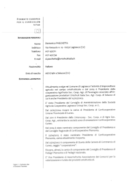
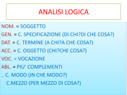
Italy-Spain co-operation 1999-2000
Technical Report UPR/UCa_01_2001
Measurements of breaking waves and bores through a USD
velocity profiler
S. Longo, I.J. Losada, M. Petti, N. Pasotti, J.L. Lara
T = 3.0 s; USDP ->h1030b1.mat; level ->h130b14.dat;
300
250
0°
180°
360°
y (mm)
200
150
100
90°
45°
0°
50
0
-1500
-1000
-500
0
Vx (mm/s)
500
S.W.L.
1000
1500
Department of Civil Engineering
University of Parma, Italy
E.T.S.I.C.C. y P.
Ocean & Coastal Research Group Laboratory
Universidad de Cantabria, Spain
March 2001
co-sponsored by
Ministero dell’Università e della
Ricerca Scientifica (MURST), Italy
Ministerio de Educación y Cultura,
Spain
2
Measurements of breaking waves and bores through a USD velocity
profiler
UPr
UCa
UPr
UCa
Measurements of breaking waves and bores through a USD velocity
profiler
3
REPORT SUMMARY
1. Background and scope of the experiments ...................................................... 7
2. Framework and execution of the study............................................................ 7
3. Experimental set-up ......................................................................................... 8
4. Imposed and measured parameters .................................................................. 9
5. Experimental conditions and test programme ................................................. 9
6. Data analysis .................................................................................................. 10
7. Conclusion ..................................................................................................... 11
8. Acknowledgements........................................................................................ 12
9. General and uncited references...................................................................... 12
10. References................................................................................................... 13
APPENDIX
A1.
A2.
A3.
A4.
A5.
Average operators ...........................................................................................
Characteristics of the instrument ....................................................................
Characteristics of the probes...........................................................................
Volume of measurement .................................................................................
Sources of errors .............................................................................................
Annex 1
Fig. A1Fig. A1Fig. A1Fig. A1Fig. A1Fig. A1-
1 Characteristics of the used US probe.
2 Set-up of a single US probe...................................................................
3 Set-up of three probes............................................................................
4 Set-up of three probes (down view). .....................................................
5 Lay out of the flume. .............................................................................
6 Sections of measurements. ....................................................................
Tab. A1 - 1 DOP 1000 configuration for measurements in Sec. A.Tab. A1 - 2
DOP 1000 configuration for measurements in Sec. B.
Tab. A1 - 3 DOP 1000 configuration for measurements in Sec. C.Tab. A1 - 4
Measuring programme series I.
Tab. A1 - 5 Measuring programme series II (cont.).
Tab. A1 - 6 Measuring programme series III (cont.).
Tab. A1 - 7 Measuring programme series IV (cont.)..............................................
Tab. A1 - 8 Measuring programme Laser series Ia.
4
Measurements of breaking waves and bores through a USD velocity
profiler
Tab. A1 Tab. A1 Tab. A1 Tab. A1 Tab. A1 -
UPr
UCa
9 Measuring programme Laser series Ib. ...............................................
10 Series I ...............................................................................................
11 Series II..............................................................................................
12 Series III.............................................................................................
13 Series IV (cont.).................................................................................
Annex 2
Average water level. Section 1 and 2. T=2.0 s ...............................................
Series I-T=2.0 s..................................................................................................
Average water level. Section 3 (A) and 4 (B). T=2.0 s ..................................
Series I-T=2.0 s............................................................................................... ..
Average water level. Section 5 (C). T=2.0 s...................................................
Series I-T=2.0 s..................................................................................................
Average water level. Section 1 and 2. T=2.0 s ...............................................
Series II-T=2.0 s ................................................................................................
Average water level. Section 3 (A) and 4 (B). T=2.0 s ..................................
Series II-T=2.0 s ................................................................................................
Average water level. Section 5 (C). T=2.0 s...................................................
Series II-T=2.0 s ................................................................................................
Average water level. Section 1 and 2. T=2.5 s ...............................................
Series II-T=2.5 s ................................................................................................
Average water level. Section 3 (A) and 4 (B). T=2.5 s ..................................
Series II-T=2.5 s ................................................................................................
Average water level. Section 5 (C). T=2.5 s...................................................
Series II-T=2.5 s ................................................................................................
Average water level. Section 1 and 2. T=3.0 s ...............................................
Series II-T=3.0 s ................................................................................................
Average water level. Section 3 (A) and 4 (B). T=3.0 s ..................................
Series II-T=3.0 s ................................................................................................
Average water level. Section 5 (C). T=3.0 s...................................................
Series II-T=3.0 s ................................................................................................
Average water level. Section 1 and 2. T=2.0 s ...............................................
Series III-T=2.0 s ...............................................................................................
Average water level. Section 3 (A) and 4 (B). T=2.0 s ..................................
Series III-T=2.0 s ...............................................................................................
Average water level. Section 1 and 2. T=2.5 s ...............................................
Series III-T=2.5 s ...............................................................................................
Average water level. Section 3 (A) and 4 (B). T=2.5 s ..................................
Series III-T=2.5 s ...............................................................................................
Average water level. Section 1 and 2. T=3.0 s ...............................................
Series III-T=3.0 s ...............................................................................................
UPr
UCa
Measurements of breaking waves and bores through a USD velocity
profiler
5
Average water level. Section 3 (A) and 4 (B). T=3.0 s ..................................
Series III-T=3.0 s ...............................................................................................
Average water level. Section 1 and 2. T=2.0 s ...............................................
Series IV-T=2.0 s ...............................................................................................
Average water level. Section 3 (A) and 4 (B). T=2.0 s ..................................
Series IV-T=2.0 s ...............................................................................................
Average water level. Section 1 and 2. T=2.5 s ...............................................
Series IV-T=2.5 s ...............................................................................................
Average water level. Section 3 (A) and 4 (B). T=2.5 s ..................................
Series IV-T=2.5 s ...............................................................................................
Average water level. Section 1 and 2. T=3.0 s ...............................................
Series IV-T=3.0 s ...............................................................................................
Average water level. Section 3 (A) and 4 (B). T=3.0 s ..................................
Series IV-T=3.0 s ...............................................................................................
Noise evaluation in Section A. .......................................................................
Series IV .............................................................................................................
Noise evaluation in Section B.........................................................................
Series IV .............................................................................................................
Noise evaluation in Section C.........................................................................
Series IV .............................................................................................................
Horizontal velocity profiles. Sections A and B. T=2.0 s ................................
Series IV-T=2.0 s ...............................................................................................
Horizontal velocity profiles. Sections A and B. T=2.5 s ................................
Series IV-T=2.5 s ...............................................................................................
Horizontal velocity profiles. Sections A and B. T=3.0 s ................................
Series IV-T=3.0 s ...............................................................................................
Phasic and mean velocity profiles. Section A. T=2.0 s ..................................
Series IV-T=2.0 s ...............................................................................................
Phasic and mean velocity profiles. Section B. T=2.0 s ..................................
Series IV-T=2.0 s ...............................................................................................
Phasic and mean velocity profiles. Section A and B. T=2.5 s........................
Series IV-T=2.5 s ...............................................................................................
Phasic and mean velocity profiles. Section A. T=3.0 s ..................................
Series IV-T=3.0 s ...............................................................................................
Phasic and mean velocity profiles. Section B. T=3.0 s ..................................
Series IV-T=3.0 s ...............................................................................................
Laser measurements phase average velocities at different levels. Each curve
has been shifted upward by 0.1 with respect to the previous. ........................
Laser series ........................................................................................................
Laser measurements phase average fluctuations at different levels. Each
curve has been shifted upward by 0.01 with respect to the previous. ............
Laser series ........................................................................................................
6
Measurements of breaking waves and bores through a USD velocity
profiler
UPr
UCa
Phase average Reynold’s stress at different levels. Each curve has been
shifted upward by 0.001 with respect to the previous. ...................................
Laser series ........................................................................................................
Laser measurements. Velocity profiles. T=3.0 s ............................................
Laser series ........................................................................................................
Annex 3
List and structure of data files
UPr
UCa
Measurements of breaking waves and bores through a USD velocity
profiler
7
1. Background and scope of the experiments
Fluid velocity measurements under waves and bores are essential to validate
existing models or to build up new models. Laser Doppler Velocimetry (LDV) is
widely used with several limitations due to bubble presence if breaking occurs.
Also Hot Wire and Hot Film anemometry is often used in the labs, as well as
Particle Image Velocimetry (PIV) with good results and with several other
limitations.
The present experiments are focused on the study of the time dependent
velocity in breaking waves and subsequent bores in shallow water using a
relatively recent technique based on ultrasound. Velocity profiles parallel and
orthogonal to the bottom are measured using a Doppler Ultrasonic Technique.
The experimental research was carried out in June and July 2000.
The data have been validated and partially elaborated, and are available for a
more detailed verification of the technique in unsteady free surface flows.
2. Framework and execution of the study
The experimental investigation was part of the Italy-Spain 2000 Co-operation
programme and was funded by the Ministero dell’Università e delle Ricerca
Scientifica (MURST), Italy, and by the Ministerio de Educación y Cultura,
Spain.
The experiments were carried out in the small channel of the Ocean &
Coastal Research Group Laboratory, E.T.S.I.C.C. y P., Universidad de Cantabria
in Santander, Spain, in the weeks from 10th June to 7th July 2000.
The experiment execution and data analysis was conducted by the following
research team:
Sandro Longo, University of Parma, Italy
Marco Petti, University of Udine, Italy
Nicoletta Pasotti, University of Udine, Italy
Inigo Losada, University of Santander, Spain
Javier Lopez Lara, University of Santander, Spain
8
Measurements of breaking waves and bores through a USD velocity
profiler
UPr
UCa
3. Experimental set-up
The experiments were carried out in the small flume in the laboratory of the
Ocean and Coastal Research Group at the Universidad de Cantabria of
Santander. In Fig.A1-5 and Fig. A1-6 (Annex 1) the general outline of the flume
and the measurement sections are shown.
Different apparatus were used in the experiments, as follows:
Wave flume with wave paddle.
Control and acquisition data equipment.
Water level gauges.
Laser Doppler Velocimeter.
Digital video camera.
Digital photographic camera.
The wave flume is 24.00 m long, 0.58 m wide and 0.80 m deep. Glass
sidewalls and bottom of the tank are distributed in 20.00 m, to have a visual
access to the wave development.
Waves were generated with a piston type paddle with AWACS (Active Wave
Absorption Control System) to correct reflected waves. The paddle is made of
stainless steel moved by a hydraulic piston. Its frontal surface is covered with a
10 mm thick PVC plate, where two water surface gauges are located to identify
water surface elevation. Its technical characteristics are:
Inertial mass: 20 N s2/m.
Maximum horizontal stroke: 1000 mm.
Frontal surface: 0.58 m2.
Width: 0.58 m.
Height: 0.995 m.
Maximum strength: 5031 N.
Oil-hydraulic group power: 10 KW.
Paddle generation program and data acquisition procedure used have been
developed by the Coastal and Ocean Research group. This procedure includes
wave generation and gauges calibration procedure. Data have been store in a PC
computer where a digital-analogic board is incorporated.
Firstly, a plastic glass false bottom has been installed in the wave tank to
create a uniform slope of 1 on 20. The still water depth in the constant-depth
region of the tank was 0.4 m in most experiments. The slope has been sealed to
the tank walls filling the gap between the edges of the slope and the sidewalls
with silicone.
UPr
UCa
Measurements of breaking waves and bores through a USD velocity
profiler
9
DHI resistive type water level gauges were located on an instrument platform,
which can slide along the top of the tank on two rails.
A DANTEC LDV (Laser Doppler Velocimeter) was used to take velocity
measurements. It is a backscatter, four-beams system with a 6 W ion-argon laser
generator refrigerated by water. A 30.00 m optical fiber carries laser beams from
an optical system to the measurements location, where it is fixed into a two
dimensional programmable transverse system. Data were also stored in a PC
computer.
A Ultrasound Doppler Velocity Profiler DOP1000 (www.signalprocessing.com) was used to take velocity measurements in three sections, with
three probes per section.
4. Imposed and measured parameters
Several combinations of sinusoidal waves were realised in the flume by
imposing a required piston movement.
The following parameters were measured:
• Water level in five sections
• Water velocity in three sections using USDP
• Water velocity in one section using LDV.
The frequency of acquisition was equal to 180 Hz for water level, from ∼10 to
∼30 Hz (∼10 to ∼30 velocity profiles per second) for USDP, varying for LDV
(data were stored with frequency related to the occurrence of validated burst),
with maximum value around 2 kHz.
The data were originally stored in ASCII format for the water level gauges,
ASCII format for LDV and in binary format for the DOP1000. After a
preliminary elaboration, the latter are also available in binary Matlab files
form.
5. Experimental conditions and test programme
The experimental programme consisted of three different period sinusoidal
waves and two wave height. The still water level in the horizontal bottom part of
the flume varies from 40 cm to 36 cm, in order to obtain wave breaking in the
first section of measurement of the fluid velocity. The generated waves are linear
or corrected to the 5th order. A long wave absorbing system is active during wave
generation.
Tests carried out were:
10
Measurements of breaking waves and bores through a USD velocity
profiler
UPr
UCa
Series I
5th order waves, single wave period T=2.0 s, wave height H=12 cm, still water
level = 40 cm. Fluid velocity measurements through UDVP in three sections.
Series II
Linear waves, three wave periods T=2.0; 2.5; 3.0 s, H=12 cm, s.w.l.=40 cm.
Fluid velocity measurements through UDVP in three sections.
Series III
5th order waves, three wave periods T=2.0; 2.5; 3.0 s, H=10 cm, s.w.l.=37 cm.
Fluid velocity measurements through UDVP in three sections.
Series IV
5th order waves, three wave periods T=2.0; 2.5; 3.0 s, H=10 cm, s.w.l.=36 cm.
Fluid velocity measurements through UDVP in two sections.
Laser Series
5th order waves, three wave periods T=3.0 s, H=10 cm, s.w.l.=37 cm. Fluid
velocity measurements through UDVP in one sections. 2-D LDV measurements
in 21 points in the vertical of one section.
6. Data analysis
Data have been analysed in the time domain. Water level elevation measured
by the 5 probes (except for a subset of tests where the last probe was dry most of
the time), UDVP velocity profiles and LDV measurements have been averaged
in phase using a Variable Time Interval Average (VITA) in order to obtain their
evolution during one period. The VITA requires a trigger event. It has been
chosen as the instant of maximum water level. Moreover only those short time
series lasting for a time equal to T ± 0.02T have been selected and averaged.
The results are reported in Annex 2. The dashed lines represent the maximum
and minimum level recorded and thus a measurement of the variance. The
variance is modest for non-breaking waves, recorded in Sec.1 and 2, and strongly
increases after breaking (subsequent sections).
The UDVP velocity profiles, obtained applying the techniques reported in
Appendix, have been averaged in phase choosing as first profile in the period the
nearest to the instant of trigger (the instant of maximum water level in the
section).
The results are reported in Annex II only for the Measurement Series IV,
characterised by the maximum data rate of UDVP (≈30 profiles per second per
UPr
UCa
11
Measurements of breaking waves and bores through a USD velocity
profiler
each probe). Also AVI files have been obtained containing the animation of
velocity profiles.
UDVP velocity profiles have been also time averaged in order to obtain the
mean fluid velocity. The classical undertow is evident in all sections.
The aim of LDV measurements was the comparison of results with those
obtained through USDP. Unfortunately the USDP signal was useless during
Laser Series. Anyway the LDV data have been analysed.
Phase averaged velocity profiles were calculated at each level from the
bottom in Section 3 (A). Turbulent oscillations u '( y, t ) along the main flow
direction have been obtained by subtracting the phase-averaged value u% ( y, t )
from the instantaneous velocity measured u ( y, t ) :
u '( y, t ) = u ( y, t ) − u% ( y, t )
.
v '( y, t ) = v( y, t ) − v% ( y, t )
(1)
The phase averaged values were obtained using a VITA technique triggering
to the maximum horizontal velocity.
The phase average horizontal and vertical velocity and turbulent fluctuations are
' v ' profiles are reported for the 20
reported in Annex II. Also the cross product u²
useful levels over the bottom where LDV measurements took place.
7. Conclusion
UDVP technique has several advantages respect to other fluid velocity
measurements. It can give information on spatio-temporal velocity, with data rate
virtually independent on seeding concentration. It can also be used in opaque
fluids. The error is strictly related to the accuracy of set-up, and can be reduced
to less than 5%.
The present limits are essentially due to the low data rate, which allows at
most macro-turbulence measurements. The low data rate is intrinsic in the carrier
celerity, around 1000 m/s. The system has the disadvantage of no data validation,
and of a large volume of measurements, although this last limit can be eliminated
using some focussed probes. The absence of data validation can generate error
due to aliasing: if the Doppler frequency is out of the bandwidth, the spectrum is
aliasiazed and the estimated velocity is not correct. It is an important limit in high
turbulence flows.
In the flow field analysed in the present experimental activity, the
instrument had good performances especially in situations where LDV
measurements are not useful, as in bores after breaking.
12
Measurements of breaking waves and bores through a USD velocity
profiler
UPr
UCa
8. Acknowledgements
This work is undertaken as part of Italy-Spain Co-operation Project, 2000.
Nicoletta Pasotti has also partially been supported by MAST III - SASME
Project (“Surf and Swash Zone Mechanics”) founded by the Commission of the
European Communities, Directorate General Research and Development under
contract no. MAS3-CT97-0081. We wish to express our thanks to the technicians
and to the staff of the Ocean & Coastal Research Group Laboratory, in
Santander, for their valuable collaboration in carrying out experiments.
9. General and uncited references
Antoine, Y. And Lebouché, M., 1998. Détermination de vitesses de glissement
lors de l’écoulement d’une suspension non newtonienne par utilisation de la
vélocimétrie ultrasonore à effet Doppler. C.R.Acad.Sci. Paris, t.326, Série II
b, p. 367-372.
Austin, J.C. and Challis, R.E., 1999. Ultrasonic propagation through aqueous
kaolin suspensions during degassing. Ultrasonics, 37:299-302.
Battjes, J. A and Sakai, T., 1980. Velocity field in a steady breaker. J. Fluid
Mech. 111: 421-437.
Costigan, G. and Whalley, P.B., 1997. Measurements of the speed of sound in
air-water flows. Chem. Engineering Journal, 66: 131-135.
Hinze, J.O., 1975. Turbulence. McGraw-Hill series in mechanical engineering.
Inoue, Y., Yamashita, S. and Kumada, M., 1999. An experimental study on a
wake behind a torus using the UVP monitor. Exp. In Fluids, 26: 197-207.
Kikura, H., Takeda, Y. And Durst, F., 1999. Velocity profile measurement of the
Taylor vortex flow of a magnetic fluid using the ultrasonic Doppler method.
Exp. In Fluids, 26: 208-214.
Laborde, J.-L., Hita, A., Caltagirone, J.-P. and Gerard, A., 2000. Fluid dynamics
phenomena induced by power ultrasounds. Ultrasonics, 38: 297-300.
Lemmin, U. and Rolland, T., 1997. Acoustic velocity profiler for laboratory and
field studies. J. of Hydraulic Engineering, Vol. 123, No. 12, pp. 1089-1098.
Marcos, A.-G., 1999. Etude d’un Vélocimètre Doppler Ultrasonore (Signal
Precessing) pour son utilisation en canal à houle.Master Report, Groupe
Mécanique des Fluides & Génie Côtier, D.E.A. Énergétique et
Aérothermochimie Option Combustion et Moteur, Université de Caen, France
(in french).
Nielsen, K.D., Weber, L.J. and Muste, M., 1999. Capabilities and limits for ADV
measurements in bubbly flows. XXVIII IAHR Congress, Graz.
Papoulis, A., 1965. Probability, random variables and stochastic problems.
McGraw-Hill, NY.
Peschard, I., Le Gal, P. and Takeda, Y., 1999. On the spatio-temporal structure of
cylinder wakes. Exp. In Fluids, 26: 188-196.
UPr
UCa
Measurements of breaking waves and bores through a USD velocity
profiler
13
Petti, M., Longo, S., Sadun, S. and Tirindelli, M., 1998. Swash zone
hydrodynamics on a 1:10 bottom slope: laboratory data. SASME Report
FIUD-01-98, Univ.of Florence.
Signal Processing, 1998. Manual for DOP1000.
Rodriguez, A., Sanchez-Arcilla, A., Redondo, J.M. and Mosso, C., 1999.
Macroturbulence measurements with electromagnetic and ultrasonic sensors:
a comparison under high-turbulent flows. Exp. In Fluids, 27: 31-42.
Rolland, T. and Lemmin, U., 1997. A two-component acoustic velocity profiler
for use in turbulent open channel flow. J. of Hydraulic Research, Vol. 35, No.
4, pp. 545-561.
Schouveiler, L., Le Gal, P., Chauve, M.P. and Takeda, Y., 1999. Spiral and
circular waves in the flow between a rotating and a stationary disk. Exp. In
Fluids, 26: 179-187.
Wunderlich, Th. And Brunn, P.O., 2000. A wall layer correction for ultrasound
measurement in tube flow: comparison between theory and experiment. Flow
Meas. and Instrum., 11: 63-69.
Wunderlich, Th. And Brunn, P.O., 1999. Ultrasound pulse Doppler method as
viscometer for process monitoring. Flow Meas. and. Instr., 10, pp. 201-205.
Wunenburger, R., Andreotti, B. and Petitjeans, P., 1999. Influence of precession
on velocity measurements in a strong laboratory vortex. Exp. In Fluids, 27:
181-188.
10. References
Blackwelder, R.F. and Kaplan, R.E., 1976. On the wall structure of the turbulent
boundary layer. J. Fluid Mech., 76, 80-112.
Kikura, H., Takeda, Y. And Durst, F., 1999. Velocity profile measurement of the
Taylor vortex flow of a magnetic fluid using the ultrasonic Doppler method.
Exp. In Fluids, 26: 208-214.
Nikora, V.I. and Goring, D.G., 1998. ADV measurements of turbulence: can we
improve their interpretation ?. J. of Hydraulic Engineering, Vol. 124, No. 6,
pp. 630-634.
Petti, M. and Longo, S., 2001. Turbulence experiments in the swash zone. Coast.
Engineering, Vol.43-1, pp.1-24.
Takeda, Y., 1999. Ultrasonic Doppler method for velocity profile measurement
in fluid dynamics and fluid engineering. Exp. In Fluids, 26: 177-178.
APPENDIX
App. 2
Measurements of breaking waves and bores through a USD velocity
profiler
UPr
UCa
UPr
UCa
A1.
A2.
A3.
A4.
A5.
Measurements of breaking waves and bores through a USD velocity
profiler
App. 3
Average operators .................................................................................4
Characteristics of the instrument ..........................................................5
Characteristics of the probes.................................................................5
Volume of measurement.......................................................................5
Sources of errors ...................................................................................6
App. 4
A1.
Measurements of breaking waves and bores through a USD velocity
profiler
UPr
UCa
Average operators
There are several operators used for periodic signals. The ensemble or phase
average η% (t ) of a time series is expressed as:
η% (t ) =
1
N
N −1
∑η (t + kT )
0≤t<T
(A1)
k =0
where η (t ) represents instantaneous values, N is the number of waves in the
chosen time interval and T is the period. This operator is highly sensitive to small
fluctuations of the period, due for example to a frequency modulating effect.
If a well-identified trigger is available, the conditional average is expressed as:
η% (t ) =
1
N
N −1
∑η ( t + t )
k
k =0
0 ≤ t < min(T)
(A2)
where tk is the instant of trigger of the k-cycle and min(T) is the minimum time
period in the series of N cycles. The conditional average is widely known as the
Variable Interval Time Average (VITA, see Blackwelder and Kaplan, 1976). A
more correct and unbiased result can be obtained stretching the data of each cycle
(the time period of each cycle, equal to (tk- tk-1) is not constant) before averaging
in order to extend it all over the mean period. Such a technique is equivalent to
the demodulation process in the time-domain of a weak-modulated (in
frequency) signal (Petti and Longo, 2001).
If the value of time series is not defined during some time intervals (e.g.
Eulerian fluid velocity is strictly related to mass presence in the point of
measurements, and is not defined during mass absence) we can define a phasic
average:
ηˆ =
∑ ∫ η ( t ) dt
∑ ∆T
i ∆Ti
(A3)
i
i
where ∆Ti are the time steps during water presence. This last operator is
particularly important in the analyses of our data because in some sections of
measurements the water is often absent.
For completeness, the well-known time average operator is reported:
< η >=
1
T
T
∫ η ( t ) dt ,
0
(A4)
UPr
UCa
Measurements of breaking waves and bores through a USD velocity
profiler
App. 5
with T the period of time averaging.
All the above-defined operators are linear and can be applied in sequence without
rank.
A2.
Characteristics of the instrument
DOP1000 is an instrument for the measurement of fluid velocity in several
measuring volumes along the beam of a piezo-electric transducer, working as
emitter and receiver. It is based on pulsed ultrasonic Doppler effect. The source
of signal is pressure wave generated by an emitter with frequency ranging from 1
to 10 MHz. The signal scattered by seeding particles and/or eddies is elaborated
to detect particle position using the travel time of the signal and the echo, and
particle velocity using the frequency shift of the echo. This technique has some
major advantages respect to traditional techniques (e.g. Laser Doppler
Velocimetry LDV, Particle Image Velocimetry PIV, Electro Magnetic
Flowmeter EMF), as the spatio-temporal information about the flow field. See
Takeda, 1999, for accurate description of these advantages.
A3.
Characteristics of the probes
The source of pressure waves is a piezo electric quartz transducer driven by
electronics. The pressure field is strictly related to the geometry of the
transducer. In general it is possible to distinguish a near field, (Fresnel zone)
where the acoustic field is cylindrical (if the source probe is circular) and a far
field where the acoustic field has several lobes. See Fig. A1-1.
The probes used are piezoelectric transducers working at 1 MHz with plastic
housing 18 mm in diameter and active element diameter of 14 mm. The near
field extends for 32 mm and the divergence angle is 15°. The ultrasonic beam
passing through plexiglass modify its path, due to refraction in the medium
having different acoustic impedance.
To investigate a 2-D flow fields, at least two probes have to be set-up; usually
three probes are used. See Fig.A1-2 for the single probe arrangement and Fig.
A1-3 for the three probes set-up.
A4.
Volume of measurement
For the probe we used, the near field is 32 mm wide, and the total angle of
divergence is of 15°. This behaviour generates relatively wide and thin volumes
of measurements, enlarged far from the probe.
The volume of measurement depends on the probe characteristics.
App. 6
A5.
Measurements of breaking waves and bores through a USD velocity
profiler
UPr
UCa
Sources of errors
Several tests on performances of ADV (measurement of three velocity
components in a single volume) are available. The main source of errors,
especially in turbulence measurements, is the Doppler noise. It is probably due to
multiple particles or micro eddies present in the volume of measurement, which
scatter echoes broadening the spectral peak. Tests conducted by Nikora and
Goring , 1998, give the following main results:
Spectra and probability distributions indicate that Doppler noise is essentially
a Gaussian white noise.
Doppler noise depends on the seeding particles, and is higher for bubbles.
The two Authors also suggest a technique to estimate the Doppler noise
influence on turbulent characteristics, based on measuring Doppler signal with
the instrument set-up in the same condition of the experiment (same velocity
range, pulse repetition frequency etc. ) but in still water having the same seeding
characteristics of the water used in the experiments. The two velocity
components can be expressed as a function of the velocity measured along the
beams and of their noise:
(u , v) = f (ui , N i )
(A5)
with f determined by the geometry of the probes, ui are the true values of the
velocity components along the i-beam and Ni is the noise along the i-beam. The
transformation can be written as:
 u1 + N1 
u 

  = A
v 
u 2 + N 2 
(A6)
The expected values are simply:
u
 u1 + N1 
  = A

v 
 u2 + N 2 
(A7)
and the estimated variances are:
 u '2 
 u '12 + N '12
 2  = A 2
2
 v' 
 u '2 + N '2



(A8)
UPr
UCa
Measurements of breaking waves and bores through a USD velocity
profiler
App. 7
under the hypothesis that the velocity-noise correlation are zero. The
estimators of the true components can be obtained as:
ui = u im − N i
(A9)
2
u 'i2 = u 'im
− N 'i2
where the subscript m indicates the measured value.
The mean errors and the error variances have been computed for homogeneus
conditions of acquisition (same spatial resolution, PRF) in still water conditions,
and are reported in Annex 2.
v
u
Wave direction
v1
α
3
1
2
Fig. App.1. Reference system
The velocity components in x and y directions can be obtained measuring
velocity components along the beam axes (see reference system):
u1 = −usinα − v cos α
u 3 = usinα − v cos α
(A10)
u 2 = −v
The system is over constrained. The minimum error is obtained using the first
two relationships to determine the u component, and the third relationship for the
App. 8
Measurements of breaking waves and bores through a USD velocity
profiler
UPr
UCa
vertical velocity component. Similar transformations can be obtained for the
variances:
u±'12 − u±'32
²
u 'v ' =
sin 2α
u±'2 + u±'32 − 2u±'22 cos 2 α
u±'2 = 1
2sin 2 α
v±'2 = u±'2
(A11)
2
The measured noise and its STD has been computed in the three sections and
are reported in Annex 2.
ANNEX 1
A1 - 2
Measurements of breaking waves and bores through a USD velocity
profiler. Annex 1
UPr
UCa
UPr
UCa
Measurements of breaking waves and bores through a USD velocity
profiler. Annex 1
A1 - 3
Fig. A1Fig. A1Fig. A1Fig. A1Fig. A1Fig. A1-
1 Characteristics of the used US probe................................................... 7
2 Set-up of a single US probe................................................................. 8
3 Set-up of three probes.......................................................................... 9
4 Set-up of three probes (down view). ................................................. 10
5 Lay out of the flume. ......................................................................... 12
6 Sections of measurements. ................................................................ 12
Tab. A1 Tab. A1 Tab. A1 Tab. A1 Tab. A1 Tab. A1 Tab. A1 Tab. A1 Tab. A1 Tab. A1 Tab. A1 Tab. A1 Tab. A1 -
1 DOP 1000 configuration for measurements in Sec. A. ..................... 4
2 DOP 1000 configuration for measurements in Sec. B. ..................... 5
3 DOP 1000 configuration for measurements in Sec. C. ..................... 6
4 Measuring programme series I. ....................................................... 13
5 Measuring programme series II (cont.). .......................................... 14
6 Measuring programme series III (cont.). ......................................... 16
7 Measuring programme series IV (cont.).......................................... 18
8 Measuring programme Laser series Ia............................................. 20
9 Measuring programme Laser series Ib. ........................................... 21
10 Series I ........................................................................................... 22
11 Series II.......................................................................................... 23
12 Series III......................................................................................... 24
13 Series IV (cont.)............................................................................. 25
A1 - 4
Measurements of breaking waves and bores through a USD velocity
profiler. Annex 1
DOP1000 version .........................
Data type ...............................
Emitting frequency ......................
Emitting power ........................
Pulse repetition frequency ............
Burst length ..........................
Resolution ..............................
Sensitivity .............................
Number of emission pro profiles .........
Doppler scale factor ....................
Maximum velocity ......................
Minimum velocity ......................
Velocity offset (coded and in mm/s) ...
Memory size .............................
Number of bytes pro profile ...........
Skip profile ..........................
Number of channels ......................
First channel at ......................
First recorded channel ................
Last recorded channel..................
Anterior wall at channel ..............
Posterior wall at channel .............
Cursor at channel .....................
Selected filter type ....................
Zero values ...........................
Number of profiles used for filtering .
FFT channel position ....................
FFT window ............................
FFT number of points ..................
Unit ....................................
Doppler angle .........................
Sound velocity.........................
TGC mode ................................
TGC start value .......................
TGC end value .........................
Trigger .................................
Trigger mode ..........................
Trigger delay .........................
Number of profiles pro sequences ......
Number of sequences ...................
Multilplexer ............................
Recorded profiles on transducer 1 .....
Recorded profiles on transducer 2 .....
Recorded profiles on transducer 3 .....
UPr
UCa
5.23
Velocity
1.0 MHz
Medium
3125 Hz,320 µs ,240 mm
8
cycles
2.0 µs,1.50 mm
Medium
64
31.2 ms
2
1171.50
mm/s
-1171.50
mm/s
0
0
mm/s
20000 624000 ms
164
0
.0 ms
154
.0 µs,.0 mm
1
.0 µs,.0 mm
154
306.0 µs,229.5 mm
8
14.0 µs,10.5 mm
10
18.0 µs,13.5 mm
10
18.0 µs,13.5 mm
none
included
2
19
28.5
Hamming
128
US axis
0
degrees
1500
m/s
slope
18
dB
40
dB
On
Waiting for +
0
.0 ms
20000 624000 s
1
Multiplex on
1
31.2
ms
1
31.2
ms
1
31.2
ms
Tab. A1 - 1 DOP 1000 configuration for measurements in Sec. A.
UPr
UCa
Measurements of breaking waves and bores through a USD velocity
profiler. Annex 1
DOP1000 version .........................
Data type ...............................
Emitting frequency ......................
Emitting power ........................
Pulse repetition frequency ............
Burst length ..........................
Resolution ..............................
Sensitivity .............................
Number of emission pro profiles .........
Doppler scale factor ....................
Maximum velocity ......................
Minimum velocity ......................
Velocity offset (coded and in mm/s) ...
Memory size .............................
Number of bytes pro profile ...........
Skip profile ..........................
Number of channels ......................
First channel at ......................
First recorded channel ................
Last recorded channel..................
Anterior wall at channel ..............
Posterior wall at channel .............
Cursor at channel .....................
Selected filter type ....................
Zero values ...........................
Number of profiles used for filtering .
FFT channel position ....................
FFT window ............................
FFT number of points ..................
Unit ....................................
Doppler angle .........................
Sound velocity.........................
TGC mode ................................
TGC start value .......................
TGC end value .........................
Trigger .................................
Trigger mode ..........................
Trigger delay .........................
Number of profiles pro sequences ......
Number of sequences ...................
Multilplexer ............................
Recorded profiles on transducer 1 .....
Recorded profiles on transducer 2 .....
Recorded profiles on transducer 3 .....
A1 - 5
5.23
Velocity
1.0 MHz
medium
2906 Hz,344 µs,258 mm
8
cycles
2.0 µs,1.50 mm
medium
64
33.1 ms
2
1089.75
mm/s
-1089.75
mm/s
0
0
mm/s
20000 662000 ms
176
0
.0 ms
166
.0 µs,.0 mm
1
.0 µs,.0 mm
166
330.0 µs,247.5 mm
8
14.0 µs,10.5 mm
10
18.0 µs,13.5 mm
10
18.0 µs,13.5 mm
none
included
2
19
28.5
Hamming
128
US axis
0
degrees
1500
m/s
slope
14
dB
40
dB
On
Waiting for +
0
.0 ms
20000 662000 s
1
Multiplex on
1
33.1
ms
1
33.1
ms
1
33.1
ms
Tab. A1 - 2 DOP 1000 configuration for measurements in Sec. B.
A1 - 6
Measurements of breaking waves and bores through a USD velocity
profiler. Annex 1
DOP1000 version .........................
Data type ...............................
Emitting frequency ......................
Emitting power ........................
Pulse repetition frequency ............
Burst length ..........................
Resolution ..............................
Sensitivity .............................
Number of emission pro profiles .........
Doppler scale factor ....................
Maximum velocity ......................
Minimum velocity ......................
Velocity offset (coded and in mm/s) ...
Memory size .............................
Number of bytes pro profile ...........
Skip profile ..........................
Number of channels ......................
First channel at ......................
First recorded channel ................
Last recorded channel..................
Anterior wall at channel ..............
Posterior wall at channel .............
Cursor at channel .....................
Selected filter type ....................
Zero values ...........................
Number of profiles used for filtering .
FFT channel position ....................
FFT window ............................
FFT number of points ..................
Unit ....................................
Doppler angle .........................
Sound velocity.........................
TGC mode ................................
TGC start value .......................
TGC end value .........................
Trigger .................................
Trigger mode ..........................
Trigger delay .........................
Number of profiles pro sequences ......
Number of sequences ...................
Multilplexer ............................
Recorded profiles on transducer 1 .....
Recorded profiles on transducer 2 .....
Recorded profiles on transducer 3 .....
UPr
UCa
5.23
Velocity
1.0 MHz
Medium
3125 Hz,320 µs,240 mm
8
cycles
1.0 µs,.75 mm
Medium
64
31.2 ms
2
1171.50
mm/s
-1171.50
mm/s
0
0
mm/s
20000 624000 ms
234
0
.0 ms
224
.0 µs,.0 mm
1
.0 µs,.0 mm
224
223.0 µs,167.2 mm
8
7.0 µs,5.2 mm
10
9.0 µs,6.7 mm
10
9.0 µs,6.7 mm
None
Included
2
19
14.2
Hamming
128
US axis
0
degrees
1500
m/s
slope
-3
dB
40
dB
On
Waiting for +
0
.0 ms
20000 624000 s
1
Multiplex on
1
31.2
ms
1
31.2
ms
1
31.2
ms
Tab. A1 - 3 DOP 1000 configuration for measurements in Sec. C.
UPr
UCa
Measurements of breaking waves and bores through a USD velocity
profiler. Annex 1
A1 - 7
Ultrasound
beam
Probe
b
d
Frequency
(MHz)
1
Piezo
diameter
(mm)
14
Plastic
housing d
(mm)
18
b (mm)
76
Fig. A1- 1 Characteristics of the used US probe.
Near field Z Divergence
(mm)
degrees
32
15
A1 - 8
Measurements of breaking waves and bores through a USD velocity
profiler. Annex 1
20°
4 Ø4 x 20
brass
50
PVC
25
80
O- ring
70
40
Ø1
7
8.1
160°
10
34.6
13.1
PVC ring
Ø4
0
Ø1
9
10
3 Ø4 x 20
brass
70
Ø1
bell mouth
Ø5
80
Ø40
4
Ø4
PVC ring
50
4
US probe
Fig. A1- 2 Set-up of a single US probe.
Ø19
UPr
UCa
UPr
UCa
Measurements of breaking waves and bores through a USD velocity
profiler. Annex 1
Plexiglas false bottom
40°
70
41
bell mouth
66
25
Ø 17
O- ring
Fig. A1- 3 Set-up of three probes.
Ø 18.1
A1 - 9
A1 - 10
Measurements of breaking waves and bores through a USD velocity
profiler. Annex 1
Fig. A1- 4 Set-up of three probes (down view).
UPr
UCa
UPr
UCa
Measurements of breaking waves and bores through a USD velocity
profiler. Annex 1
A1 - 11
A1-12
UPr
UCa
Measurements of breaking waves and bores through a USD velocity profiler. Annex 1.
WAVE BOARD
WG1
WG2
WG3
WG4
A
Fig. A1- 5 Lay out of the flume.
LDV measurement
section
WG3
WG4
A
WG5
B
C
Fig. A1- 6 Sections of measurements.
WG5
B
C
Water level elevation files
date
Test
(UDVP
file)
condition
WG3
WG4
WG5
sec. A
sec. B
sec. C
8.0
13.0
14.2
15.35
40
15
9
3.3
WG1
WG2
2.5
H=12 cm
40
T=2.0 s
H1220a1.dat
still water depth (cm)
H1220a
27.6.2000
H1220b
5th order
H1220b1.dat
generation waves
H1220b2.dat
H1220b3.dat H1220b4.dat H1220b5.dat velocity meas. in section B
27.6.2000
H1220c
H1220c1.dat
H1220c2.dat
H1220c3.dat
H1220c4.dat H1220c5.dat velocity meas. in section C
LIV0011.dat
LIV0012.dat
LIV0013.dat
LIV0014.dat
26.6.2000
27.6.2000
ca260600.cal
Remarks:
distance from the paddle
(m)
26.6.2000
26.6.2000
H1220a2.dat H1220a3.dat H1220a4.dat
description
H1220a5.dat velocity meas. in section A
LIV0015.dat
zero calibration
calibration file
LEV0021.dat LEV0022.dat LEV0023.dat LEV0024.dat LEV0025.dat zero calibration
27.6.2000
ca270600.cal
calibration file
Tab. A1 - 4 Measuring programme series I.
Measurements of breaking waves and bores through a USD velocity profiler. Annex 1.
A1-13
UPr
UCa
A1-14
UPr
UCa
Measurements of breaking waves and bores through a USD velocity profiler. Annex 1.
Water level elevation files
date
test
(UDVP
file)
27.6.2000
L1220a
30.6.2000
L1220a_2
WG3
WG4
WG5
sec. A
sec. B
sec. C
8.0
13.0
14.2
15.35
40
15
9
3.3
condition
WG1
WG2
H=12 cm
2.5
linear generation
waves
40
description
distance from the paddle
(m)
still water depth (cm)
Ll1220a1.dat Ll1220a2.dat Ll1220a3.dat Ll1220a4.dat Ll1220a5.dat
velocity meas. in section A UDVP not useful
L1220a1.dat
L1220a2.dat
L1220a3.dat
L1220a4.dat
L1220a5.dat
velocity meas. in section A
T=2.0 s
28.6.2000
L1220b
L1220b1.dat
L1220b2.dat
L1220b3.dat
L1220b4.dat
L1220b5.dat
velocity meas. in section B
28.6.2000
L1220c
L1220c1.dat
L1220c2.dat
L1220c3.dat
L1220c4.dat
L1220c5.dat
velocity meas. in section C
27.6.2000
L1225a
L1225a1.dat
L1225a2.dat
L1225a3.dat
L1225a4.dat
L1225a5.dat
velocity meas. in section A
28.6.2000
L1225b
L1225b1.dat
L1225b2.dat
L1225b3.dat
L1225b4.dat
L1225b5.dat
velocity meas. in section B
28.6.2000
L1225c
L1225c1.dat
L1225c2.dat
L1225c3.dat
L1225c4.dat
L1225c5.dat
velocity meas. in section C
T=2.5 s
Remarks:
Tab. A1 - 5 Measuring programme series II (cont.).
substitutes
L1220a
Water level elevation files
date
test
(UDVP
file)
27.6.2000
L1230a
30.6.2000
L1230a_2
WG3
WG4
WG5
sec. A
sec. B
sec. C
condition
WG1
WG2
H=12 cm
2.5
8.0
13.0
14.2
15.35
linear generation
waves
40
40
15
9
3.3
description
distance from the paddle
(m)
still water depth (cm)
LI1230a1.dat LI1230a2.dat LI1230a3.dat LI1230a4.dat LI1230a5.dat velocity meas. in section A
UDVP not useful
L1230a1.dat L1230a2.dat
L1230a3.dat L1230a4.dat
substitutes
L1230a
L1230a5.dat
velocity meas. in section A
velocity meas. in section B
T=3.0 s
28.6.2000
L1230b
L1230b1.dat L1230b2.dat
L1230b3.dat
L1230b4.dat L1230b5.dat
28.6.2000
L1230c
L1230c1.dat L1230c2.dat
L1230c3.dat
L1230c4.dat
L1230c5.dat velocity meas. in section C
LIV0031.dat LIV0032.dat
LIV0033.dat
LIV0034.dat
LIV0035.dat
28.6.2000
Remarks:
28.6.2000
ca280600.cal
zero calibration
calibration file
Measuring programme series II (cont’d.).
Measurements of breaking waves and bores through a USD velocity profiler. Annex 1.
A1-15
UPr
UCa
A1-16
UPr
UCa
Measurements of breaking waves and bores through a USD velocity profiler. Annex 1.
Water level elevation files
date
test
(UDVP
file)
30.06.2000
H1020a
30.06.2000
H1020b
30.06.2000
WG3
WG4
WG5
sec. A
sec. B
sec. C
8.0
13.0
14.2
15.35
37
12
6
0.3
condition
WG1
WG2
H=10 cm
2.5
5th order
generation waves
37
H1020a1.dat
H1020a2.dat H1020a3.dat H1020a4.dat
H1020b1.dat
H1020c
30.06.2000
H1025a
30.06.2000
H1025b
30.06.2000
H1025c
T=2.0 s
T=2.5 s
description
distance from the paddle
(m)
still water depth (cm)
H1020a5.dat
velocity meas. in section A
H1020b2.dat
H1020b3.dat H1020b4.dat H1020b5.dat
velocity meas. in section B
H1020c1.dat
H1020c2.dat
H1020c3.dat
velocity meas. in section C
H1025a1.dat
H1025a2.dat H1025a3.dat H1025a4.dat
H1025b1.dat
H1025c1.dat
H1020c4.dat H1020c5.dat
H1025a5.dat
velocity meas. in section A
H1025b2.dat
H1025b3.dat H1025b4.dat H1025b5.dat
velocity meas. in section B
H1025c2.dat
H1025c3.dat
velocity meas. in section C
Tab. A1 - 6 Measuring programme series III (cont.).
H1025c4.dat H1025c5.dat
Remarks:
Water level elevation files
date
test
(UDVP
file)
30.06.2000
H1030a
30.06.2000
H1030b
30.06.2000
H1030c
30.06.2000
WG3
WG4
WG5
sec. A
sec. B
sec. C
condition
WG1
WG2
H=10 cm
2.5
8.0
13.0
14.2
15.35
5th order
generation waves
37
37
12
6
0.3
T=3.0 s
H1030a1.dat
H1030a2.dat H1030a3.dat H1030a4.dat
H1030b1.dat
description
distance from the paddle
(m)
still water depth (cm)
H1030a5.dat
velocity meas. in section A
H1030b2.dat H1030b3.dat
H1030b4.dat H1030b5.dat
velocity meas. in section B
H1030c1.dat
H1030c2.dat H1030c3.dat
H1030c4.dat
H1030c5.dat velocity meas. in section C
LIV0051.dat
LIV0052.dat LIV0053.dat
LIV0054.dat
LIV0055.dat
30.06.2000
ca300600.cal
Remarks:
zero calibration
calibration file
Measuring programme series III (cont’d.).
Measurements of breaking waves and bores through a USD velocity profiler. Annex 1.
A1-17
UPr
UCa
A1-18
UPr
UCa
Measurements of breaking waves and bores through a USD velocity profiler. Annex 1.
Water level elevation files
date
test
(UDVP
file)
05/07/00
H1020a_1
05/07/00
H1020a_2
WG3
WG4
WG5
sec. A
sec. B
sec. C
8.0
13.0
14.2
15.35
distance from the paddle
(m)
36
11
5
-0.7
still water depth (cm)
condition
WG1
WG2
H=10 cm
2.5
5th order
generation waves
36
description
H120a11.dat
H120a12.dat H120a13.dat H120a14.dat
H120a15.dat
velocity meas. in section A
H120a21.dat
H120a22.dat H120a23.dat H120a24.dat
H120a25.dat
velocity meas. in section A
H120a35.dat
velocity meas. in section A
Remarks:
T=2.0 s
05/07/00
H1020a_3
H120a31.dat
H120a32.dat H120a33.dat H120a34.dat
05/07/00
H1020b_1
H120b11.dat
H120b12.dat
H120b13.dat H120b14.dat H120b15.dat
velocity meas. in section B
05/07/00
H1020b_2
H120b21.dat
H120b22.dat
H120b23.dat H120b24.dat H120b25.dat
velocity meas. in section B
05/07/00
H1025a_1
H125a11.dat
H125a12.dat
H125a13.dat
H125a14.dat
H125a15.dat
velocity meas. in section A
UDVP not useful
05/07/00
H1025a_2
H125a21.dat
H125a22.dat
H125a23.dat
H125a24.dat
H125a25.dat
velocity meas. in section A
UDVP not useful
T=2.5 s
05/07/00
H1025a_3
H125a31.dat
H125a32.dat H125a33.dat H125a34.dat
H125a35.dat
velocity meas. in section A
05/07/00
H1025b_1
H125b11.dat
H125b12.dat
H125b13.dat
H125b15.dat
velocity meas. in section B
05/07/00
H1025b_2
H125b21.dat
H125b22.dat
H125b23.dat H125b24.dat H125b25.dat
velocity meas. in section B
Tab. A1 - 7 Measuring programme series IV (cont.).
H125b14.dat
UDVP not useful
Water level elevation files
date
test
(UDVP
file)
WG3
WG4
WG5
sec. A
sec. B
sec. C
8.0
13.0
14.2
15.35
36
36
11
5
-0.7
condition
WG1
WG2
H=10 cm
2.5
5th order
generation waves
description
distance from the paddle
(m)
still water depth (cm)
05/07/00
H1030a_1
H130a11.dat
H130a12.dat
H130a13.dat H130a14.dat
H130a15.dat
velocity meas. in section A
05/07/00
H1030a_2
H130a21.dat
H130a22.dat H130a23.dat H130a24.dat
H130a25.dat
velocity meas. in section A
05/07/00
H1030a_3
H130a31.dat
H130a32.dat H130a33.dat H130a34.dat
H130a35.dat
velocity meas. in section A
05/07/00
H1030b_1
H130b11.dat
H130b12.dat
H130b13.dat H130b14.dat H130b15.dat
velocity meas. in section B
05/07/00
H1030b_2
H130b21.dat
H130b22.dat
H130b23.dat H130b24.dat H130b25.dat
velocity meas. in section B
LIV0081.dat
LIV0082.dat
LIV0083.dat LIV0084.dat
zero calibration
05/07/00
T=3.0 s
05/07/00
ca050700.cal
LIV0085.dat
Remarks:
UDVP not useful
calibration file
Measuring programme series IV (cont’d.).
Measurements of breaking waves and bores through a USD velocity profiler. Annex 1.
A1-19
UPr
UCa
A1-20
UPr
UCa
Measurements of breaking waves and bores through a USD velocity profiler. Annex 1.
Water level elevation files
test
date
(UDVP
file)
04/07/00
WG3
WG4
WG5
sec. A
sec. B
sec. C
8.0
13.0
14.2
15.35
37
12
6
0.3
condition
WG1
WG2
H=10 cm
2.5
37
description
distance from the paddle
(m)
still water depth (cm)
velocity meas. in section A
H1030a_las
5th order
er
generation waves
laser meas. in sec. A (see
below)
T=3.0 s
04/07/00
LIV0071.dat
LIV0072.dat
LIV0073.dat LIV0074.dat
LIV0075.dat
ca040700.cal
04/07/00
zero calibration
calibration file
Tab. A1 - 8 Measuring programme Laser series Ia.
Test
L1
Conditions
duration
Zlaser
(min)
(mm)
5
0.5
Locking locking
time
time
Vx(%) Vy(%)
100
100
Mass
concentration
(%)
100
Remarks:
Remarks:
Water level meas. out of scale
UDVP not useful
L2
H=10 cm
5
10
100
100
100
Water level meas. out of scale
5
20
100
100
100
Water level meas. out of scale
5
30
100
100
100
Water level meas. out of scale
5
40
100
100
100
Water level meas. out of scale
5
50
100
100
100
Water level meas. out of scale
5
60
100
100
100
Water level meas. out of scale
5
70
93
76
100
Water level meas. out of scale
L9
5
80
74
61
100
Water level meas. out of scale
L10
5
90
40
36
84
Water level meas. out of scale
L11
5
95
36
36
74
Water level meas. out of scale
L12
5
100
31
29
64
Water level meas. out of scale
L13
5
110
24
12
53
Water level meas. out of scale
L14
5
120
10
10
41
Water level meas. out of scale
L15
5
130
8.4
6.9
29
Water level meas. out of scale
L16
5
140
5.5
6.4
20
Water level meas. out of scale
L17
5
150
4.0
3.4
9.7
Water level meas. out of scale
L18
5
160
2.8
3.0
7.8
Water level meas. out of scale
L19
5
170
2.3
2.1
6.3
Water level meas. out of scale
L20
5
180
2.1
3.3
5.0
Water level meas. out of scale
L3
L4
T=3.0 s
L5
L6
bottom slope 1 :20
L7
L8
water depth = 120 mm
Tab. A1 - 9 Measuring programme Laser series Ib.
Measurements of breaking waves and bores through a USD velocity profiler. Annex 1.
A1-21
UPr
UCa
A1-22
spatial resol.
(mm)
max measured
distance from
the bottom
(mm)
T=2.0 s
5940
518
100
200
11.46
154
1.5
178
150
146
249
114
27.6.2000 H1220b
H=12 cm
6666
625
100
200
10.66
166
1.5
194
90
98
137
80
H1220c
5th order
5550
506
100
200
10.97
224
0.75
119
33
47
66
32
27.6.2000
Tab. A1 - 10 Series I
vertical profiles
per second
26.6.2000 H1220a
number of
waves
channels
(points along the
US probe axis)
test
tstart
(s)
date
duration
(s)
Measurements of breaking waves and bores through a USD velocity profiler. Annex 1.
data
#
UPr
UCa
s.w.l.
(mm)
m.w.l.
(mm)
ηmax
(mm)
ηmin
(mm)
tstart
(s)
channels
(points along the
US probe axis)
spatial resol.
(mm)
max measured
distance from
the bottom
(mm)
30.6.2000 l1220a_2
6667
582
100
200
11.46
154
1.5
178
150
146
257
111
vertical profiles
per second
duration
(s)
T=2.0 s
test
number of
waves
data
#
date
s.w.l.
(mm)
m.w.l.
(mm)
ηmax
(mm)
ηmin
(mm)
28.6.2000
l1220b
H=12 cm
6667
625
100
200
10.66
166
1.5
194
90
93
137
72
28.6.2000
l1220c
linear
5000
456
100
150
10.97
224
0.75
119
33
48
68
34
27.6.2000
l1225a
T=2.5 s
6667
582
100
180
11.46
154
1.5
178
150
146
259
104
28.6.2000
l1225b
H=12 cm
6667
625
100
180
10.66
166
1.5
194
90
95
128
72
28.6.2000
l1225c
linear
5550
506
100
150
10.97
224
0.75
119
33
50
65
37
30.6.2000
l1230a
T=3.0 s
6667
582
100
150
11.46
154
1.5
178
150
146
290
114
28.6.2000
l1230b
H=12 cm
6667
625
100
180
10.66
166
1.5
194
90
84
118
65
28.6.2000
l1230c
linear
5650
515
100
120
10.97
224
0.75
119
33
49
77
32
Tab. A1 - 11 Series II
Measurements of breaking waves and bores through a USD velocity profiler. Annex 1.
A1-23
UPr
UCa
A1-24
spatial resol.
(mm)
max measured
distance from
the bottom
(mm)
T=2.0 s
6667
582
100
200
11.46
154
1.5
178
120
117
200
90
30.6.2000 H1020b
H=10 cm
6667
626
100
200
10.66
166
1.5
194
60
66
97
51
H1020c
5th order
5650
515
100
200
10.97
224
0.75
119
30.6.2000 H1025a
T=2.5 s
6667
582
100
150
11.46
154
1.5
178
120
117
217
85
30.6.2000 H1025b
H=10 cm
6667
626
100
150
10.66
166
1.5
194
60
66
96
47
H1025c
5th order
5600
511
100
150
10.97
224
0.75
119
30.6.2000 H1030a
T=3.0 s
6667
582
100
150
11.46
154
1.5
178
120
118
206
86
30.6.2000 H1030b
H=10 cm
6667
626
100
150
10.66
166
1.5
194
60
67
97
45
H1030c
5th order
5700
520
100
150
10.97
224
0.75
119
30.6.2000
30.6.2000
30.6.2000
Tab. A1 - 12 Series III
vertical profiles
per second
30.6.2000 H1020a
number of
waves
channels
(points along the
US probe axis)
test
tstart
(s)
date
duration
(s)
Measurements of breaking waves and bores through a USD velocity profiler. Annex 1.
data
#
UPr
UCa
s.w.l.
(mm)
m.w.l.
(mm)
ηmax
(mm)
ηmin
(mm)
tstart
(s)
spatial resol.
(mm)
max measured
distance from
the bottom
(mm)
channels
(points along the
US probe axis)
vertical profiles
per second
duration
(s)
224
40
60
29.79
154
1.5
178
110
108
176
82
05.7.2000 H1020a_2 H=10 cm
6667
224
40
60
29.79
154
1.5
178
110
108
177
80
5th order
6667
224
50
60
29.79
154
1.5
178
110
108
177
80
05.7.2000 H1020b_1
6667
241
40
60
27.72
166
1.5
194
50
58
82
45
05.7.2000 H1020b_2
6667
241
40
60
27.72
166
1.5
194
50
58
82
45
6667
224
40
55
29.79
154
1.5
178
110
108
188
81
6667
241
40
55
27.72
166
1.5
194
50
58
83
41
test
05.7.2000 H1020a_1
05.7.2000 H1020a_3
05.7.2000 H1025a_3
T=2.0 s
T=2.5 s
05.7.2000 H1025b_2 H=10 cm
number of
waves
data
#
6667
date
s.w.l.
(mm)
m.w.l.
(mm)
ηmax
(mm)
ηmin
(mm)
Tab. A1 - 13 Series IV (cont.)
Measurements of breaking waves and bores through a USD velocity profiler. Annex 1.
A1-25
UPr
UCa
A1-26
UPr
UCa
Measurements of breaking waves and bores through a USD velocity profiler. Annex 1.
tstart
(s)
spatial resol.
(mm)
max measured
distance from
the bottom
(mm)
channels
(points along the
US probe axis)
vertical profiles
per second
duration
(s)
224
40
45
29.79
154
1.5
178
110
107
178
76
05.7.2000 H1030a_3 H=10 cm
6667
224
40
45
29.79
154
1.5
178
110
107
178
76
5th order
6667
241
40
45
27.72
166
1.5
194
50
58
80
41
6667
241
40
45
27.72
166
1.5
194
50
58
80
40
test
05.7.2000 H1030a_2
05.7.2000 H1030b_1
05.7.2000 H1030b_2
Series IV (cont’d)
T=3.0 s
number of
waves
data
#
6667
date
s.w.l.
(mm)
m.w.l.
(mm)
ηmax
(mm)
ηmin
(mm)
ANNEX 2
A2 - 2
Measurements of breaking waves and bores through a USD velocity
profiler. Annex 2
UPr
UCa
UPr
UCa
Measurements of breaking waves and bores through a USD velocity
profiler. Annex 2
A2 - 3
Summary
Average water level. Section 1 and 2. T=2.0 s ...............................................
Series I-T=2.0 s................................................................................................ 5
Average water level. Section 3 (A) and 4 (B). T=2.0 s ..................................
Series I-T=2.0 s............................................................................................. ..6
Average water level. Section 5 (C). T=2.0 s...................................................
Series I-T=2.0 s................................................................................................ 7
Average water level. Section 1 and 2. T=2.0 s ...............................................
Series II-T=2.0 s............................................................................................... 8
Average water level. Section 3 (A) and 4 (B). T=2.0 s ..................................
Series II-T=2.0 s............................................................................................... 9
Average water level. Section 5 (C). T=2.0 s...................................................
Series II-T=2.0 s............................................................................................. 10
Average water level. Section 1 and 2. T=2.5 s ...............................................
Series II-T=2.5 s............................................................................................. 11
Average water level. Section 3 (A) and 4 (B). T=2.5 s ..................................
Series II-T=2.5 s............................................................................................. 12
Average water level. Section 5 (C). T=2.5 s...................................................
Series II-T=2.5 s............................................................................................. 13
Average water level. Section 1 and 2. T=3.0 s ...............................................
Series II-T=3.0 s............................................................................................. 14
Average water level. Section 3 (A) and 4 (B). T=3.0 s ..................................
Series II-T=3.0 s............................................................................................. 15
Average water level. Section 5 (C). T=3.0 s...................................................
Series II-T=3.0 s............................................................................................. 16
Average water level. Section 1 and 2. T=2.0 s ...............................................
Series III-T=2.0 s ........................................................................................... 17
Average water level. Section 3 (A) and 4 (B). T=2.0 s ..................................
Series III-T=2.0 s ........................................................................................... 18
Average water level. Section 1 and 2. T=2.5 s ...............................................
Series III-T=2.5 s ........................................................................................... 19
Average water level. Section 3 (A) and 4 (B). T=2.5 s ..................................
Series III-T=2.5 s ........................................................................................... 20
Average water level. Section 1 and 2. T=3.0 s ...............................................
Series III-T=3.0 s ........................................................................................... 21
Average water level. Section 3 (A) and 4 (B). T=3.0 s ..................................
Series III-T=3.0 s ........................................................................................... 22
Average water level. Section 1 and 2. T=2.0 s ...............................................
Series IV-T=2.0 s ........................................................................................... 23
Average water level. Section 3 (A) and 4 (B). T=2.0 s ..................................
Series IV-T=2.0 s ........................................................................................... 24
Average water level. Section 1 and 2. T=2.5 s ...............................................
Series IV-T=2.5 s ........................................................................................... 25
Average water level. Section 3 (A) and 4 (B). T=2.5 s ..................................
Series IV-T=2.5 s ........................................................................................... 26
A2 - 4
Measurements of breaking waves and bores through a USD velocity
profiler. Annex 2
UPr
UCa
Average water level. Section 1 and 2. T=3.0 s ...............................................
Series IV-T=3.0 s ........................................................................................... 27
Average water level. Section 3 (A) and 4 (B). T=3.0 s ..................................
Series IV-T=3.0 s ........................................................................................... 28
Noise evaluation in Section A. .......................................................................
Series IV......................................................................................................... 29
Noise evaluation in Section B.........................................................................
Series IV......................................................................................................... 30
Noise evaluation in Section C.........................................................................
Series IV......................................................................................................... 31
Horizontal velocity profiles. Sections A and B. T=2.0 s ................................
Series IV-T=2.0 s ........................................................................................... 32
Horizontal velocity profiles. Sections A and B. T=2.5 s ................................
Series IV-T=2.5 s ........................................................................................... 33
Horizontal velocity profiles. Sections A and B. T=3.0 s ................................
Series IV-T=3.0 s ........................................................................................... 34
Phasic and mean velocity profiles. Section A. T=2.0 s ..................................
Series IV-T=2.0 s ........................................................................................... 35
Phasic and mean velocity profiles. Section B. T=2.0 s ..................................
Series IV-T=2.0 s ........................................................................................... 36
Phasic and mean velocity profiles. Section A and B. T=2.5 s........................
Series IV-T=2.5 s ........................................................................................... 37
Phasic and mean velocity profiles. Section A. T=3.0 s ..................................
Series IV-T=3.0 s ........................................................................................... 38
Phasic and mean velocity profiles. Section B. T=3.0 s ..................................
Series IV-T=3.0 s ........................................................................................... 39
Laser measurements phase average velocities at different levels. Each curve
has been shifted upward by 0.1 with respect to the previous. ........................
Laser series..................................................................................................... 40
Laser measurements phase average fluctuations at different levels. Each
curve has been shifted upward by 0.01 with respect to the previous. ............
Laser series..................................................................................................... 41
Phase average Reynold’s stress at different levels. Each curve has been
shifted upward by 0.001 with respect to the previous. ...................................
Laser series..................................................................................................... 42
Laser measurements. Velocity profiles. T=3.0 s ............................................
Laser series..................................................................................................... 43
UPr
UCa
A2 - 5
Measurements of breaking waves and bores through a USD velocity
profiler. Annex 2
Phase average water level T = 2.0 s; level ->h1220a1.dat;
500
480
460
y (mm)
s.w.l.=400 mm
440
m.w.l.=397 mm
max l.=458 mm
420 m.w.l. min l.=356 mm
400
s.w.l.
380
360
340
320
300
0
0.5
1
1.5
2
t (s)
2.5
3
3.5
4
Phase average water level T = 2.0 s; level ->h1220a2.dat;
500
480
460
s.w.l.=400 mm
m.w.l.=398 mm
max l.=456 mm
420 m.w.l. min l.=361 mm
y (mm)
440
400
s.w.l.
380
360
340
320
300
0
0.5
1
1.5
2
t (s)
2.5
Average water level. Section 1 and 2. T=2.0 s
3
3.5
4
Series IT=2.0 s
A2 - 6
Measurements of breaking waves and bores through a USD velocity
profiler. Annex 2
UPr
UCa
Phase average water level T = 2.0 s; level ->H1220a3.dat;
300
y (mm)
250
s.w.l.=150 mm
m.w.l.=146 mm
200
max l.=249 mm
m.w.l. min l.=114 mm
150
s.w.l.
100
50
0
0
0.5
1
1.5
2
t (s)
2.5
3
3.5
4
Phase average water level T = 2.0 s; level ->H1220b4.dat;
250
s.w.l.=90 mm
m.w.l.=98 mm
200
max l.=137 mm
min l.=80 mm
y (mm)
150
100
m.w.l.
s.w.l.
50
0
0
0.5
1
1.5
2
t (s)
2.5
3
Average water level. Section 3 (A) and 4 (B). T=2.0 s
3.5
4
Series IT=2.0 s
UPr
UCa
A2 - 7
Measurements of breaking waves and bores through a USD velocity
profiler. Annex 2
Phase average water level T = 2.0 s; level ->H1220c5.dat;
250
s.w.l.=33 mm
200
m.w.l.=47 mm
max l.=66 mm
min l.=32 mm
y (mm)
150
100
50 m.w.l.
s.w.l.
0
0
0.5
1
1.5
2
t (s)
2.5
3
3.5
4
Intentionally blank
Average water level. Section 5 (C). T=2.0 s
Series IT=2.0 s
A2 - 8
Measurements of breaking waves and bores through a USD velocity
profiler. Annex 2
UPr
UCa
Phase average water level T = 2.0 s; level ->l1220a1.dat;
500
480
460
y (mm)
s.w.l.=400 mm
440
m.w.l.=398 mm
max l.=472 mm
420 m.w.l. min l.=370 mm
400
s.w.l.
380
360
340
320
300
0
0.5
1
1.5
2
t (s)
2.5
3
3.5
4
Phase average water level T = 2.0 s; level ->l1220a2.dat;
500
480
460
s.w.l.=400 mm
m.w.l.=398 mm
max l.=463 mm
420 m.w.l. min l.=361 mm
y (mm)
440
400
s.w.l.
380
360
340
320
300
0
0.5
1
1.5
2
t (s)
2.5
Average water level. Section 1 and 2. T=2.0 s
3
3.5
4
Series IIT=2.0 s
UPr
UCa
A2 - 9
Measurements of breaking waves and bores through a USD velocity
profiler. Annex 2
Phase average water level T = 2.0 s; level ->l1220a3.dat;
300
y (mm)
250
s.w.l.=150 mm
m.w.l.=146 mm
200
max l.=257 mm
m.w.l. min l.=111 mm
150
s.w.l.
100
50
0
0
0.5
1
1.5
2
t (s)
2.5
3
3.5
4
Phase average water level T = 2.0 s; level ->l1220b4.dat;
300
250
s.w.l.=90 mm
m.w.l.=93 mm
max l.=137 mm
min l.=72 mm
y (mm)
200
150
100
m.w.l.
s.w.l.
50
0
0
0.5
1
1.5
2
t (s)
2.5
3
Average water level. Section 3 (A) and 4 (B). T=2.0 s
3.5
4
Series IIT=2.0 s
A2 - 10
Measurements of breaking waves and bores through a USD velocity
profiler. Annex 2
UPr
UCa
Phase average water level T = 2.0 s; level ->l1220c5.dat;
300
250
y (mm)
200
s.w.l.=33 mm
m.w.l.=48 mm
max l.=68 mm
min l.=34 mm
150
100
50 m.w.l.
s.w.l.
0
0
0.5
1
1.5
2
t (s)
2.5
3
3.5
4
Intentionally blank
Average water level. Section 5 (C). T=2.0 s
Series IIT=2.0 s
UPr
UCa
A2 - 11
Measurements of breaking waves and bores through a USD velocity
profiler. Annex 2
Phase average water level T = 2.5 s; level ->l1225a1.dat;
500
480
460
y (mm)
s.w.l.=400 mm
440
m.w.l.=400 mm
max l.=476 mm
420 m.w.l. min l.=358 mm
400
s.w.l.
380
360
340
320
300
0
0.5
1
1.5
2
2.5
t (s)
3
3.5
4
4.5
5
Phase average water level T = 2.5 s; level ->l1225a2.dat;
500
480
460
s.w.l.=400 mm
m.w.l.=398 mm
max l.=469 mm
420 m.w.l. min l.=359 mm
y (mm)
440
400
s.w.l.
380
360
340
320
300
0
0.5
1
1.5
2
2.5
t (s)
3
3.5
Average water level. Section 1 and 2. T=2.5 s
4
4.5
5
Series IIT=2.5 s
A2 - 12
UPr
UCa
Measurements of breaking waves and bores through a USD velocity
profiler. Annex 2
Phase average water level T = 2.5 s; level ->l1225a3.dat;
300
y (mm)
250
s.w.l.=150 mm
m.w.l.=146 mm
200
max l.=259 mm
m.w.l. min l.=104 mm
150
s.w.l.
100
50
0
0
0.5
1
1.5
2
2.5
3
3.5
4
4.5
t (s)
Phase average water level T = 2.5 s; level ->l1225b4.dat;
5
300
250
s.w.l.=90 mm
m.w.l.=95 mm
max l.=128 mm
min l.=72 mm
y (mm)
200
150
100
m.w.l.
s.w.l.
50
0
0
0.5
1
1.5
2
2.5
t (s)
3
3.5
4
Average water level. Section 3 (A) and 4 (B). T=2.5 s
4.5
5
Series IIT=2.5 s
UPr
UCa
A2 - 13
Measurements of breaking waves and bores through a USD velocity
profiler. Annex 2
Phase average water level T = 2.5 s; level ->l1225c5.dat;
300
250
s.w.l.=33 mm
m.w.l.=50 mm
max l.=65 mm
min l.=37 mm
y (mm)
200
150
100
50 m.w.l.
s.w.l.
0
0
0.5
1
1.5
2
2.5
t (s)
3
3.5
4
4.5
5
Intentionally blank
Average water level. Section 5 (C). T=2.5 s
Series IIT=2.5 s
A2 - 14
Measurements of breaking waves and bores through a USD velocity
profiler. Annex 2
UPr
UCa
Phase average water level T = 3.0 s; level ->l1230a1.dat;
500
480
460
y (mm)
s.w.l.=400 mm
440
m.w.l.=398 mm
max l.=463 mm
420 m.w.l. min l.=353 mm
400
s.w.l.
380
360
340
320
300
0
1
2
3
t (s)
4
5
6
Phase average water level T = 3.0 s; level ->l1230a2.dat;
500
480
460
s.w.l.=400 mm
m.w.l.=399 mm
max l.=473 mm
420 m.w.l. min l.=365 mm
y (mm)
440
400
s.w.l.
380
360
340
320
300
0
1
2
3
t (s)
4
Average water level. Section 1 and 2. T=3.0 s
5
6
Series IIT=3.0 s
UPr
UCa
A2 - 15
Measurements of breaking waves and bores through a USD velocity
profiler. Annex 2
Phase average water level T = 3.0 s; level ->l1230a3.dat;
300
y (mm)
250
s.w.l.=150 mm
m.w.l.=146 mm
200
max l.=290 mm
m.w.l. min l.=114 mm
150
s.w.l.
100
50
0
0
1
2
3
t (s)
4
5
6
Phase average water level T = 3.0 s; level ->l1230b4.dat;
300
250
s.w.l.=90 mm
m.w.l.=84 mm
max l.=118 mm
min l.=65 mm
y (mm)
200
150
100
m.w.l.
s.w.l.
50
0
0
1
2
3
t (s)
4
Average water level. Section 3 (A) and 4 (B). T=3.0 s
5
6
Series IIT=3.0 s
A2 - 16
Measurements of breaking waves and bores through a USD velocity
profiler. Annex 2
UPr
UCa
Phase average water level T = 3.0 s; level ->l1230c5.dat;
300
250
y (mm)
200
s.w.l.=33 mm
m.w.l.=49 mm
max l.=77 mm
min l.=32 mm
150
100
50 m.w.l.
s.w.l.
0
0
1
2
3
t (s)
4
5
6
Intentionally blank
Average water level. Section 5 (C). T=3.0 s
Series IIT=3.0 s
UPr
UCa
A2 - 17
Measurements of breaking waves and bores through a USD velocity
profiler. Annex 2
Phase average water level T = 2.0 s; level ->H1020a1.dat;
500
480
460
s.w.l.=370 mm
m.w.l.=369 mm
max l.=415 mm
min l.=335 mm
440
y (mm)
420
400
m.w.l.
380
s.w.l.
360
340
320
300
0
0.5
1
1.5
2
t (s)
2.5
3
3.5
4
Phase average water level T = 2.0 s; level ->H1020a2.dat;
500
480
460
s.w.l.=370 mm
m.w.l.=369 mm
max l.=418 mm
min l.=336 mm
440
y (mm)
420
400
m.w.l.
380
s.w.l.
360
340
320
300
0
0.5
1
1.5
2
t (s)
2.5
Average water level. Section 1 and 2. T=2.0 s
3
3.5
4
Series IIIT=2.0 s
A2 - 18
Measurements of breaking waves and bores through a USD velocity
profiler. Annex 2
UPr
UCa
Phase average water level T = 2.0 s; level ->H1020a3.dat;
300
250
s.w.l.=120 mm
m.w.l.=117 mm
max l.=200 mm
min l.=90 mm
y (mm)
200
150
m.w.l.
s.w.l.
100
50
0
0
0.5
1
1.5
2
t (s)
2.5
3
3.5
4
Phase average water level T = 2.0 s; level ->H1020b4.dat;
300
250
s.w.l.=60 mm
m.w.l.=66 mm
max l.=97 mm
min l.=51 mm
y (mm)
200
150
100
m.w.l.
s.w.l.
50
0
0
0.5
1
1.5
2
t (s)
2.5
3
Average water level. Section 3 (A) and 4 (B). T=2.0 s
3.5
4
Series IIIT=2.0 s
UPr
UCa
A2 - 19
Measurements of breaking waves and bores through a USD velocity
profiler. Annex 2
Phase average water level T = 2.5 s; level ->H1025a1.dat;
500
480
460
s.w.l.=370 mm
m.w.l.=369 mm
max l.=420 mm
min l.=336 mm
440
y (mm)
420
400
m.w.l.
380
s.w.l.
360
340
320
300
0
0.5
1
1.5
2
2.5
t (s)
3
3.5
4
4.5
5
Phase average water level T = 2.5 s; level ->H1025a2.dat;
500
480
460
s.w.l.=370 mm
m.w.l.=369 mm
max l.=424 mm
min l.=343 mm
440
y (mm)
420
400
m.w.l.
380
s.w.l.
360
340
320
300
0
0.5
1
1.5
2
2.5
t (s)
3
3.5
Average water level. Section 1 and 2. T=2.5 s
4
4.5
5
Series IIIT=2.5 s
A2 - 20
Measurements of breaking waves and bores through a USD velocity
profiler. Annex 2
UPr
UCa
Phase average water level T = 2.5 s; level ->H1025a3.dat;
300
250
s.w.l.=120 mm
m.w.l.=117 mm
max l.=217 mm
min l.=85 mm
y (mm)
200
150
m.w.l.
s.w.l.
100
50
0
0
0.5
1
1.5
2
2.5
t (s)
3
3.5
4
4.5
5
Phase average water level T = 2.5 s; level ->H1025b4.dat;
300
250
s.w.l.=60 mm
m.w.l.=66 mm
max l.=96 mm
min l.=47 mm
y (mm)
200
150
100
m.w.l.
s.w.l.
50
0
0
0.5
1
1.5
2
2.5
t (s)
3
3.5
4
Average water level. Section 3 (A) and 4 (B). T=2.5 s
4.5
5
Series IIIT=2.5 s
UPr
UCa
A2 - 21
Measurements of breaking waves and bores through a USD velocity
profiler. Annex 2
Phase average water level T = 3.0 s; level ->H1030a1.dat;
500
480
460
s.w.l.=370 mm
m.w.l.=370 mm
max l.=426 mm
min l.=339 mm
440
y (mm)
420
400
m.w.l.
380
s.w.l.
360
340
320
300
0
1
2
3
t (s)
4
5
6
Phase average water level T = 3.0 s; level ->H1030a2.dat;
500
480
460
s.w.l.=370 mm
m.w.l.=370 mm
max l.=416 mm
min l.=340 mm
440
y (mm)
420
400
m.w.l.
380
s.w.l.
360
340
320
300
0
1
2
3
t (s)
4
Average water level. Section 1 and 2. T=3.0 s
5
6
Series IIIT=3.0 s
A2 - 22
Measurements of breaking waves and bores through a USD velocity
profiler. Annex 2
UPr
UCa
Phase average water level T = 3.0 s; level ->H1030a3.dat;
300
250
s.w.l.=120 mm
m.w.l.=118 mm
max l.=206 mm
min l.=86 mm
y (mm)
200
150
m.w.l.
s.w.l.
100
50
0
0
1
2
3
t (s)
4
5
6
Phase average water level T = 3.0 s; level ->H1030b4.dat;
300
250
s.w.l.=60 mm
m.w.l.=67 mm
max l.=97 mm
min l.=45 mm
y (mm)
200
150
100
m.w.l.
s.w.l.
50
0
0
1
2
3
t (s)
4
Average water level. Section 3 (A) and 4 (B). T=3.0 s
5
6
Series IIIT=3.0 s
UPr
UCa
A2 - 23
Measurements of breaking waves and bores through a USD velocity
profiler. Annex 2
Phase average water level T = 2.0 s; level ->H120a11.dat;
500
480
460
440
y (mm)
420
s.w.l.=360 mm
m.w.l.=359 mm
max l.=403 mm
min l.=327 mm
400
380 m.w.l.
360
s.w.l.
340
320
300
0
0.5
1
1.5
2
t (s)
2.5
3
3.5
4
Phase average water level T = 2.0 s; level ->H120a12.dat;
500
480
460
440
y (mm)
420
s.w.l.=360 mm
m.w.l.=359 mm
max l.=409 mm
min l.=327 mm
400
380 m.w.l.
360
s.w.l.
340
320
300
0
0.5
1
1.5
2
t (s)
2.5
Average water level. Section 1 and 2. T=2.0 s
3
3.5
4
Series IVT=2.0 s
A2 - 24
Measurements of breaking waves and bores through a USD velocity
profiler. Annex 2
UPr
UCa
Phase average water level T = 2.0 s; level ->H120a13.dat;
300
250
s.w.l.=110 mm
m.w.l.=108 mm
max l.=176 mm
min l.=82 mm
y (mm)
200
150
m.w.l.
s.w.l.
100
50
0
0
0.5
1
1.5
2
t (s)
2.5
3
3.5
4
Phase average water level T = 2.0 s; level ->H120b14.dat;
300
250
s.w.l.=50 mm
m.w.l.=58 mm
max l.=82 mm
min l.=45 mm
y (mm)
200
150
100
m.w.l.
50
0
s.w.l.
0
0.5
1
1.5
2
t (s)
2.5
3
Average water level. Section 3 (A) and 4 (B). T=2.0 s
3.5
4
Series IVT=2.0 s
UPr
UCa
A2 - 25
Measurements of breaking waves and bores through a USD velocity
profiler. Annex 2
Phase average water level T = 2.5 s; level ->H125a31.dat;
500
480
460
s.w.l.=360 mm
m.w.l.=359 mm
max l.=411 mm
min l.=328 mm
440
y (mm)
420
400
380 m.w.l.
360
s.w.l.
340
320
300
0
0.5
1
1.5
2
2.5
t (s)
3
3.5
4
4.5
5
Phase average water level T = 2.5 s; level ->H125a32.dat;
500
480
460
s.w.l.=360 mm
m.w.l.=360 mm
max l.=407 mm
min l.=332 mm
440
y (mm)
420
400
380 m.w.l.
360
s.w.l.
340
320
300
0
0.5
1
1.5
2
2.5
t (s)
3
3.5
Average water level. Section 1 and 2. T=2.5 s
4
4.5
5
Series IVT=2.5 s
A2 - 26
Measurements of breaking waves and bores through a USD velocity
profiler. Annex 2
UPr
UCa
Phase average water level T = 2.5 s; level ->H125a33.dat;
300
250
s.w.l.=110 mm
m.w.l.=108 mm
max l.=188 mm
min l.=81 mm
y (mm)
200
150
m.w.l.
s.w.l.
100
50
0
0
0.5
1
1.5
2
2.5
t (s)
3
3.5
4
4.5
5
Phase average water level T = 2.5 s; level ->H125b24.dat;
300
250
s.w.l.=50 mm
m.w.l.=58 mm
max l.=83 mm
min l.=41 mm
y (mm)
200
150
100
m.w.l.
50
0
s.w.l.
0
0.5
1
1.5
2
2.5
t (s)
3
3.5
4
Average water level. Section 3 (A) and 4 (B). T=2.5 s
4.5
5
Series IVT=2.5 s
UPr
UCa
A2 - 27
Measurements of breaking waves and bores through a USD velocity
profiler. Annex 2
Phase average water level T = 3.0 s; level ->H130a21.dat;
500
480
460
440
y (mm)
420
s.w.l.=360 mm
m.w.l.=360 mm
max l.=412 mm
min l.=330 mm
400
380 m.w.l.
360
s.w.l.
340
320
300
0
1
2
3
t (s)
4
5
6
Phase average water level T = 3.0 s; level ->H130a22.dat;
500
480
460
440
y (mm)
420
s.w.l.=360 mm
m.w.l.=360 mm
max l.=404 mm
min l.=331 mm
400
380 m.w.l.
360
s.w.l.
340
320
300
0
1
2
3
t (s)
4
Average water level. Section 1 and 2. T=3.0 s
5
6
Series IVT=3.0 s
A2 - 28
Measurements of breaking waves and bores through a USD velocity
profiler. Annex 2
UPr
UCa
Phase average water level T = 3.0 s; level ->H130a23.dat;
300
250
s.w.l.=110 mm
m.w.l.=107 mm
max l.=178 mm
min l.=76 mm
y (mm)
200
150
m.w.l.
s.w.l.
100
50
0
0
1
2
3
t (s)
4
5
6
Phase average water level T = 3.0 s; level ->H130b14.dat;
300
250
s.w.l.=50 mm
m.w.l.=58 mm
max l.=80 mm
min l.=41 mm
y (mm)
200
150
100
m.w.l.
50
0
s.w.l.
0
1
2
3
t (s)
4
Average water level. Section 3 (A) and 4 (B). T=3.0 s
5
6
Series IVT=3.0 s
UPr
UCa
Measurements of breaking waves and bores through a USD velocity
profiler. Annex 2
A2 - 29
160
Probe 2
140
Probe 1
y (mm)
120
100
80
Probe 3
60
40
20
0
-100
-80
-60
-40
-20
0
20
40
noise mean value (mm/s)
60
80
100
Probe 3
160
140
Probe 1
120
y (mm)
100
Probe 2
80
60
40
20
0
0
10
20
30
40
50
noise STD value (mm/s)
Noise evaluation in Section A.
60
70
80
Series IV
A2 - 30
Measurements of breaking waves and bores through a USD velocity
profiler. Annex 2
UPr
UCa
100
90
80
Probe 1
70
y (mm)
60
Probe 2
50
40
Probe 3
30
20
10
0
-20
-15
-10
-5
0
5
noise mean value (mm/s)
10
15
20
100
Probe 2
Probe 3
90
80
Probe 1
70
y (mm)
60
50
40
30
20
10
0
0
10
20
30
40
noise STD value (mm/s)
Noise evaluation in Section B.
50
60
Series IV
UPr
UCa
Measurements of breaking waves and bores through a USD velocity
profiler. Annex 2
A2 - 31
60
50
40
Probe 1
y (mm)
Probe 2
30
Probe 3
20
10
0
-10
-8
-6
-4
-2
0
2
4
noise mean value (mm/s)
6
8
10
60
50
Probe 2 Probe 3
y (mm)
40
Probe 1
30
20
10
0
0
2
4
6
8
10
12
14
noise STD value (mm/s)
Noise evaluation in Section C.
16
18
20
Series IV
A2 - 32
Measurements of breaking waves and bores through a USD velocity
profiler. Annex 2
UPr
UCa
T = 2.0 s; USDP ->h1020a1.mat; level ->h120a13.dat;
300
0°
180°
360°
250
y (mm)
200
0°
150
90° 45°
S.W.L.
100
135°
50
0
-1500
-1000
-500
0
500
1000
1500
u% (mm/s)
T = 2.0 s; USDP ->h1020b1.mat; level ->h120b14.dat;
300
250
0°
180°
360°
y (mm)
200
150
100
90° 45°
0°
50
0
-1500
S.W.L.
-1000
-500
0
500
1000
1500
u% (mm/s)
Horizontal velocity profiles. Sections A and B. T=2.0 s
Series IVT=2.0 s
UPr
UCa
Measurements of breaking waves and bores through a USD velocity
profiler. Annex 2
A2 - 33
T = 2.5 s; USDP ->h1025a3.mat; level ->h125a33.dat;
300
0°
180°
360°
250
y (mm)
200
0°
150
45°
S.W.L.
100
50
0
-1500
-1000
-500
0
500
1000
1500
2000
u% (mm/s)
T = 2.5 s; USDP ->h1025b2.mat; level ->h125b24.dat;
300
250
0°
180°
360°
y (mm)
200
150
100
90°
0°
45°
50
S.W.L.
315°
0
-1500
-1000
-500
0
500
1000
1500
u% (mm/s)
Horizontal velocity profiles. Sections A and B. T=2.5 s
Series IVT=2.5 s
A2 - 34
Measurements of breaking waves and bores through a USD velocity
profiler. Annex 2
UPr
UCa
T = 3.0 s; USDP ->h1030a2.mat; level ->h130a23.dat;
300
0°
180°
360°
250
y (mm)
200
0°
150
45°
S.W.L.
100
90°
50
0
-1500
-1000
-500
0
500
1000
1500
u% (mm/s)
T = 3.0 s; USDP ->h1030b1.mat; level ->h130b14.dat;
300
250
0°
180°
360°
y (mm)
200
150
100
90°
45°
0°
50
0
-1500
-1000
-500
0
500
S.W.L.
1000
1500
u% (mm/s)
Horizontal velocity profiles. Sections A and B. T=3.0 s
Series IVT=3.0 s
UPr
UCa
A2 - 35
Measurements of breaking waves and bores through a USD velocity
profiler. Annex 2
Phasic and mean velocity (undertow) T = 2.0 s; level ->h120a13.dat;
300
250
y (mm)
200
150
m.w.l.
s.w.l.
100
50
0
-1500
-1000
-500
0
500
1000
1500
uˆ, < u > (mm/s)
Phasic and mean velocity (undertow) T = 2.0 s; level ->h120a23.dat;
300
250
y (mm)
200
150
m.w.l.
s.w.l.
100
50
0
-1500
-1000
-500
0
500
1000
1500
uˆ, < u > (mm/s)
Phasic and mean velocity profiles. Section A. T=2.0 s
Series IVT=2.0 s
A2 - 36
UPr
UCa
Measurements of breaking waves and bores through a USD velocity
profiler. Annex 2
300
Phasic and mean velocity (undertow) T = 2.0 s; level >h120b14.dat;
250
y (mm)
200
150
100
m.w.l.
50
0
-1500
s.w.l.
-1000
-500
0
500
1000
1500
uˆ, < u > (mm/s)
Phasic and mean velocity (undertow) T = 2.0 s; level ->h120b24.dat;
300
250
y (mm)
200
150
100
m.w.l.
50
0
-1500
s.w.l.
-1000
-500
0
500
1000
1500
uˆ, < u > (mm/s)
Phasic and mean velocity profiles. Section B. T=2.0 s
Series IVT=2.0 s
UPr
UCa
A2 - 37
Measurements of breaking waves and bores through a USD velocity
profiler. Annex 2
Phasic and mean velocity (undertow) T = 2.5 s; level ->h125a33.dat;
300
250
y (mm)
200
150
m.w.l.
s.w.l.
100
50
0
-1500
-1000
-500
0
500
1000
1500
uˆ, < u > (mm/s)
Phasic and mean velocity (undertow) T = 2.5 s; level ->h125b24.dat;
300
250
y (mm)
200
150
100
m.w.l.
50
0
-1500
s.w.l.
-1000
-500
0
500
uˆ, < u > (mm/s)
Phasic and mean velocity profiles. Section A and B.
T=2.5 s
1000
1500
Series IVT=2.5 s
A2 - 38
UPr
UCa
Measurements of breaking waves and bores through a USD velocity
profiler. Annex 2
Phasic and mean velocity (undertow) T = 3.0 s; level ->h130a23.dat;
300
250
y (mm)
200
150
s.w.l.
m.w.l.
100
50
0
-1500
-1000
-500
0
500
uˆ, < u > (mm/s)
1000
1500
Phasic and mean velocity (undertow) T = 3.0 s; level ->h130a33.dat;
300
250
y (mm)
200
150
s.w.l.
m.w.l.
100
50
0
-1500
-1000
-500
0
500
1000
1500
uˆ, < u > (mm/s)
Phasic and mean velocity profiles. Section A. T=3.0 s
Series IVT=3.0 s
UPr
UCa
A2 - 39
Measurements of breaking waves and bores through a USD velocity
profiler. Annex 2
Phasic and mean velocity (undertow) T = 3.0 s; level ->h130b14.dat;
300
250
y (mm)
200
150
100
m.w.l.
50
0
-1500
s.w.l.
-1000
-500
0
500
1000
1500
uˆ , < u > (mm/s)
Phasic and mean velocity (undertow) T = 3.0 s; level ->h130b24.dat;
300
250
y (mm)
200
150
100
m.w.l.
50
0
-1500
s.w.l.
-1000
-500
0
500
1000
1500
uˆ, < u > (mm/s)
Phasic and mean velocity profiles. Section B. T=3.0 s
Series IVT=3.0 s
A2 - 40
UPr
UCa
Measurements of breaking waves and bores through a USD velocity
profiler. Annex 2
Laser measurements. u%
3.5
3
2.5
2
1.5
u% (m/s)
1
0.5
0
-0.5
0
0.5
1
1.5
time (s)
2
2.5
3
2
2.5
3
Laser measurements. v%
3
2.5
2
1.5
v% (m/s)
1
0.5
0
-0.5
0
0.5
1
1.5
time (s)
Laser measurements phase average velocities at different levels. Each
curve has been shifted upward by 0.1 with respect to the previous.
Laser series
UPr
UCa
A2 - 41
Measurements of breaking waves and bores through a USD velocity
profiler. Annex 2
Laser measurements.
0.25
u±'2
0.2
0.15
u±'2 (m 2 /s 2 )
0.1
0.05
0
0
0.5
1
1.5
time (s)
Laser measurements.
0.25
2
2.5
3
2
2.5
3
v±'2
0.2
0.15
v±'2 (m 2 /s 2 )
0.1
0.05
0
0
0.5
1
1.5
time (s)
Laser measurements phase average fluctuations at different levels. Each
curve has been shifted upward by 0.01 with respect to the previous.
Laser series
A2 - 42
Measurements of breaking waves and bores through a USD velocity
profiler. Annex 2
Laser measurements.
UPr
UCa
u²
'v '
0.025
0.02
0.015
u²
' v '(m 2 /s 2 )
0.01
0.005
0
-0.005
0
0.5
1
1.5
time (s)
2
2.5
3
Intentionally blank
Phase average Reynold’s stress at different levels. Each curve has been
shifted upward by 0.001 with respect to the previous.
Laser series
UPr
UCa
Measurements of breaking waves and bores through a USD velocity
profiler. Annex 2
Laser measurements. u% profiles.
180
160
A2 - 43
180°
0°
360°
0°
140
120
y (mm)
330°
100
300°
80
270°
60°
90°
120°
210° 180°150°
30°
300°
60
40
20
0
-0.8
-0.6
-0.4
-0.2
0
0.2
0.4
0.6
u% (m/s)
Intentionally blank
Laser measurements. Velocity profiles. T=3.0 s
Laser series
ANNEX 3
UPr
UCa
Measurements of breaking waves and bores through a USD velocity
profiler. Annex 3
A3 - 2
UPr
UCa
Measurements of breaking waves and bores through a USD velocity
profiler. Annex 3
File list
Directory D:\calibration
CA040700 CAL
201
CA050700 CAL
208
CA260600 CAL
196
CA270600 CAL
196
CA280600 CAL
196
CA300600 CAL
204
LEV0021 DAT
209.106
LEV0022 DAT
207.672
LEV0023 DAT
312.528
LEV0024 DAT
109.226
LEV0025 DAT
125.730
LIV0011 DAT
210.909
LIV0012 DAT
126.888
LIV0013 DAT
128.472
LIV0014 DAT
86.685
LIV0015 DAT
89.076
LIV0031 DAT
86.400
LIV0032 DAT
86.400
LIV0033 DAT
178.723
LIV0034 DAT
173.399
LIV0035 DAT
86.400
LIV0051 DAT
86.400
LIV0052 DAT
153.434
LIV0053 DAT
86.400
LIV0054 DAT
88.996
LIV0055 DAT
86.400
LIV0071 DAT
86.543
LIV0072 DAT
127.749
LIV0073 DAT
112.921
LIV0074 DAT
111.194
LIV0075 DAT
86.400
LIV0081 DAT
113.834
LIV0082 DAT
254.216
LIV0083 DAT
279.681
LIV0084 DAT
86.400
LIV0085 DAT
86.400
36 file
4.065.783 byte
Directory D:\signal\Linear
ETA1220 DAT
648.018
ETA1225 DAT
648.018
ETA1230 DAT
648.018
SIG1220 DAT
216.051
SIG1225 DAT
216.051
SIG1230 DAT
216.051
6 file
2.592.207 byte
Directory D:\signal\Order5
ETA1020 DAT
648.018
ETA1025 DAT
648.018
ETA1030 DAT
648.018
SIG1020 DAT
216.015
SIG1025 DAT
216.015
SIG1030 DAT
216.015
6 file
2.592.099 byte
Directory D:\prel_23
CA230600 CAL
305
P123011 DAT 1.244.586
P1230110 DAT 1.428.084
P1230111 DAT 1.241.911
P1230112 DAT 1.235.416
P1230113 DAT 1.215.361
P1230114 DAT 1.230.112
P123012 DAT 1.241.953
P123013 DAT 1.243.508
P123014 DAT 1.241.856
P123015 DAT 1.242.934
P123016 DAT
432.012
P123017 DAT 1.253.505
P123018 DAT 1.226.274
P123019 DAT 1.177.448
15 file 16.655.265 byte
Directory D:\Test_1
H1220A MAT 22.003.400
H1220A1 DAT 1.243.075
H1220A2 DAT 1.235.451
H1220A3 DAT 1.237.323
H1220A4 DAT 1.248.335
H1220A5 DAT 1.212.646
H1220B MAT 26.612.408
H1220B1 DAT 1.207.752
H1220B2 DAT 1.211.983
H1220B3 DAT 1.264.810
H1220B4 DAT 1.217.747
H1220B5 DAT 1.176.597
H1220C MAT 29.883.400
H1220C1 DAT 1.203.304
H1220C2 DAT 1.208.100
H1220C3 DAT 1.259.666
H1220C4 DAT 1.224.138
H1220C5 DAT 1.200.603
18 file 96.850.738 byte
Directory D:\Test_2
L1220A1 DAT 1.242.958
L1220A2 DAT 1.241.248
L1220A3 DAT 1.246.683
L1220A4 DAT 1.230.385
L1220A5 DAT 1.187.904
L1220A_2 MAT 24.694.976
L1220B MAT 26.615.072
L1220B1 DAT 1.242.673
L1220B2 DAT 1.242.071
L1220B3 DAT 1.252.303
L1220B4 DAT 1.248.987
L1220B5 DAT 1.185.744
A3 - 3
UPr
UCa
Measurements of breaking waves and bores through a USD velocity
profiler. Annex 3
L1220C MAT 26.922.200
L1220C1 DAT 1.241.031
L1220C2 DAT 1.246.543
L1220C3 DAT 1.250.760
L1220C4 DAT 1.247.614
L1220C5 DAT 1.187.569
L1225A MAT 24.694.976
L1225A1 DAT 1.205.746
L1225A2 DAT 1.220.930
L1225A3 DAT 1.241.992
L1225A4 DAT 1.220.080
L1225A5 DAT 1.210.718
L1225B MAT 26.615.072
L1225B1 DAT 1.250.162
L1225B2 DAT 1.250.794
L1225B3 DAT 1.235.262
L1225B4 DAT 1.227.017
L1225B5 DAT 1.189.423
L1225C MAT 29.883.400
L1225C1 DAT 1.247.393
L1225C2 DAT 1.250.277
L1225C3 DAT 1.247.039
L1225C4 DAT 1.235.839
L1225C5 DAT 1.210.064
L1230A1 DAT 1.236.179
L1230A2 DAT 1.256.648
L1230A3 DAT 1.260.424
L1230A4 DAT 1.252.555
L1230A5 DAT 1.209.304
L1230A_2 MAT 24.694.976
L1230B MAT 26.615.072
L1230B1 DAT 1.237.702
L1230B2 DAT 1.250.868
L1230B3 DAT 1.240.716
L1230B4 DAT 1.253.487
L1230B5 DAT 1.199.095
L1230C MAT 30.421.800
L1230C1 DAT 1.237.157
L1230C2 DAT 1.250.120
L1230C3 DAT 1.249.789
L1230C4 DAT 1.261.908
L1230C5 DAT 1.196.840
54 file 296.687.545 byte
H1020B5 DAT
952.806
H1020C MAT 30.421.800
H1020C1 DAT 1.239.335
H1020C2 DAT 1.243.804
H1020C3 DAT 1.274.477
H1020C4 DAT 1.234.149
H1020C5 DAT
925.266
H1025A MAT 24.694.976
H1025A1 DAT 1.242.300
H1025A2 DAT 1.249.039
H1025A3 DAT 1.238.740
H1025A4 DAT 1.214.668
H1025A5 DAT
975.291
H1025B MAT 26.615.072
H1025B1 DAT 1.243.188
H1025B2 DAT 1.241.330
H1025B3 DAT 1.242.766
H1025B4 DAT 1.225.618
H1025B5 DAT
977.767
H1025C MAT 30.152.600
H1025C1 DAT 1.242.252
H1025C2 DAT 1.240.768
H1025C3 DAT 1.251.617
H1025C4 DAT 1.212.482
H1025C5 DAT
935.993
H1030A MAT 24.694.976
H1030A1 DAT 1.241.934
H1030A2 DAT 1.234.842
H1030A3 DAT 1.234.828
H1030A4 DAT 1.226.607
H1030A5 DAT
942.634
H1030B MAT 26.615.072
H1030B1 DAT 1.241.015
H1030B2 DAT 1.237.567
H1030B3 DAT 1.236.950
H1030B4 DAT 1.215.359
H1030B5 DAT
952.032
H1030C MAT 30.691.000
H1030C1 DAT 1.242.603
H1030C2 DAT 1.243.482
H1030C3 DAT 1.249.190
H1030C4 DAT 1.228.866
H1030C5 DAT
925.602
54 file 298.779.366 byte
Directory D:\Test_3
H1020A MAT 24.694.976
H1020A1 DAT 1.237.969
H1020A2 DAT 1.235.454
H1020A3 DAT 1.262.537
H1020A4 DAT 1.230.390
H1020A5 DAT 1.378.927
H1020B MAT 26.615.072
H1020B1 DAT 1.239.068
H1020B2 DAT 1.235.849
H1020B3 DAT 1.265.184
H1020B4 DAT 1.241.277
Directory D:\Test_4
H1020A_1 MAT 24.694.976
H1020A_2 MAT 24.694.976
H1020A_3 MAT 24.694.976
H1020B_1 MAT 26.615.072
H1020B_2 MAT 26.615.072
H1025A_3 MAT 24.694.976
H1025B_2 MAT 26.615.072
H1030A_2 MAT 24.694.976
H1030A_3 MAT 24.694.976
H1030B_1 MAT 26.615.072
H1030B_2 MAT 26.615.072
A3 - 4
UPr
UCa
Measurements of breaking waves and bores through a USD velocity
profiler. Annex 3
H120A11 DAT
372.039
H120A12 DAT
368.893
H120A13 DAT
371.217
H120A14 DAT
365.099
H120A15 DAT
457.192
H120A21 DAT
374.820
H120A22 DAT
368.324
H120A23 DAT
371.118
H120A24 DAT
363.726
H120A25 DAT
390.706
H120A31 DAT
371.594
H120A32 DAT
368.139
H120A33 DAT
374.793
H120A34 DAT
364.951
H120A35 DAT
410.592
H120B11 DAT
374.002
H120B12 DAT
368.229
H120B13 DAT
384.161
H120B14 DAT
364.538
H120B15 DAT
421.595
H120B21 DAT
372.980
H120B22 DAT
368.132
H120B23 DAT
385.953
H120B24 DAT
376.758
H120B25 DAT
420.778
H125A31 DAT
371.802
H125A32 DAT
376.846
H125A33 DAT
376.749
H125A34 DAT
357.683
H125A35 DAT
400.567
H125B21 DAT
371.261
H125B22 DAT
367.696
H125B23 DAT
365.226
H125B24 DAT
368.955
H125B25 DAT
445.015
H130A21 DAT
373.718
H130A22 DAT
375.552
H130A23 DAT
363.481
H130A24 DAT
360.097
H130A25 DAT
300.082
H130A31 DAT
371.819
H130A32 DAT
366.630
H130A33 DAT
364.092
H130A34 DAT
373.751
H130A35 DAT
304.048
H130B11 DAT
371.647
H130B12 DAT
367.297
H130B13 DAT
369.019
H130B14 DAT
360.796
H130B15 DAT
350.558
H130B21 DAT
373.331
H130B22 DAT
366.726
H130B23 DAT
365.246
H130B24 DAT
372.809
H130B25 DAT
306.883
66 file 301.734.927 byte
Directory D:\
1
6.449.638
10
10.990.213
11
8.125.748
12
6.675.798
13
4.340.933
14
3.699.571
15
2.525.511
16
1.883.491
17
2.270.112
18
1.744.089
19
1.308.774
2
30.823.462
20
284.736
21
851
3
31.694.748
4
35.763.632
5
33.875.454
6
31.934.448
7
31.941.874
8
24.890.181
9
14.176.907
21 file 285.400.171 byte
A3 - 5
UPr
UCa
Measurements of breaking waves and bores through a USD velocity
profiler. Annex 3
A3 - 6
File structure
File *.CAL
ASCII file containing a short description and the
calibration coefficients (gain) for the water level
probes
Identificaci¢n del Ensayo: prove laser
Fecha del Ensayo: 4 luglio 2000
Ensayos Realizados en el canalillo
N£mero de Sensores:
5
5.106686
5.023747
5.155642
4.85238
4.927432
-------------------------------------File *.DAT
ASCII sequential file containing measured water level in cm
-6.170037E-02
-6.170037E-02
-6.170037E-02
-6.170037E-02
-6.170037E-02
-6.170037E-02
-6.170037E-02
-6.170037E-02
-6.170037E-02
-6.170037E-02
-6.170037E-02
-6.170037E-02
…
UPr
UCa
Measurements of breaking waves and bores through a USD velocity
profiler. Annex 3
A3 - 7
File *.MAT
MATLAB 5.3 binary files containing the following variables
a1, a2, a3, t, y
a1, a2, a3: velocity measured in the US probe axis reference for the three
probes, in mm/s
t: time, in ms
y: measurement volume position in the US probe axis reference, in mm
Parameter file : <H1030A.PAR>
Data file
: <H1030AV.00L>
File date
: <5/31/80>
File time
: <15:13:33>
Log >
:<>
Dimension
: <2-D>
Encoder
: <No>
A/D board 1
: <yes>
A/D board 2
: <No>
LASER files
ASCII files containing header and data
Attempted Samples
Validated Samples
Data rate
Elapsed time
Traverse x-pos
Traverse y-pos
Traverse z-pos
PT.
STAT
0
…
191
A.T.
(sec)
22.854
:
:
:
:
:
:
:
<16>
<3>
<0.000369> kHz
<43.370956> sec
<0.000000> mm
<95.000000> mm
<0.000000> mm
T.T.
(msec)
0.085
UVEL
(m/s)
1.745
VVEL
(m/s)
-0.028
Probe Probe
Probe Probe
1
2
3
4
12.338 -1.917 5.555 -0.024
UPr
UCa
Measurements of breaking waves and bores through a USD velocity
profiler. Annex 3
A3 - 8
UPr
UCa
Measurements of breaking waves and bores through a USD velocity
profiler. Annex 3
LABORATORY NOTEBOOK
A3 - 9
UPr
UCa
Measurements of breaking waves and bores through a USD velocity
profiler. Annex 3
A3 - 10
==========================================================
lunedi' 26 giugno 2000
1) cambio di configurazione delle sonde di livello e nuova denominazione alle
sezioni di misura della velocita'.
n. totale di sonde 5.
sonda canale
wg 1
1
wg 2
2
wg 3
3
wg 4
4
wg 5
5
distanza dalla pala in m:
wg1 -> 2.5 m
wg2 -> 8.0 m (inizio fondo inclinato)
wg3 -> 13.0 m (sez. A per misure velocita' DOP e LASER(?))
wg4 -> 14.2 m (sez. B " )
wg5 -> 15.35 m (sez. C " )
Il nuovo nome e': A (per A1) B (per A2) C (per A3)
2) calibrazione delle sonde: abbassamento delle sonde con spessori di 5 cm
(livello iniziale 57 cm), 3 misure.
coef. err %
wg1 5.6404 0.1908 %
wg2 5.4442 0.9588 %
wg3 5.6978 0.0498 %
wg4 5.3477 0.7452 %
wg5 5.3277 0.0856 %
file relativo: ca260600 (del 26 giugno 2000)
3) riportato il livello a 40 cm. Misure di livello zero per 120 s. Files relativi:
LIV0 01 (1-2-3-4-5).dat
LIV0 01.arj (compresso)
4) generazione moto del 5 ordine (Stokes) per periodo di 2 s.
Parametri inseriti: H=.12m T=2.0s d=.4m t.acq=600s f=180Hz.
con assorbitore
Files dei livelli delle sonde: H1220A(1-2-3-4-5).dat , in relazione alla sezione A
di misura di velocita'.
File velocita' doppler : H1220A
**************************************************************
UPr
UCa
Measurements of breaking waves and bores through a USD velocity
profiler. Annex 3
A3 - 11
**PROBLEMI DI GENERAZIONE: con i periodi 2.5 e 3.0 sec (H=12cm e
d=40cm) non si puo' generare il moto al 5 ord., vanno al di fuori del range di
validita'. Deve essere sistemato il programma di generazione.
******************************************************
========================================================
martedi' 27 giugno 2000
Il programma ancora non funziona. Faccio le prove con periodo 2 secondi nelle
sezioni B e C.
1) calibrazione delle sonde: abbassamento delle sonde con spessori di 5 cm
(livello iniziale 55 cm), 3 misure.
coef. err %
wg1 6.7248 0.1686 %
wg2 6.5962 0.4890 %
wg3 6.6863 0.0922 %
wg4 6.1775 0.0642 %
wg5 6.3181 0.4964 %
file relativo: ca270600 (del 27 giugno 2000).
2) riportato il livello a 40 cm. Misure di livello zero per 120 s. Files relativi:
LIV0 02 (1-2-3-4-5).dat
LIV0 02.arj (compresso)
3) Cambio sensori del Doppler:
sensori canali
4
1
5
2
6
3
Misure nella sezione B con periodo t=2.0 s.
parametri di generazione del moto al 5 ord.:
H=.12m T=2.0s d=.4m t.acq=600s f=180Hz.
Files dei livelli delle sonde: H1220B(1-2-3-4-5).dat , in relazione alla sezione B
(sensori 4-5-6) di misura di velocita'.
File velocita' doppler : H1220B.
4) Cambio sensori del Doppler:
sensori canali
7
1
8
2
9
3
Misure nella sezione C con periodo t=2.0 s.
parametri di generazione del moto al 5 ord.:
H=.12m T=2.0s d=.4m t.acq=600s f=180Hz.
UPr
UCa
Measurements of breaking waves and bores through a USD velocity
profiler. Annex 3
A3 - 12
Files dei livelli delle sonde: H1220C(1-2-3-4-5).dat , in relazione alla sezione C
(sensori 7-8-9) di misura di velocita'.
File velocita' doppler : H1220C.
5) GENERAZIONE DI UN SEGNALE LINEARE (SINUSOIDALE)
5.1) Misure di livello e di velocita' nella sezione A con periodo 3.0 s
parametri di generazione del moto lineare:
H=.12m T=3.0s d=.4m t.acq=600s f=180Hz.
con assorbitore
Oss.5.1) il frang. inizia a 13.50 m, il getto avviene sui 14.50, per cui tutta la
sezione B e' interessata dal frangim. Da un foro sul fondo, a ca 14.5 m dalla pala
(dove forse prima c'era una sonda di pressione) delle bolle d'aria penentrano al di
sotto del fondo e poi risalgono. Le sonde wg4 e wg5 si muovono molto al
passaggio dell'onda. La sezione A e' prima del frangimento. (schizzo del moto
lungo il canale).
Files dei livelli sono:
L1230A(1-2-3-4-5).dat
L1230A.arj (compresso)
e delle velocita' Us-doppler:
L1230A
5.2) Misure di livello in 5 sonde e di velocita' nella sezione A con periodo 2.5 s
parametri di generazione del moto lineare:
H=.12m T=2.5s d=.4m t.acq=600s f=180Hz.
con assorbitore
Oss.5.2) il frang. inizia a 13 m (wg1), il getto avviene sui 13.40-50, cade sul
sensore di pressione che pero' non e' attivo. La forma d'onda e' molto instabile,
peggiore di quella con periodo 3 s.
!!!!! Il livello si e' abbassato di 1 mm !!!!
forse anche per la prova precedente.
(schizzo del moto lungo il canale).
Files dei livelli sono:
L1225A(1-2-3-4-5).dat
L1225A.arj (compresso)
e delle velocita' Us-doppler:
L1225A
5.3) Misure di livello in 5 sonde e di velocita' nella sezione A, con periodo 2.0 s
parametri di generazione del moto lineare:
H=.12m T=2.0s d=.4m t.acq=600s f=180Hz.
UPr
UCa
Measurements of breaking waves and bores through a USD velocity
profiler. Annex 3
A3 - 13
con assorbitore
Oss.5.3) il frang. inizia intorno ai 13.20-30 m, subito dopo la sez. A; il getto
avviene sui 13.80. Il moto sembra meno instabile di quello con periodo 3s e 2.5s.
(schizzo del moto lungo il canale).
Files dei livelli sono:
L1220A(1-2-3-4-5).dat
L1220A.arj (compresso)
e delle velocita' Us-doppler:
L1220A !!!!!!! non riesco a leggero in cine mode: i canali impazziscono e
neppure dopo aver spento e riacceso il doppler
riesco a leggere il segnale. Lo salvo comunque e lo invio.
6) con LL3 copiati dal doppler i files dei segnali di velocita':
H1220A (moto generato: stokes al 5 ord.)
H1220B
H1220C
TEST1 (prove prelim del 23 giugno, moto generato: stokes al 5)
TEST2
P1230A1
L1230A (moto generato: lineare o sinusoidale)
L1225A
L1220A (* cine mode non valido)
7) trasferimento con FTP su Andromeda con la seguente struttura:
- DISK_DOP: contenuto floppy del doppler;
- PREL_23 : prove preliminari del 23 giugno
|_veldop : velocita' di prova
- REFL_23g: prove del coeff. di riflessione (23 giugno)
- PRO_26g : prove del 26 giugno (moto stokes 5)
|_veldop : velocita' nella sezione A per T=2s
- PRO_27gi : prove del 27 giugno (moto stokes 5)
|_veldop : velocita' nelle sezioni B e C per T=2s
- LINEAR : generazione moto lineare (27 giugno 2000)
|_veldop : velocita' sezione A per T=2s
UPr
UCa
Measurements of breaking waves and bores through a USD velocity
profiler. Annex 3
A3 - 14
==========================================================
mercoledi' 28 giugno 2000
Il programma del giorno prevede: prove con onde sinusoidali e misure di
velocita' nelle sezioni B e C, per i tre periodi (2,0 s 2,5 s 3,0 s) e poi spedirle su
Andromeda.
oss1: Il canale e' stato svuotato completamente, pulito e riempito di nuovo. Non
posso fare riprese oggi perche' sono sola. Il programma non e' ancora stato
corretto: il criterio per individuare il range di validita' e' quello di Fenton, e il
moto con i parametri H=12 cm d=40 cm e T=2,5 s cade proprio sulla curva.
1)CALIBRAZIONI: abbassamento delle sonde con spessori di 5 cm (livello
iniziale 53 cm), 3 misure.
coef. err %
wg1 6.3206 0.0010 %
wg2 6.1995 0.1382 %
wg3 6.3406 0.3096 %
wg4 6.0070 0.3608 %
wg5 6.0787 0.3138 %
file relativo: ca280600 (del 28 giugno 2000).
riportato il livello a 40 cm
2) livello zero per 120 s.
Files relativi:
LIV0 03 (1-2-3-4-5).dat
LIV0 03.arj (compresso)
3) segnale lineare: misure di velocita' nella sezione B.
T=2,0 s
parametri inseriti: H=12 cm; T=2 s; prof=40 cm; acq=600s; fr=180Hz;
con assorb.
Files dei livelli sono:
L1220B(1-2-3-4-5).dat
L1220B.arj (compresso)
e delle velocita' Us-doppler:
L1220B
T=2,5 s
parametri inseriti: H=12 cm; T=2,5 s; prof=40 cm; acq=600s; fr=180Hz;
con assorb.
Files dei livelli sono:
L1225B(1-2-3-4-5).dat
L1225B.arj (compresso)
e delle velocita' Us-doppler:
UPr
UCa
Measurements of breaking waves and bores through a USD velocity
profiler. Annex 3
A3 - 15
L1225B
oss.2 = il profilo con T=2,5 s sembra molto piu' instabile rispetto ai 2 s e ai 3 s.
oss.3 Stanno lavorando nel laboratorio di strutture e muovendo il carrello: forse
le vibrazioni interferiscono.
T=3,0 s
parametri inseriti: H=12 cm; T=3,0 s; prof=40 cm; acq=600s; fr=180Hz;
con assorb.
Files dei livelli sono:
L1230B(1-2-3-4-5).dat
L1230B.arj (compresso)
e delle velocita' Us-doppler:
L1230B
4) segnale lineare e misure di velocita' nella sezione C
T=2,0 s
parametri inseriti: H=12 cm; T=2,0 s; prof=40 cm; acq=600s; fr=180Hz;
con assorb.
Files dei livelli sono:
L1220C(1-2-3-4-5).dat
L1220C.arj (compresso)
e delle velocita' Us-doppler:
L1220C
T=2,5 s
parametri inseriti: H=12 cm; T=2,5 s; prof=40 cm; acq=600s; fr=180Hz;
con assorb.
Files dei livelli sono:
L1225C(1-2-3-4-5).dat
L1225C.arj (compresso)
e delle velocita' Us-doppler:
L1225C
T=3,0 s
parametri inseriti: H=12 cm; T=3,0 s; prof=40 cm; acq=600s; fr=180Hz;
con assorb.
Files dei livelli sono:
L1230C(1-2-3-4-5).dat
L1230C.arj (compresso)
e delle velocita' Us-doppler:
L1230C
oss. 4 sulla sonda wg5 c'e' molto tracer.
UPr
UCa
Measurements of breaking waves and bores through a USD velocity
profiler. Annex 3
oss.5 La massima risalita si nota anche al di sotto del fondo, perche' non e'
perfettamente impermeabile --> onda trasmessa.
(schizzo)
livelli massimi e minimi sulle sezioni A B C
T=2.0 s H=12 cm (segnale sinusoidale)
eta_max(A)=25cm; eta_min(A)=11.5cm;
eta_max(B)=16cm; eta_min(A)=7cm;
eta_max(C)= 7cm; eta_min(C)=3cm;
frangim: inizio rottura=13.20/13.30 m - getto=13.80m
T=2.5 s H=12 cm (segnale sinusoidale)
eta_max(A)=25cm; eta_min(A)=10cm;
eta_max(B)=13cm; eta_min(A)=6.5cm;
eta_max(C)= 6cm; eta_min(C)=3cm;
frangim: inizio rottura=13m - getto=13.40/13.50m
T=3.0 s H=12 cm (segnale sinusoidale)
eta_max(A)=28cm; eta_min(A)=12cm;
eta_max(B)=13cm; eta_min(A)=6cm;
eta_max(C)= 8cm; eta_min(C)=3cm;
frangim: inizio rottura=13.50/13.60 m - getto=14.50m
oss.6 Doppler : in cine mode riesco a vedere gli ultimi risultati ma i canali
impazziscono
oss.7 il livello si e' abbassato di 1 mm!!!!!!
5) passaggio dei files in rete ed invio su andromeda:
pro_28gi
sezB
L1220B*.dat (.arj)
L1225B*.dat (.arj)
L1230B*.dat (.arj)
veldop
L1220B
L1225B
L1230B
sezC
L1220C*.dat (.arj)
L1225C*.dat (.arj)
L1230C*.dat (.arj)
veldop
L1220C
L1225C
L1230C
A3 - 16
UPr
UCa
Measurements of breaking waves and bores through a USD velocity
profiler. Annex 3
A3 - 17
==========================================================
giovedi' 29 giugno
programma del giorno: riprese video
1)calibrazione: misure con spessori abbassamento di 5 cm
coeff.
err %
wg1 6.1696 0.2995 %
wg2 6.0925 0.5391 %
wg3 6.2219 0.1545 %
wg4 5.9019 0.8639 %
wg5 5.9537 0.5617 %
!!!!! non ho mai cambiato l'header delle identificazioni!!!
2)livelli zero: abbassato a 40 cm per 120s
LIV0 04 (1-2-3-4-5).dat
LIV0 04.arj
3) registrazioni video segnale lineare con H=12 cm e prof = 40 cm
per periodi di 2,0 s 2,5 s e 3,0 s.
4) rifare prove con segnale sinusoidale per H=12 cm e T=2 s e T=3s
PRO_29gi
livelli : L1220A*.dat L1220A.arj
L1230A*.dat L1230A.arj
velocita: L1220A_1
L1230A_1
oss.1 : qualcosa non funziona nell'assorbitore. Salvo tutto ma lo devo rifare.
==========================================================
venerdi' 30 giugno 2000
programma del giorno: rifare le prove L1220A e L1230A
prove con H=15 cm e h=40 cm con generazione al 5 ordine
prove con H=10 cm e h=37 cm con generazione al 5 ordine
misure etamax etamin x_frangimento e h_frangimento
1)calibrazione: misure con spessori abbassamento di 5 cm
coef. err %
wg1 6.1351 0.0421 %
wg2 6.0587 0.5838 %
wg3 6.1873 0.3021 %
wg4 5.8334 0.3156 %
wg5 5.9365 0.0646 %
UPr
UCa
Measurements of breaking waves and bores through a USD velocity
profiler. Annex 3
file ca300600.cal
2) Livello zero con 40 cm di acqua nel canale per 120 secondi
LIV0 05(1-2-3-4-5).dat
LIV005.arj
3) Ripetizione generazione lineare nella sezione A
H=12 cm; T=2,0 s; acq=600 s; h=40 cm; fr=180 Hz;
con assorbitore
livelli : L1220A (1-2-3-4-5).dat
L1220A.arj
Velocita’: L1220A_2
H=12 cm; T=3,0 s; acq=600 s; h=40 cm; fr=180 Hz;
con assorbitore
livelli : L1230A (1-2-3-4-5).dat
L1230A.arj
Velocita’: L1230A_2
salvato tutto in PRO_30gi
|_L12_NEW
4) prova con generazione al 5 ordine.
H=15 cm; h=40 cm; fr=180 Hz; acq= 180 s;
e misure
periodo T=2.0 s
etamaxA = 23 cm; etaminA = 12 cm;
etamaxB = 13 cm; etaminB = 7 cm;
etamaxC = 6.5 cm; etaminC = 3.5 cm;
frang: 12.50 - 13 m
periodo T=2.5 s
etamaxA = 27 cm; etaminA = 12 cm;
etamaxB = 17 cm; etaminB = 6.5 cm;
etamaxC = 7 cm; etaminC = 3 cm;
frang: 12.90 - 13.30 m
periodo T=3.0 s
etamaxA = 27 cm; etaminA = 11 cm;
etamaxB = 16 cm; etaminB = 7 cm;
etamaxC = 7.5 cm; etaminC = 3 cm;
frang: 12.70 - 13.30 m
h_max(frang)=30 cm a 12.70
salvati i livelli in
A3 - 18
UPr
UCa
Measurements of breaking waves and bores through a USD velocity
profiler. Annex 3
PRO_30gi ---> H15_5o
5) prove generazione del 5 ordine con:
H=10 cm; prof= 37 cm; acq= 600 s ; freq. = 180 Hz
oss.5.1 :la sonda wg5 ovviamente a livello 37 non e' bagnata.
ricalibrato l'assorbitore per d= 37 cm
T=2,0 sec (H=10 cm e d=37 cm)
etamaxA= 21 cm etaminA= 9cm
etamaxB= 10 cm etaminB= 5cm
etamaxC= 2.5 cm etaminC= 1cm
frang= 12.8 - 13.20 m altezza frangente = 22.5-23 cm
T=2,5 sec (H=10 cm e d=37 cm)
etamaxA= 22 cm
etaminA= 8.5cm
etamaxB= 11 cm
etaminB= 4.5cm
etamaxC= 2.5-2.8 cm etaminC= 1.0cm
frang= 12.90 - 13.40 m altezza frangente = 23 cm
T=3,0 sec (H=10 cm e d=37 cm)
etamaxA= 21.5-22 cm etaminA= 9cm
etamaxB= 10 cm
etaminB= 4cm
etamaxC= 3.3 cm
etaminC= 1.0cm
frang= 12.98 - 13.45/50 m altezza frangente = 22.5 cm
5.1) misure di velocita' nella sezione A:
H=10 cm; d = 37 cm acq= 600 s; fr= 180Hz con assorbitore
nel doppler
sensori canali
1
1
2
2
3
3
periodo T=2,0 s
- livelli: H1020A*.dat (.arj)
- velocita: H1020A
periodo T=2,5 s
- livelli: H1025A*.dat (.arj)
- velocita: H1025A
periodo T=3,0 s
- livelli: H1030A*.dat (.arj)
A3 - 19
UPr
UCa
Measurements of breaking waves and bores through a USD velocity
profiler. Annex 3
- velocita: H1030A
5.2) misure di velocita' nella sezione B:
H=10 cm; d = 37 cm acq= 600 s; fr= 180Hz con assorbitore
nel doppler
sensori canali
4 1
5 2
6 3
periodo T=2,0 s
- livelli: H1020B*.dat (.arj)
- velocita: H1020B
periodo T=2,5 s
- livelli: H1025B*.dat (.arj)
- velocita: H1025B
periodo T=3,0 s
- livelli: H1030B*.dat (.arj)
- velocita: H1030B
5.3) misure di velocita' nella sezione C:
H=10 cm; d = 37 cm acq= 600 s; fr= 180Hz con assorbitore
nel doppler
sensori canali
7 1
8 2
9 3
periodo T=2,0 s
- livelli: H1020C*.dat (.arj)
- velocita: H1020C
periodo T=2,5 s
- livelli: H1025C*.dat (.arj)
- velocita: H1025C
periodo T=3,0 s
- livelli: H1030C*.dat (.arj)
- velocita: H1030C
6) trasferimento con LL3 sul computer del laboratorio:
L1220A
A3 - 20
UPr
UCa
Measurements of breaking waves and bores through a USD velocity
profiler. Annex 3
A3 - 21
L1230A
H1020A H1025A H1030A
H1020B H1025B H1030B
H1020C H1025C H1030C
7) trasferimento in rete e invio su andromeda:
PRO_30gi
ca300600.cal
LIV005*.dat (.arj)
--- L12_new:
prove L1220A L1230A velocita' doppler rifatte
e livelli delle sonde
--- H15_5o : generazione del 5 ordine, livelli fatti per H=15 cm
acq = 180 s.
prof=40 cm
--- H10_5 : generazione del 5 ordine
sezA : velocita' nella sez. A e relativi livelli
sezB : velocita' nella sez. B e relativi livelli
sezC : velocita' nella sez. C e relativi livelli
==========================================================
lunedi' 3 luglio 2000
programma del giorno: prove laser.
1) calibrazioni:
coef. err%
wg1 5.2167 0.3632 %
wg2 5.1372 0.5649 %
wg3 5.2921 0.2746 %
wg4 4.9960 0.9386 %
wg5 5.1246 0.1797 %
file ca030700.cal