Rivista trimestrale - Poste italiane s.p.a. - Sped. in A.P. - D.L. 353/2003 - (conv. in L. 27-2-2004 n. 46) art. 1, comma 1, DCB Verona - Cas. post. 520 - 37100 Verona - Una copia € 15,00
pagri / iap
Politica Agricola Internazionale
Volume 4/2012
Paolo De Castro
Chairman of the Scientific Committee
Presidente del Comitato Scientifico
Francesco Marangon
Editor-in-Chief
Direttore Scientifico
www.politicaagricolainternazionale.it
Table of Contents / INDICE
Maria Angela Perito, Abdelhakim Hammoudi
Food safety standards and their impact on the small farms
of developed countries
7
Irina Solovyeva, Ernst-August Nuppenau
Improving measures for targeting agri-environmental
payments: the case of high nature value farming
21
Linda Birolo, Laura Secco, Riccardo Da Re, Luca Cesaro
Multi-system governance within the EU rural development
policy: a proposal for LAGs self-evaluation in the
Leader program
39
Alessandro Monteleone, Fabio Pierangeli
The reform of the CAP post-2013: allocation criteria
in the second pillar
57
Crescenzo dell’Aquila, Mario Eboli
Financing production with liquidity constraints:
the role of trade credit in agro-food supply chains
71
Numero chiuso nel mese di maggio 2013
L’Informatore Agrario Srl - Via Bencivenga-Biondani, 16 - C.P. n. 520 - 37133 Verona
Direttore Responsabile: Elena Rizzotti • Editore: Edizioni L’Informatore Agrario Srl - Verona
Stampa: Verona Grafica srl - Registrazione Tribunale di Verona n. 46 del 19-9-1952
Politica Agricola Internazionale - PAGRI
International Agricultural Policy - IAP
3
Volume 4/ 2012
EDITORS / DIRETTORI:
Prof. Francesco Marangon, Editor-in-Chief/Direttore Scientifico,
Dipartimento di Scienze Economiche e Statistiche, Università di Udine
Prof. Felice Adinolfi, Co-Editor-in-Chief/Vice Direttore Scientifico, Dipartimento di Scienze
Mediche Veterinarie, Università di Bologna
EDITORIAL BOARD / COMITATO DI DIREZIONE:
Prof. Fabian Capitanio, Dipartimento di Economia e Politica Agraria, Università di Napoli
“Federico II”
Dr. Nicola Castellani, Caposervizio de L’Informatore Agrario
Dr.ssa Manuela Cicerchia, Coordinatore, INEA - Istituto Nazionale di Economia Agraria
Prof. Salvatore Di Falco, Department of Geography and Environment, London School of
Economics
Prof. Geoffroy Enjolras, Aix-Marseille University, CRET-LOG
Prof.ssa Christine Mauracher, Dipartimento di Management, Università Cà Foscari di Venezia
Dr.ssa Maria Cristina Nencioni, INEA - Istituto Nazionale di Economia Agraria
Prof. Stefano Pascucci, Wageningen University
Dr.ssa Alessandra Pesce, INEA - Istituto Nazionale di Economia Agraria
Dr. Fabio Gaetano Santeramo, Dipartimento di Economia e Politica Agraria, Università di
Napoli “Federico II”
Dr. Filippo Sgroi, Dipartimento Demetra, Università di Palermo
Dr. Massimo Spigola, Nomisma - Società di Studi Economici
SCIENTIFIC COMMITTEE / COMITATO SCIENTIFICO:
Prof. Paolo De Castro, Chairman/Presidente, European Parliament, Committee on Agriculture
and Rural Development
Prof.ssa Giuseppina Carrà, Dipartimento di Scienze Economico-Agrarie
ed Estimative, Università di Catania
Prof. Giampaolo Cesaretti, Dipartimento di Studi Economici,
Università di Napoli Parthenope
Prof. Emil Erjavec, Department of Animal Science, University of Ljubljana
Prof. Barry Goodwin, Agricultural and Resource Economics, North Carolina University
Prof. Giovanni La Via, European Parliament, Member of the Budget Committee
Prof. Pasquale Lombardi, Dipartimento di Economia e Politica Agraria,
Università di Napoli “Federico II”
Prof. Alberto Manelli, Direttore Generale INEA - Istituto Nazionale di Economia Agraria
Prof. Augusto Marinelli, Dipartimento di Economia, Ingegneria,
Scienze e Tecnologie Agrarie e Forestali, Università di Firenze
Prof. Albert Massot, European Parliament
Dott. Corrado Pirzio Biroli, Rural Investment Support for Europe
Prof. Mario Prestamburgo, già Professore ordinario di Economia
e Politica Agraria, Università di Trieste
Prof. Massimo Sabbatini, Dipartimento di Economia e Giurisprudenza,
Università di Cassino e del Lazio Meridionale
Prof. Salvatore Tudisca, Dipartimento Demetra, Università di Palermo
LANGUAGE EDITOR / RESPONSABILE REVISIONE LINGUISTICA:
Prof.ssa Margaret Loseby, già Professore all’Università della Tuscia, Viterbo
With the patronage of Food Trend Foundation
5
Vuota
PAGRI 4/2012
Food safety standards and their
impact on the small farms
of developed countries
JEL classification: Q17, F13, F55
Maria Angela Perito*, Abdelhakim Hammoudi**
Abstract. This work aims to provide an update
on the issue of the effects on agriculture and food of
the heavy regulatory burden regarding food safety.
The issue is addressed in a context of heterogeneous
international sanitary requirements and multilateral
and bilateral agreements. The idea of our analysis is
to examine the problem of food safety standards and
their implications for international trade in general
and to carry out a brief analysis on the effects on small
farms in developed countries.
Keywords: Food safety standards, international
trade, compliance costs
1. Introduction
In developed countries agricultural models are developed around the concept of quality in a
broad sense: quality of products, food safety, animal welfare, labor and environmental protection. This model reflects the evolution of the needs of consumers and, more broadly, of the
demands of society.
Food safety represents a key factor that, with others, contributes to food quality. For example,
European food safety regulations focus on guaranteeing to consumers that food is free of risk.
Obviously, zero sanitary risks are quite unattainable without enormous and unsustainable costs
for food producing firms. This means that society needs to set rules to guarantee a low level of
risk that is socially, economically and scientifically acceptable. Differently from other factors that
contribute to food quality, food safety can be thought of as a public good and, for this reason,
the policy maker needs to intervene, introducing regulations to enforce mandatory requirements.
The high number of food crises and incidents endangering health in recent decades (BSE, bird
flu, etc.) has had significant repercussions globally and has resulted in an increased demand for
worldwide protection of food safety. EU policy has evolved a lot over the last 20 years to respond
to growing concerns expressed by consumers as regard food safety. In this respect, according
to Mazzocchi at al. (2013), doubts could be raised whether such regulations are justified by a
persisting real risk to human health or, rather, are driven by the political need of responding to
short-term and possibly irrational public concerns.
In addition, private food standards at the retail level are playing an increasingly important
role in determining market access.
* University of Teramo, Italy
** INRA - ALISS Paris
7
Food safety standards and their impact on the small farms of developed countries
The effects of food standards on farms in developing countries as regards compliance costs
has been investigated widely (Henson, Brouder, Mitullah, 2000; Otsuki, T, Wilson, J. Sewadeh
M., 2001; Aloui and Kenny, 2005; Rios, L. B. D., Jaffee, S., 2008). So far, however, there has
been little understanding with respect to the effects of food standards requirements on farmers
in developed countries.
Nonetheless, food standards show significant differences around the world. The proliferation
of standards is occurring both at the public level (i.e. Codex Alimentarius, regional blocs, and
individual countries) and at the private level (through supply chain requirements and in response
to the demands of consumers) with different levels of protection, thus creating problems on
international markets.
Agricultural systems around the world, however, are constantly changing, in a setting of
diminishing trade barriers, globalization and liberalization, the introduction of new conditions
from different countries that de facto means increasing non-trade barriers. In this context, the
European Union and other most developed countries put a considerable effort into the creation
of policies aimed at the improvement of food safety. This situation causes enormous managerial
difficulties worldwide: if, on the one hand, the matter of food safety is a necessity for the majority of consumers in developed countries, on the other, it creates significant compliance costs for
agricultural firms in developing countries. Indeed, there is a widespread presumption that food
safety standards are used by developed countries as a protectionist tool for discriminating against
imports by applying higher and/or more rigorous regulatory standards than those enforced on
domestic suppliers (Henson and Loader, 2001). Hence some studies find that smallholders are
increasingly excluded and marginalized (Maertens, Swinnen, 2006); others studies highlight the
challenges faced by some developing countries in complying with food safety standards in export
markets for agricultural and food products (Swinnen, 2012; Okello, 2012).The costs of compliance with public and private standards for small-scale farmers in developed countries, however,
have beeen much less investigated. This paper, therefore, aims to introduce the discussion of the
effects of food safety standards on small farmers in Italy.
The present work provides an overview of the evolution of food safety standards and their
impact on compliance costs. For this purpose, the work is based on a literature review, some incontext verification, the analysis of trade data and some specific interviews.
2. Public and private food safety standards
The globalization of food trade is changing food production and distribution. Food products
are distributed over far greater distances than before, creating conditions conducive to general
outbreaks of foodborne illness. Other factors account for the emergence of food safety as a public
health issue. Increasing urbanization creates more stringent requirements for transport, storage
and harvesting of food products. All these changes lead to situations in which a single source of
contamination can have widespread, even global consequences.
As a result of this evolution, over the past few years, food safety and quality has become an
important issue, both for food security and in international trade, for public opinion, policy
makers, researchers and for stakeholders at national and at international level.
Food standards have impacted on many aspects of food production, transport and trading.
Furthermore, in the light of this, in recent years, we have witnessed a dramatic increase in both
public and private food standards. In particular, the governance of food is increasingly by private
8
Food safety standards and their impact on the small farms of developed countries
actors via private governance mechanisms such as standards, and retail governance mechanisms
acquire a de facto mandatory nature for all other ooperators in the supply chain (McEachern,
Warnaby 2004; Di Fonzo, Perito, Russo, 2011).
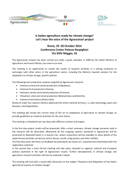
As a consequence of these developments, small farmers are subject to an enormous number
of food safety rules from different sources both as public standards and as private regulations.
Fig. 1 - Private and public food standards
International
Public sector
Food trade
rity
Fo
o
ecu
ds
ds
afe
ty
o
Fo
Private sector
Regional
National
Business
Consumer
Source: Van der Meulen (2011)
Public regulations
Public sanitary regulations have evolved throughout the years through careful management
of the conditions of production/processing/commercialization and the strengthening of judicial
tools associated with the principle of the liability of the agricultural food-chain. Over the past few
years we have witnessed an increase in regulations and norms that force agricultural producers to
follow standard practices that guarantee the production of healthy and safe food.
The regulations put in place by policy makers are:
– of a judicial type, that establish the liability of the producers and sanctions in case of lack of
conformity with regulations or in case of incidents caused by lack of respect for regulations;
– of a procedural type, e.g. the creation of the HACCP procedure or procedures regarding food
traceability;
– concerning the end result, e.g., regulations that set a ceiling on harmful substances that are
permitted in end-products;
– control and inspection (sampling the quality of end-products and inspection of the production and storage of food products).
In order to evaluate sanitary regulations different methods of assessing their impact have been
devised. For example, opportunity cost analysis has helped policy makers in the choice of the
best solution in terms of benefits for society and low total costs, by analyzing different regulatory
options. The economic advantages can be measured, for example, by analyzing the reduction in
resources spent because of food intoxication. Clearly, accounting for all the advantages associated
9
Food safety standards and their impact on the small farms of developed countries
with food sanitary regulations is a daunting task and would require a quantification of the value
of health, the improvement of living conditions and life-span.
Private quality standards
Government regulation on food safety, therefore, is based on the minimum requirements
for market access and mainly related to the obligations of results. Processing and marketing
companies always have a legal responsibility for the consumers’ health problems and are therefore encouraged to adopt insurance schemes in order to protect themselves from the negative
economic impact following the control processes: fines after monitoring and inspections, economic loss from the withdrawal or recall of products, any permanent or temporary suspension of
business by the authorities, brand damage in the view of consumers (Henson and Holt, 2000).
In order to respond adequately to the demands of the community and to improve control of product quality between upstream and downstream sectors, companies have implemented forms of vertical coordination, more or less extensive (in some cases even as far as processes of
real integration).
Some scientific studies have shown that these forms of contract have resulted in changing the balance of power within the supply chain, creating further tensions between the
actors (Giraud-Heraud, Hammoudi, Soler, 2012) and, in some cases, leading to the exclusion
of producers from the system (Fulponi, 2006, Henson and Caswell, 1999).
From a general perspective the reasons why private operators have developed various strategies over the years, are linked to different logics:
– one of them is related to the need for product differentiation with respect to their direct competitors (Caswell et al. 1998; Grunert, 2005; Garella, 2006). This strategy leads companies to
create individual approaches aimed at making the consumer aware, by specific standards (e.g..
system B2C - business to consumer), of the quality checks carried out on production (e.g.
quality controlled by Carrefour, Auchan, ...). Within a context of imperfect market information, an indication of quality to consumers through a system of certification is a method of
differentiation and competitive positioning (Caswell et al. 1998; Grunert, 2005);
– in recent years the B2B (business to business) standards, that are not communicated to consumers, have had a significant growth. These standards refer to a range of behaviors designed
to improve quality and food safety, required by large retailers and processing companies from
their suppliers, and not disclosed to the final consumer (GlobalGap, BRC, IFS, SQF). The
development of this category of collective and voluntary standards requires the presence
of forms of horizontal coordination among groups of enterprises (agri-food and food distribution). These standards, even if voluntary, directly or indirectly affect the conditions of competition and the structure of the chain (Giraud-Heraud et al. 2009, Hammoudi et al. 2009).
3. The role of food standards in international debate
The food alarms of recent years have brought the issue of safety and quality of food to the
center of public debate. For example, with the Beijing Declaration of 2007 on food safety it has
been clearly stated at international level that food safety is an essential public health function
that protects consumers from health risks posed by biological, chemical and physical hazards
in food as well as by the condition of food. Furthermore, many studies (Dupuy, 1979, MaiAnh, 2007; Negri, 2009) have addressed the issue of food security as one of the fundamental human
10
Food safety standards and their impact on the small farms of developed countries
rights. In this context, food security is a fundamental social concern (Tothova, 2009). The same
view is supported by the United Nations. In fact, the International Bill of Human Rights provides the legal framework for the construction of the human right to eat safe food, with observations and interpretations of a general nature prepared by the United Nations Committee on Economic, Social and Cultural Rights. In different contexts, from statements referring to other international legal instruments, the individual right to adequate and safe food has been affirmed in
recent years.
The evolution of food safety legislation as a fundamental human right went, however, in
parallel with the general principle of the development of free trade.
If, on one side, tariff barriers to trade, in accordance with the Uruguay Round, have undergone a significant reduction over the years, on the other, rules of individual countries aimed at
protecting individual health have increased dramatically: many observers feared that these international standards were also used, in some cases, principally as non-tariff barriers. In fact, although
some developing countries have had the ability to adapt to these new challenges, a large number
of them remained excluded from trade with industrialized countries.
In such a context of overall complexity, as evidenced by Josling et al. (2004), in order to
guarantee the freedom of world trade, during the Uruguay Round a central element of the system of multilateral rules for trade in food was the SPS (Sanitary and Phytosanitary) Agreement,
accompanied by the TBT (Technical barriers to Trade) Agreement.
The primary function of the SPS Agreement was to clarify the meaning of Article XX of GATT,
that is the right of countries to protect human health, animals and plants, investigating the issue
of procedures that countries must adopt in order to prevent that generic standards and the precautionary principle can be used improperly to restrict access to domestic markets. The requirements for hazard analysis and critical control points (HACCP - Hazard Analysis and Critical Control Point) and maximum residue limits of pesticides in food and animal feed are some examples
of SPS requirements for market access the EU. Within the WTO (World Trade Organization)
procedures of “notification and review”, have been established such as to enable countries to oppose
those restrictive trade measures that are unsubstantiated from the scientific point of view and, are
therefore, harmful to business. However, the SPS Agreement recognizes the principle that science does not always provide specific answers in terms of potential risks to human health.
The SPS Agreement applies only to those governmental measures that may directly or indirectly affect international trade. If a measure has no trade effect or is imposed by a private firm
or trade association, the SPS Agreement does not apply to it.
The SPS measures include all relevant laws, decrees, regulations, requirements, and procedures and the agreement contemplates that individual members of the WTO may apply SPS
measures on a temporary basis when the scientific evidence on the potential risk is insufficient.
These measures are commonly called “precautionary measures”. Obviously, these areas of discretion for individual countries have led to several trade conflicts (e.g. US against EU for the import
ban on beef derived from U.S. cattle that have been treated with certain growth- promoting
hormones; Japan bans imports of U.S apples on the basis of concerns over the introduction of
fire blight).
However, it is difficult to determine the number of trade conflicts that occur each year, or the
costs of such conflicts. There are widely known conflicts (e.g. meat hormone), but others are literally unknown to the general public (Roberts and Unnevehr, 2003).
Three broad categories of policy instrument can be employed by governments to achieve SPS
protection. Firstly, import bans prohibit the entry of a product entirely. These are most widely
11
Food safety standards and their impact on the small farms of developed countries
applied to products that pose a great risk to human, (or more commonly) plant or animal health.
The second type of SPS measures are technical specifications such as: process, product or packaging standards. Thirdly, information requirements for labelling and checks on voluntary claims
(Roberts et al., 1999).
Attempts to harmonize SPS measures have been made at an international level, even if the SPS
Agreement provides a basis for harmonization of standards starting as a reference with the Codex
Alimentarius and from here to the mutual recognition of national standards, where they can have
demonstrably equivalent results in terms of, protection against food safety risks.
The SPS Agreement also provides for WTO members to facilitate the provision of technical
assistance to other members, especially developing countries. In fact, these specific non-tariff regulations have become a major concern of developing countries regarding access to the international market. Faced with these changes in the international scenario, the attempt to find ad
hoc conciliation with individual countries have been supported worldwide by the use, we could
say abnormal, of regional trade agreements (RTAs) in specific countries.
Regional trade agreements have become an incontrovertible reality in the international trade
scenario. Their number has increased significantly in recent years and there are currently about
200: many of these agreements have been notified to the WTO, but the actual number could
be much higher since some of them have never been reported and many other multilateral
understandings are under negotiation. This results in an increasing share of trade being covered
by regional preferential agreements, and, even more, this situation is becoming no longer the
exception. The effects of regional and bilateral agreements on the multilateral trading system are
still uncertain, as is their impact on trade and sustainable development, but they represent exceptions to the fundamental principle of non-discrimination in the WTO.
Industrialized countries, as well as developing countries, however, have continued bilateral
negotiations, at an even higher speed in recent years, due to the slow progress of the multilateral
trade negotiations of the Doha Round. So while most countries continue formally to declare their
commitment to the successful conclusion of the Doha negotiations, many of them intensify
their efforts in bilateral agreements. This development is widely facilitated by the market access
opportunities provided by bilateral agreements, as in a one to one agreement; non-traditional trade barriers may be included , that is technical barriers to trade and sanitary and phytosanitary measures, with exceptions reserved for specific countries covered by agreements. Obviously,
these agreements create privileged “corridors” in terms of access to the market.
Furthermore, the systems of voluntary private standards of large modern retailing determine
a new form of governance in the food supply chain and some studies show that standards set
by the private sector can help suppliers improve the quality of their products and gain access to
high-quality markets (Swinnen, 2012, Okello, 2012).
4. Food safety standards and implications for farmers in developed countries
It is widely recognized that standards can have a significant impact on trade. A large body of
literature presents debates on the impact of international standards on developing country producers These studies argue that given the widespread poverty in these countries, new norms may
require considerable investment beyond their reach. Other research indicates that many producers have successfully adopted food safety standards that upgrade and enhance their competitiveness worldwide (Swinnen, 2012, Okello, 2012).
12
Food safety standards and their impact on the small farms of developed countries
Furthermore, the standards and the level of border controls influence the direction of trade
flows (Hammoudi, Fakhfakh, Grazia, Merlateau, 2010; Malorgio, Grazia, 2007). Indeed, different types of standard can have distinct trade outcomes. At the same time, many products are subject simultaneously to a range of standards and disentangling the impacts of each is problematic.
Further, the impact of standards is influenced by the strategic manner in which firms respond.
Developing country producers can incur significant costs of compliance whenever changes
are made in international standards or those of their trading partners. Additional costs may also
be incurred in response to new or more stringent requirements of private buyers. These costs can
come in various forms, including fixed investments in adjusting production/processing facilities
and practices, recurrent personnel and management costs to implement the standard and the
public and private sector costs of conformity assessment.
According to Swinnen (2012), food standards create conditions for investment, reduce transaction costs, enforce competition and improve the economic conditions of farmers. The achievement of some standards for some farms in developing countries can be crucial, in the sense that
standards could become catalysts for trade. In fact, the number of producers from developing
countries, that are adopting these quality assurance systems to improve their competitiveness in
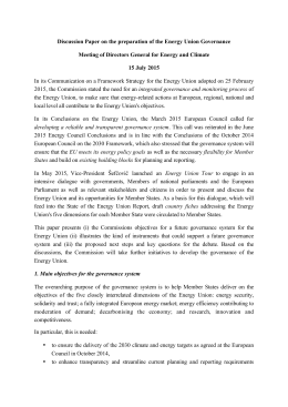
the global market is continually increasing. A demonstration of this effect is that, despite the
proliferation of public and private standards in the EU market, European imports of fruit and
vegetables are continually increasing. In fact, if we analyse specific products such as melons and
watermelons, that have enormous problem of food safety worldwide (with people dying as a
result of salmonella poisoning), in a few years imports from certain developing countries have
enormously increased, despite the evolution of food standards.
Figure 1 - The evolution of imports of melons and watermelons
into the EU-27 2000-2011 (values in US$)
300.000.000
250.000.000
200.000.000
Brasil
150.000.000
Morocco
100.000.000
Costa Rica
50.000.000
0
2000 2001 2002 2003 2004 2005 2006 2007 2008 2009 2010 2011
Source: Comtrade
A first result of this analysis is that public and private standards have no real negative effect
on the export performance of some developing countries. Studies conducted in some developing
nations partially confirm that European imports of such products are more or less equivalent,
with respect to safety risks, to those of European products. However, there remain doubts on
the possibility of fraud for international products. One the other hand, some producers can be
13
Food safety standards and their impact on the small farms of developed countries
integrated into world trade without changing their practices. The imperfections of the control
systems within the EU and their diversity between European countries can lead to opportunistic
and risk-taking behavior by some producers and big importers (Hammoudi et al. 2009). Lacking systematic controls in the production zones and lacking precise certification, the reality of
compliance to sanitary regulations and the investments in the other countries is difficult to quantify. Border control remains the only filter to ensure respect for EU regulation of the imported
products. Few studies have analyzed the effectiveness of border control in the EU. Some descriptive studies (i.e. Fakhfakh et al., 2009) show that heterogeneous rules are applied in different
European ports, which means that some are more rigorous and selective than others in applying
European regulations. Evidently this can lead to fraud with important repercussions on public
wellbeing and on the competiveness of individual firms and producers.
Nevertheless, as shown by Otsuki, Wilson, Sewadeh (2001), small farmers in developing
countries could well have a comparative disadvantage in complying with quality standards
owing to their specific endowments. A critical point associated with the increasing prevalence of
standards is the potential exclusion of developing countries’ small producers from high-standard
export markets, with subsequent negative effects on household incomes and rural poverty. However the evidence in the last few years shows an increasing level of exports from these countries.
According to Chemnitz (2011), farm size is correlated at the margin with the costs of compliance
and the impact of standards on developing countries’ trade flows is, in some circumstances, still
limited. In fact, if evidence from Kenya (Humphrey et al, 2004, Jaffee, 2003), Morocco (Aloui
and Kenny, 2005), Costa Rica (Berdegué et al., 2005) and Senegal (Maertens, 2006) describes
examples of small farmers losing market share as a result of increasing quality standards, other
surveys find very different effects: the inclusion of small farmers in modern value chains can be
found, for example, in Madagascar (Minten, Randrianarison and Swinnen, 2006) and South
Asia (Gulati et al., 2007).
These results show that international literature has been mainly focused on the effects of
standards on developing countries small farmers. As we know, there are very few studies (Romano
et al. 2005) on the effects of the standards on small farmers of developed countries.
Thus many small farms are forced to become certified according to a certain quality standards, because they help them maintain their competitiveness in the marketplace. This point is
confirmed by a direct survey that we have carried out, in Italy in 2012, on more than 25 fruit and
vegetable producers’ organizations (PO), with 10,000 farms associated.
In the survey 94% of these farms had applied private food standards. But the general opinion
of interviewees is that the food standards are the precondition, necessary but not sufficient, for
contracts with large supermarkets. The general crisis seems to have legitimized the market to
consider the fruit and vegetables products a “social safety net”, convenience good, regardless of
the cost required by the production process. Therefore, Italian (and also European) farms negotiate the prices of their products with supermarkets in competition with companies from around
the world who have, in many cases, lower prices and similar standards to European producers in
general. This point is demonstrated by our survey which shows that almost the totality of firms
follow private food standards (such as Globalgap) and of these only 24% sell more than 75%
of their production to large modern retailers, while over 40% sell between 25-50 per cent. The
remaining share of the output of these producers is sold mainly in the wholesale markets in an
undifferentiated way and without receiving a higher price for the food quality standard. Therefore, these products become as commodities in competition with other national non-standardised products and with international products.
14
Food safety standards and their impact on the small farms of developed countries
Figure 2 - Commercialization of products
R>75
24%
R≤25
28%
50<R≤75
5%
25<R≤50
43%
In addition, interviewees indicated some difficulties in achieving these food standards:
– they often do not have a professional quality manager, which creates the need to hire external
consultants;
– in most cases, the documentation is not well understood by the executives of the farms;
– non-homogeneity of standards available, which are often considered too complicated to integrate with each other to meet the needs of multiple buyers.
Therefore, the need to conform with food standards sets a significant administrative and
management burden. These firms also need to invest heavily in drastic changes in terms of production, transport, cold chain, logistics and commercialization. Again, the cost of implementing standards is very important for a firm but its burden may depend on factors exogenous
or endogenous to the firm. The level of compliance costs may increase as a result of the high
number of relationships that upstream producers have with downstream suppliers and then from
the requirement to comply with many, not always equivalent, standards (Fulponi, 2006). Some
studies, moreover, show that the nature of relationships between firms in the supply chain coordinated through a strong and permanent exchange of information, may help reduce the costs
paid by the individual firm (Henson et Humphrey, 2009). The compliance costs investigated are
essentially on private standards and HACCP systems (Romano et al. 2005; Henson et al., 1999,
Semos et al. 2007).
However in a globalized economy, when protection is reduced in domestic markets, and there
are also specific free trade agreements (bilateral agreements) that determine special arrangements
for entrance of food products from specific countries, local products, with high standards of food
safety, would be penalized because they compete with less expensive foreign products and do not
receive a fair return for the compliance costs to achieve standards. In these circumstances domestic producers are penalized compared to their foreign competitors and despite the application
of standards, they need to re-direct their products to less demanding markets, such as wholesale
markets or processing companies.
The answer to this problem would require an international comparison of the level of per-
15
Food safety standards and their impact on the small farms of developed countries
formance of the other countries’ and the European products regarding the more stringent regulations. The problem has, however, received little attention in empirical quantitative studies. Qualitative analysis has been proposed in some studies (Hammoudi, 2010), especially with respect
to productive chains that can represent risks in competitiveness with international products.
Evidently such considerations become more complex when taking into account the difference
between the “dominant” commercial chains of the large buyers (big retailers, traders) that use
private standards and other chains where private standards are not required (wholesale markets,
regional markets and so on, in the developed and developing countries).
5. Conclusion
The last decade has seen notable change in the international scenario for farms and food
firms. The new scenario is, therefore, a renewable policy space with actors, procedures and rules.
Through the 1990s and into the 2000s, international trade in food products expanded significantly, fuelled by changing consumer tastes, advances in production, transport and other supplychain technologies, and the progressive liberalization of traditional barriers to trade. But simultaneously, the increasing prevalence of non-trade measures, such as quality and phytosanitary
standards, is a reality of agri-food trade. A systematic assessment, across countries and across
products, is much warranted, particularly in view of the rising occurrence of trade friction about
food safety and food quality. The private sector is evolving rapidly and in many cases is setting
standards that will supersede public ones.
Taking all these elements of change, this paper has provided a brief overview of the potential
ways in which standards can influence trade from developing countries to developed countries.
The question of the impact of food safety standards (public and private) on the competitiveness
of developed countries’ agriculture is an important topic that refers, for example, to one of the
main axes of the European agricultural model based on the organization of quality in a broad
sense. Behind this approach, there is the question of compatibility between society’s demand for
health and safety in food supply and economic priorities.
References
Aloui O, Kenny L., (2005), The Cost of Compliance with SPS Standards for Moroccan Exports: A Case Study,
The World Bank, Public Disclosure Authorized, 47843.
Berdegué J., Balsevich F., Flores L., Reardon T., (2005), “Central American Supermarkets’ Private Standards
of Quality and Safety in Procurement of Fresh Fruits and Vegetables”, Food Policy, Vol. 30, pages 254-269.
Caswell J.A., Bredahl M.E., Hooker, N.H., (1998), “How quality management metasystems are affecting the
food industry?”, Review of Agricultural Economics 20: 547-557.
Chichilnisky G., (1994), “North-South Trade and the Global Environment”, The American Economic Review,
Vol. 84, No. 4 (Sep.,), pp. 851-874.
Crespi J., Marette S., (2001), “How Should Food Safety Certification Be Financed”, American Journal of
Agricultural Economics, 83, 4: 852-861.
Davis C., (2007), “A Conflict of Institutions? The EU and GATT/WTO Dispute Adjudication”, Princeton
University.
Dupuy R., (1979), Communauté internationale et disparités de développement. Recueil des Cours de
l’Academie de Droit international de La Haye / RCADI.
16
Food safety standards and their impact on the small farms of developed countries
Roberts D., Unnevehr L., (2003), “Resolving Trade Disputes Arising from Trends in Food Safety Regulation:
The Role of the Multilateral Governance Framework” ed. Jean C. Buzby, International Trade and Food
Safety: Economic Theory and Case Studies, USDA, Agricultural Economic Report No. 828
Hammoudi A., Fakhfakh, F., Grazia C., Merlateau M-P. (2010), “Normes sanitaires et phytosanitaires et
question de l’accès des pays de l’Afrique de l’Ouest au marché européen: une étude empirique”, document
de travail, AFD, juillet 2010|100.
Henson S., Caswell J., (1999), “Food safety regulation: an overview of contemporary issues”, Food Policy,
Volume 24, Issue 6, Pages 589-603.
Humphrey J., McCulloch N., Ota M., (2004), “The Impact of European Market Changes on Employment
in the Kenyan Horticulture Sector”, Journal of International Development, Volume 16, Issue 1, pages
63-80.
Fulponi, L. (2006), Private voluntary standards in the food system: the perspective of major food retailers in
OECD countries, Food Policy 31: 1-13
Garella, P. G. (2006), “Innocuous” minimum quality standards, Economics Letters 92: 368-374.
Garcia Martinez, M., A. Fearne, Caswell, J.A. Henson S., (2007), Co-regulation as a possible model for food
safety governance: opportunities for public-private partnerships, Food Policy 32: 299-314.
Giraud-Héraud E., C. Grazia, Hammoudi A. (2007), “Agrifood safety standards, market power and consumer misperceptions”, Journal of Food Products Marketing, Vol. 16-1.
Giraud-Héraud, C. Grazia et A. Hammoudi (2009), “Hétérogénéité internationale des normes de sécurité
sanitaire, stratégie des importateurs et exclusion des producteurs dans les pays en développement”. Cahiers d’ALISS-INRA. www Inra.fr.
Giraud-Héraud E., Hoffman R., Soler L.G.(2012), “Joint private safety standards and vertical relationships
in food retailing” Journal of Economics and Management Strategy, 21.
Grunert, K.G. (2005), Food quality and safety: consumer perception and demand, European Review of Agricultural Economics, 32: 369-391.
Gulati, A., Minot, N., Delgado, C., Bora, S. (2005), “Growth in high-value agriculture in Asia and the emergence of vertical links with farmers”, Paper presented at the workshop “Linking Small-Scale Producers to
Markets: Old and New Challenges”, 15 December 2005, World Bank, Washington D.C..
Hammoudi A., Hoffmann R., Surry Y. (2009), “Food safety standards and agri-food supply chains: an introductory overview”, European Review of Agricultural Economics Vol. 36 (4) pp. 469-478
Henson, S., Caswell, J. (1999), Food safety regulation: an overview of contemporary issues, Food Policy 24:
589-603
Henson, S. et Holt, G. (2000), Exploring incentives for the adoption of safety controls: HACCP implementation in the U.K. dairy sector, Review of Agricultural Economics 22: 407-20.
Henson, S., Brouder, A-M., Mitullah W. (2000), “Food Safety Requirements and Food Exports from Developing Countries: The Case of Fish Exports from Kenya to the European Union”, American Journal of
Agricultural Economics, 82(5): 1159-1169.
Henson S., Loader R. (2001), “Barriers to Agricultural Exports from Developing Countries: The Role of
Sanitary and Phytosanitary Requirements”, World Development Vol. 29, No. 1, pp. 85-102.
Henson S., Blandon, J. (2007), The Impact of Food Safety Standards on an Export-Oriented Supply Chain:
Case of the Horticultural Sector in Guatemala, Nationes Unitads, CEPAL.
Henson, S. et Humphrey, J. (2009), The impacts of private food safety standards on the food chain and on
public standard-setting processes. Joint FAO/WHO Food Standards Programme, Codex Alimentarius
Commission, Thirty-second Session, FAO Headquarters, Rome, 29 June - 4 July 2009. Hikken et Harrison (1999).
Jaffee, S. (2003), From Challenge to Opportunity. Transforming Kenya’s Fresh Vegetable Trade in the Con-
17
Food safety standards and their impact on the small farms of developed countries
text of Emerging Food Safety and Other Standards in Europe. Agriculture and Rural Development Discussion Paper 1. World Bank, Washington D.C..
Josling, T., Roberts D., Order D. (2004), “Food Regulation and Trade: Towards a Safe and Open Global
System”, Institute for International Economics, Washington, D.C. March.
Maertens, M. (2006), “Trade, Food Standards and Poverty: The Case of High-value Vegetable Exports from
Senegal”, Poster paper at the 26th Conference of the International Association of Agricultural Economists,
August 12-18, Gold Coast.
Mai-Anh Ngo, (2007), “La conciliation entre les impératifs de sécurité alimentaire et la liberté du commerce
dans l’accord SPS,” Revue internationale de droit économique, 21, no. 1 27-42.
Malorgio G., Grazia C. (2009), “Strategie produttive e commerciali della sicurezza alimentare: lo standard
GlobalGap e il ruolo delle Organizzazioni di Produttori”, XLIV Convegno SIDEA, Produzioni Agroalimentari tra rintracciabilità e sicurezza: analisi economiche e politiche di intervento Taormina, 8-10 novembre 2007, Milano, FrancoAngeli.
Maertens, M., Swinnen, J. (2006), “Trade, Standards, and Poverty: Evidence from Senegal” LICOS. Centre
for Transition Economics Discussion Papers 177/2006.
Mazzocchi M., Ragona M, Zanoli A. (2013), “A fuzzy multi-criteria approach for the ex-ante impact assessment of food safety policies”, Food Policy 38, 177-189.
McEachern MG, Warnaby G., (2004), Retail ‘Quality Assurance’ Labels as a Strategic Marketing Communication Mechanism for Fresh Meat, The International Review of Retail, Distribution and Consumer Research,
Volume 14, issue 2.
Minten, B., Randrianarison, L., Swinnen, J. F. M., (2006), “Global Retail Chains, International Trade and
Developing Country Farmers - Evidence from Madagascar”, Contributed paper at the IATRC Summer
Symposium 2006, “Food Regulation and Trade: Institutional Framework, Concepts of Analysis and
Empirical Evidence”. May 28-30 2006, Bonn.
Mitchell, L., (2003), “Economic Theory and Conceptual Relationships Between Food Safety and International Trade”, Cap. 2 in Buzby, J.C. (ed.) “International trade and food safety: Economic theory and case
studies” USDA/ERS Agricultural Economic Report 828, November.
Moenius, J. (1999), “Information versus Product Adaptation: the role of Standards in Trade” Working paper,
University of California, San Diego.
Negri, S. (2009), ”Global Health Governance”, volume, n. 1 (fall 2009) http://www.ghgj.org.
Okello, JJ (2012), “Compliance with International Food Standards: effects on family farmers”, AfD-INRA
Conference on “Food Safety, Trade and Development”, Paris Dec 2012.
Otsuki, T, Wilson, J. Sewadeh M., (2001), “Saving two in a billion: quantifying the trade effect of European
food safety standards on African exports”, Food Policy 26, 495-514.
Romano D., Cavicchi A., Rocchi B. et G. Stefani (2005), Exploring costs and benefits of compliance with
HACCP regulation in the European meat and dairy sectors, Act Agriculture Scand Section C, 2005; 2:
52-59.
Semos A. et A. Kontogeorgos (2007), “HACCP implementation in northern Greece: food companies’ perception of costs and benefits”, British Food Journal, 109, 5-19.
Swinnen, J., (2012) “Food Safety, Trade and Development - Linking Rich Consumers to Poor Producers”,
AfD-INRA Conference on “Food Safety, Trade and Development”, Paris Dec 2012.
Tothova, M. (2009), The Trade and Trade Policy Implications of Different Policy Responses to Societal
Concerns, OECD Food, Agriculture and Fisheries Working Papers, No. 16, OECD, Paris.
Unnevehr L., Roberts D. (2002), “Food safety incentives in a changing world food system”, Journal of Food
Control 13: 73-76
Unnevehr, L. and Roberts D. (2005), “Resolving Trade Disputes Arising from Trends in Food Safety Regula-
18
Food safety standards and their impact on the small farms of developed countries
tion: The Role of the Mulitlateral Governance Framework” World Trade Review, 4 (3): 469-497.
Van der Meulen B. (2011), Private food law - Governing food chains through contract law, self-regulation,
private standards, audits and certification schemes, Wageningen Academic Publishers.
19
Vuota
PAGRI 4/2012
Improving Measures for Targeting
Agri-Environmental Payments: The
Case of High Nature Value Farming
JEL classification: Q18, Q56, Q57.
Irina Solovyeva*, Ernst-August Nuppenau*
Abstract. The debate on optimization of policies and instruments for European agriculture has
lasted for several decades and there is still no consensus about it. Although there is unanimity on the targets these policies should achieve, there is an on-going
discussion about policy tools for the practical implementation of the CAP as regards agri-environmental
payments. The aim of this paper is to contribute to
this discussion by looking at the approaches developed
to evaluate environmental and economic efficiency
simultaneously, as well as to examine possibilities for
more targeted agricultural support by implementa-
tion of economic-environmental efficiency analysis.
In this regard it is especially interesting to consider
the case of support for sustainable land use practices
such as in HNV (high nature value) farming and
the opportunities for implementing such analyses in
areas of HNV agriculture: we consider in particular disadvantaged mountain areas in the Romanian
Carpathians and the bordering areas in the Ukrainian Carpathians.
Keywords: CAP measures, agri-environmental
payments, economic-environmental efficiency, HNV
farming.
1. Introduction
The debate on optimization of policies and instruments for the European Agriculture Policy
(CAP) with regard to environmental aspects has lasted for several decades and there is still no
consensus of opinion on it. There is certainly unanimity on the targets these policies should
achieve such as: (1) they should be formulated in order to obtain economic efficiency together
with the simultaneous achievement of environmental goals and (2) they should recognize regionally specific aspects and subsidiarity. However, since the early 1990s, when agri-environmental
issues were first reflected in the CAP, there has been an on-going discussion on policy tools for
the practical implementation of CAP targets and on those instruments which should particularly
serve as a basis for agri-environmental payments. The range of opinions on suitable policies is
quite wide. Generally it seems that the currently existing system of agri-environmental payments
and the cross-compliance mechanism is justified and positively evaluated only because there are
no alternatives (Cooper et al., 2009; FAO, 2010).
However many researchers have criticized the implementation of the CAP system for inef-
* Department of Agricultural and Environmental Policy, Institute for Agricultural Policy and Market Research, Justus-Liebig University,
Giessen, Germany.
21
Improving measures for targeting agri-environmental payments: the case of high nature value farming
ficiency and inconsistencies noticeable between policy measures and objectives (Arovuori, 2008;
Mann, 2005). Some specifically argue that there is an obvious contradiction in the current CAP
policy: on the one hand, there are agri-environmental payment schemes offering support to sustainable land use practices; on the other hand, there are market and income support payments
which give incentives to intensify agricultural production (Pacini et al., 2004). In any case there
is a constant search for a suitable policy scheme which could replace the existing system of payments and which would consider a more targeted distribution of payments.
It is especially interesting to consider the case of support for sustainable land-use practices
such as in HNV (high nature value) farming which is recognized in some parts as the CAP and
as a set of farming practices which are successful in providing positive externalities and environmental services. Those member states, which acknowledge and support the HNV farming concept and maintain HNV agriculture, sustain it mainly through Rural Development Programmes
(RDPs) (Beaufoy, 2007).
The aim of this paper is to contribute to the above-mentioned discussion on EU agricultural
policy schemes by looking at the approaches developed to consider ecological and economic
efficiency simultaneously and to examine the question of the possibilities of measuring economic
performance in agriculture by considering environmental efficiency. To do that, we give a review
of the existing literature on economic-environmental efficiency and on incorporation of environmental externalities into analysis of production efficiency. Moreover, in the paper, we reflect
on opportunities of implementing such analyses in areas of HNV agriculture: we consider, in
particular, disadvantaged mountain areas in the Romanian Carpathians as target areas. Bordering areas in the Ukrainian Carpathians were also taken as a region for comparison because they
have generally similar conditions but the efficiency analysis can be conducted with the exclusion
of the influence of the EU agri-environmental payments (which have already been introduced
in Romania). This article brings into the discussion the question of addressing efficient provision of nature if there are possibilities for more targeted agricultural support in the case of HNV
farming.
The paper is structured as follows: after the introduction, the theoretical background on
policy intervention, specifically in agriculture, is presented, and subsequently the main policy instruments, their mixes, and their possible problems are considered. The third part deals
with the CAP itself. First, its development, and, after that, the current state and possible future
amendments are described with special consideration of agri-environmental schemes; finally, the
most debated problems and inconsistencies of the CAP are mentioned. In the fourth part we
give an overview on the options for solving some of the problems mentioned: some approaches
for evaluation of farms’ performances which are mentioned in the literature are considered, and
then an alternative approach for performance analysis is discussed which considers economic
and environmental parameters simultaneously within efficiency analysis; this part shows how the
methodology was developed and used in various studies and deals with the positive sides as well
as the limitations of the approach presented. The fifth part considers the special case of HNV
farming support and reflects on implications of the efficiency evaluation approach described for
the special HNV farming areas at the research sites in the Romanian and the Ukrainian Carpathians. The conclusion sums up the discussion presented in the paper on the possible solutions to
more targeted support within the CAP.
22
Improving measures for targeting agri-environmental payments: the case of high nature value farming
2. Agri-environmental policy: theoretical background
The aim of this part is to give an overview of the theoretical foundation for agri-environmental policies and discuss the most important justifications for policy interventions in agriculture within a market economy. Two dimensions will be mentioned: the environmental and the
economic perspectives. The same dimensions will be considered subsequently in other parts to
analyse the methods of performance evaluation or the policy mechanisms. The subsection concerning the political perspective deals with main components of policy design: the objectives of
the agri-environmental policies as well as policy instruments and their mixes.
2.1. Environmental perspective
A central aspect of agri-environmental policy is the recognition of the various impacts of
agricultural practice on material flows of pollutants, nature biodiversity, landscapes, etc. Tillage practices, usage of chemical substances for fertilization, pest control, water consumption,
etc. can significantly influence nature and its components. In particular, intensified agricultural
production can lead to serious environmental problems such as soil erosion, degradation of
water quality, reduction of wild life habitats, etc. (Bonnieux et al., 2006). Production systems
and practices differ in the impacts they have on the environment, which can be positive or
negative (for example, the differences between the production approaches in organic and in
conventional farming).
To justify policy intervention from the perspective of the environment, it has been important
to realize that changes in farming practices towards nature-friendly techniques can have a strong
positive influence and solve some serious environmental problems. Some forms of agricultural
management can provide better environment; for instance, such characteristics as agricultural
land use, the size and structure of the farm, agricultural infrastructure, etc. can influence, to a certain extent, types of positive or negative environmental change (Cooper et al., 2009). This aspect
has increased the importance of the role farm practices play in managing environmental impacts:
farmers are not only food suppliers but also the “conservers of the landscape” and “protectors of
natural resources” (Pacini et al., 2004).
2.2. Economic perspective
The economic perspective of policy intervention, in this case, deals with two main terms:
environmental externalities and public goods. The impacts of agricultural production on nature
influence not only the producer but also other members of society, causing additional costs (in
the case of negative external effects) or benefits (positive external effects). The concept of public
goods implies that certain goods are characterized by non-rivalry and non-excludability (Schader,
2009) and these public goods can be provided by farming practices which are environmentally
friendly only if governance is clear.
Both externalities and public good aspects are considered as market failures, since external
effects create costs which are not compensated or benefits which are not paid and environmental
public goods can be undersupplied since the provider has no incentives to provide it without
compensation (Cooper et al., 2009). This justifies policy intervention in the market mechanism
and provides an important framework for agri-environmental policies the aim of which is usually
to internalise the external effects.
23
Improving measures for targeting agri-environmental payments: the case of high nature value farming
2.3. Policy perspective
Agricultural policy is an example of multi-objective policy. Most of the aims of current agricultural policy can be accommodated into a sustainability concept (FAO, 2010) and the particular sustainability of farming also implies multiple objectives (Pacini, 2003). Although the term
itself is quite ambiguous, we can argue that sustainability in agriculture includes two important
components: socio-economic and bio-ecologic or environmental dimensions (De Koeijer et al.,
2002). The main policy objectives should cover these dimensions and include such aims as securing farmers’ incomes, allowing increase in productivity, recognizing structural developments,
market stabilization, reasonable consumer prices, availability of supplies and of course environmental concerns (Arovuori, 2008), which are, in their turn, comprised of further specified targets
that will be discussed in part 3 of this paper.
There is a wide variety of policy instruments which can be used to achieve the above- mentioned
objectives. The overview of these instruments is given in Table 1 (based on Schader, 2009).
Tab. 1 - Overview of the instruments in agri-environmental policy
Instrument
Standard regulation
Short description
Standard regulation bans the use of certain (detrimental) inputs and prescribes the
use of precautionary measures
Environmental tax
Input-oriented taxes allow farmers to use the taxed input only in case it can still
be profitable with the tax. There may be also output-oriented taxes (e.g. undesired
output)
Tradable quotas
Contrary to the environmental tax which deals with price regulation, the quotas
regulate the quantity of environmental certificates tradable on the special market
Environmental auctions
An effective solution on a smaller scale
Communicative policies
Communicative policies lead to higher uptake levels of the agri-environmental
schemes on the production side and improved market transparency on the side of
the consumer
Agri-environmental
schemes and measures
AE schemes represent a voluntary instrument and are a mixture of regulatory
instruments with economic incentives; compensate farmers for yield and income
loss and higher production costs due to implementation of environmentallyfriendly practices
Cross-compliance
Cross-compliance rules represent an obligatory approach. Non-compliance to
certain environmental standards makes farmers ineligible to receive other types of
payments, for instance direct payments
Community-based
schemes
The idea behind this instrument is to fund local initiatives aimed at pursuing policy
goals at regional or local level
Source: based on Schader, 2009
Beside these instruments a certain number of other tools are connected directly to the economic dimension, which implies the use of several instruments for one policy. This diversity of
instruments causes major difficulties for policy design presenting the task of combining policy
tools in the most favourable i.e. effective way, in order to create the needed incentives to farmers
for the provision of environmental public goods. There are some rules for effective policy measures and policy design (OECD, 2007):
• Good understanding of the (environmental) problem which should be addressed;
• “Cost-benefit” criterion – the marginal cost of implementing the mix of instruments should
be less than the marginal benefit;
24
Improving measures for targeting agri-environmental payments: the case of high nature value farming
• “Cost-effectiveness” criterion – the marginal cost of applying the mix of instruments should
be as low as possible;
• “Environmental effectiveness” criterion – the marginal environmental benefit from implementation should be as high as possible;
• In particular the question of the optimal number of instruments in policy design is usually addressed from the perspective of the Tinbergen rule (Tinbergen, 1966), which implies
that each instrument within one policy should address one specific policy objective, i.e. the
number of tools used should be equal to the number of policy aims.
Following these rules, we can sum up other important aspects which are crucial for effective
agri-environmental policy:
• Thorough analysis of the problem is necessary, the focus of the policy is on efficiency;
• Sufficient information on socio-economic and environmental parameters is needed;
• It is essential to develop economic evaluation techniques to measure the effectiveness of
policy measures, to estimate the costs or benefits of certain farming types and to evaluate
the performance rates of certain farms with regard to the provision of environmental public
goods. The latter has implications for more accurate targeting of agri-environmental policy
measures which plays an important role and will be partially addressed in the following sections of this paper.
3. The CAP as a mix of instruments for agri-environmental policy
3.1. Development, current implementation and future of the CAP
The history of the CAP (European Common Agricultural Policy) starts in 1957 and it has
been constantly subject to new developments. Based on the Treaty of Rome, it introduced various market measures with the main objectives of increasing agricultural productivity and providing income support to European farmers (Cooper et al., 2009). Although certain measures of
agri-environmental policy were already implemented in some European countries in the 1980s,
the first introduction of environmental concerns into the CAP framework took place in the
mid-1990s when McSharry reforms were started (FAO, 2010). The EU Regulation 2082/92
covered such impacts as water quality, soil quality, biodiversity, and landscapes (European Commission, 1998). The relevant measures were classified into 3 groups: environmentally-beneficial
in productive farming (including input reduction, organic farming, extensification of livestock,
etc.); tools for non-productive land management (including maintenance of the countryside and
landscape features, set-aside, etc.); and socio-economic measures (including training and education) (European Commission, 1998).
Next, changes within the CAP were introduced within the period of the Agenda 2000 – the
policy developments for the 2000-2006 period – and with the 2003 reform. Within this period
such measures as cross-compliance and decoupling of direct payments from production were
introduced. This was implemented through the Single Payment Scheme (SPS) which is paid per
hectare of land and does not depend on agricultural output. Cross-compliance implies that SPS
is paid as long as the land is kept in Good Agricultural and Environmental Condition (GAEC)
(FAO, 2010; Brady, 2011). There have been many explanations for the choice of policy (Bartolini et al., 2012); a popular explanation is the theory of compromise and doing things at the minimum as well as having a focus on financial flows rather than on real concern for the environment.
The same strategy was followed in the CAP framework for the 2007-2013 period, which
25
Improving measures for targeting agri-environmental payments: the case of high nature value farming
was formed around two pillars, with Pillar 1 representing traditional commodity orientation
including decoupled direct payments as well as cross-compliance, and Pillar 2 containing rural
development programmes (RDPs) (FAO, 2010). Three Axes of the Pillar 2 cover all dimensions
of sustainability: Axis 1 deals with economic issues, Axis 2 focuses on environmental and land
management issues with agri-environmental measures as a part of it and Axis 3 considers social
and rural community issues (FAO, 2010).
Concerning an assessment of the policy, Cooper et al. (2009) put into the focus of their study
10 environmental public goods provided by agriculture which are under the influence of the
CAP. These include agricultural landscapes, farmland biodiversity, water quality, water availability, soil functionality, climate stability with relation to carbon storage and measures to regulate
green house gas emissions, air quality, resilience to flooding, resilience to fire. These authors
also divide the current CAP measures into three groups (Cooper et al., 2009): measures which
are focused directly on the provision of environmental public goods (like agri-environmental
schemes); measures with partial focus on the environmental issues (for example, support of LFA
– less favoured areas); measures with no direct focus on environment but with potential to have
a positive influence on nature (decoupled direct payments and cross-compliance). These interdependencies determine the complex structure of the CAP instrument mixes where each instrument may be used to reach several objectives.
All measures for the next CAP reform for the period of 2014–2020 are still under discussion. However it is already clear that there are some serious challenges for agricultural policy in
Europe:
• The CAP reform is developing in the framework of Europe 2020 Strategy of “smart, sustainable and inclusive growth” which, among other issues, includes “the promotion of a more
resource-efficient, greener and more competitive economy” (FAO, 2010). This implies that
the CAP will keep a strong focus on the environmental aspects of agriculture. Moreover
the current discussion about percentages of area to be devoted to ecological main structures
by farmers, such as 7% of arable land for fallowing, crop rotations, etc., and the intensive
discussion about what is eligible to be considered as a greening measure, show the will and
need to proceed in the direction of getting better results out of a new CAP in terms of nature
conservation;
• The problem of limited financial resources will pose additional challenges for all the actors
and will require two important special measures within the policy design:
– Improved justification of agricultural support as a definite benefit for society and
– Improved cost-effectiveness of agri-environmental policies.
The latter issue belongs to the most debated problems of the agri-environmental aspects of
the CAP and is discussed among other issues in the next subsections of this paper.
3.2. Problems and trade-offs of the CAP
As we have already mentioned, the effectiveness of the CAP can be questioned from the perspective of the Tinbergen Rule which implies that one policy instrument is needed for one policy
objective to create an efficient policy. In the sub-section 3.1 we have mentioned the complexity
of instrument mixes within the CAP which means that it fails to comply with the Tinbergen Rule
(Arovouri, 2008). However this rule was formulated under certain assumptions which should be
emphasized: there should be no conflicting goals or co-benefits of policies and there should be
no transaction costs (Schader, 2009). This is hardly applicable to agri-environmental policy in
general and to the CAP in particular due to the complex system of interdependencies of various
26
Improving measures for targeting agri-environmental payments: the case of high nature value farming
tools. For example Schader (2009) shows that multi-objective policy should not be excluded on
the basis of the Tinbergen Rule only. Rather, he shows, in his study of organic farming, that it
is not the only criterion for the cost-effectiveness of a policy: the effectiveness of organic farming
has to be regarded as a single instrument for several objectives. It was proved to be comparable to
the option of combined agri-environmental measures (Schader, 2009).
A lot of criticism has been directed against the decoupling and cross-compliance policies. For
instance, it was argued that decoupling would lead to a reduction of agricultural activities and
production, especially in marginal rural areas (Brady, 2011). The SPS (Single Payment Scheme)
is seriously criticized as an inappropriate measure for providing environmental stewardship for
rural landscapes and as an inefficient environmental policy, at least as regards landscape values
(Brady, 2011). The ability of the cross-compliance framework to avoid all the negative environmental consequences of decoupling is also questioned: the argument is that “commercial constraints will necessarily dominate” and environmental public goods will be undersupplied (Beard
and Swinbank, 2001). Payments within this policy measure stay on the same level and are not
connected to the levels of nature provision: if some farms show better environmental indicators
than others, they still receive the area-based payment. Agri-environmental schemes and payments
are yet to be developed to solve this problem. They face another challenge however: since the
compensation level is not adapted to real performance of farms, this leads to overcompensation
of some producers (Schader, 2009). Sensible methods for evaluation of farm performance are
needed for more targeted and balanced agricultural support.
These contradictions which underlie the current CAP measures are a problem and a matter of
conflict between environmental measures and other measures for support of agricultural production: although the agri-environmental issues are recognized and accommodated into the current
policy, the main objective of the CAP is to increase agricultural productivity. Aims may contradict each other. The question is: if there is a certain farming system or a set of farming practices
within a region which is able to reach both aims simultaneously in the most efficient way, how
can we incorporate into policy the incentive to follow the best practice example?
The problem of performance evaluation of farms and ways to targeting of agri-environmental
support will be addressed in the following parts.
4. Considering economic and environmental efficiency within the CAP
4.1. Evaluation approaches to support the CAP: an overview of the literature
As mentioned above, the agri-environmental policy itself and agri-environmental schemes in
particular face a lot of challenges since it is very complicated to measure environmental effects in
practice and to evaluate how effective the policy measures are. Many approaches are developed
in the literature for solving the issue of evaluation. In this paper we consider a few evaluation
approaches which do not cover all the scope of existing methods but give an idea of how this
assessment can be performed. These methods contain the following common features:
• They are farm system approaches to evaluation (with the exception of the case presented by
Schader (2009) where a sector-based approach was applied);
• They include modelling of economic and environmental effects;
• The main aim of these methods is to evaluate measures of agri-environmental policy.
For example, Schader (2009) used a cost-effectiveness approach for the evaluation of the
Swiss agri-environmental policy, in particular of organic farming support. The approach used
27
Improving measures for targeting agri-environmental payments: the case of high nature value farming
linear programming (LP) and modelled farm management and relations between farm internal
activities as well as farmers’ responses to changes in exogenous conditions in the form of direct
payments or product prices; it also compared farm groups (organic and non-organic farms) within the sector and took into account policy uptake, environmental effects and public expenditure
for agri-environmental policy, notably as determinants for cost-effectiveness (Schader, 2009).
Although only three environmental effects were considered (fossil energy use, biodiversity and
eutrophication with nitrogen and phosphorus), the analysis (with the use of this model) presented interesting results considering cost-effectiveness of organic farming support and showed
differences between organic and conventional farms. It proved that generally organic farms perform better with respect to the environmental impact. Moreover it showed that organic farming
support as a multi-objective policy provided individual environmental effects at a higher (but
comparable cost) than specialised targeted agri-environmental measures.
In their approach Falconer and Hodge (2001) used the “production ecology methodology”
to see how different measures of pesticide use control influence farm performance (Falconer
and Hodge, 2001). The idea behind this approach is to analyse simultaneously production of
agricultural outputs and environmental externalities. It resulted in connecting economic farm
modelling with ecological models developed to evaluate environmental consequences of pesticide
use. Economic performance models were developed for two farm groups: commercial crop production and “progressive” farming which included commercial as well as reduced input practices.
The environmental model aggregated “hazard indicators for pesticides” which were identified
for nine ecological and human-health dimensions scored according to labelled warnings (Falconer and Hodge, 2001). The two models were combined into a farm resource allocation model
including both the economic components and indicators for environmental hazards. Finally a
two-dimensional frontier analysis was used to see the differences between the outcomes of the
various policy instruments applied. The approach also uses an LP model.
The model developed by Pacini et al. (2004) aimed at comparing the economic-environmental performance of organic and conventional farms under various policy scenarios, and at
measuring the superiority of organic systems for various amenities. Versions of integrated ecological-economic LP models for organic and conventional farming systems were used to compare various aspects of their performance: technical, environmental and economic. In principle,
the model used input-output matrices which were extended to include emissions and various
indicators from ecological models such as nitrogen leaching, soil erosion, ground and surface
water balances, herbaceous plant biodiversity, and others (Pacini et al., 2004). The combination
of these models allowed the evaluation of the production costs of environmental externalities
provided by organic methods. The modelling framework is described as indicating efficient use
of measures for the policy with multiple objectives because “it is based on actual environmental performances, it takes into account site-specific pedo-climatic factors; and it is holistically
designed and considers trade-offs between potentially conflicting environmental goals” (Pacini
et al., 2004).
To sum up, it is necessary to mention that the approaches considered were developed to
evaluate and compare the performance of various farming systems with respect to economic output and environmental impacts. However the main aim of these methods is to evaluate various
agri-environmental policies. Another limitation is that most of them consider only a few environmental effects. Within the scope of this paper we are more interested in how to distinguish
farmers according to their economic-environmental performance within a certain farming system. In order to make the agri-environmental support more targeted, we think that it is necessary
28
Improving measures for targeting agri-environmental payments: the case of high nature value farming
to consider farm performance. Admittedly, the approaches described can be applied to this kind
of assessment; however the next subsection will deal with a further method for evaluation which
offers new perspectives for policy analysis and design.
4.2. Opportunities for efficiency evaluation
With regard to the trade-off between the two most significant objectives of the CAP which
are often contradicting one another (i.e. the increase in productivity and the provision of environmental goods) it is important to take into consideration evaluation methods which would be
able to provide an analysis combining both aims. Efficiency evaluation which would consider
economic and environmental performance seems to be a suitable solution. This subsection gives
an overview of the methodological developments in this area and discusses the possible implications for the CAP.
The measurement of production efficiency is usually based on physical and monetary inputs
and outputs. The traditional setting of production economics (see Figure 1) implies that “a firm
consumes inputs (e.g., labor capital, materials, energy) to produce economic outputs (i.e., goods
and services)” (Kuosmanen and Kortelainen, 2004). Technical efficiency of this firm implies that
its input-output combination lies on the boundary of the set of all possible inputs and outputs
which represents technology (Kuosmanen and Kortelainen, 2004). A commonly used measure
of efficiency is a ratio in the form of:
Output
Efficiency = ––––––––––
Input
Although many other measures (such as, for instance, relative efficiency) are used (Cooper et
al., 2002, Bousofiane et al., 1991), it lies at the core.
Fig. 1 - The traditional setting of production analysis
Inputs (x)
Outputs (y)
Firm
Source: Kuosmanen and Kortelainen, 2004.
It is important to point out that an incorporation of environmental externalities into efficiency analysis provides a more complete representation of production technology. At the same time
the omission of environmental effects may create biases in evaluation of production techniques
and underestimation of the environmentally friendly technologies (Sipiläinen et al., 2008). The
methodological challenge of this approach is the consideration of how these externalities can be
incorporated into the efficiency model: as an input or as an output.
A number of research papers elaborate on consideration of environmental impacts of production in efficiency analysis. The majority of them deal with negative externalities. Some authors
29
Improving measures for targeting agri-environmental payments: the case of high nature value farming
assume that negative environmental impacts are technically outputs and therefore argue that
environmental externalities should be modelled as an undesirable output (Färe and Grosskopf,
2004). Another group of researchers sees it as a conventional input; they justify this, for instance,
by the fact that undesirable environmental effects as well as inputs incur costs to the firm (Kuosmanen and Kortelainen, 2004; Lauwers and Van Huylenbroeck, 2003; Reinhard et al., 1999, De
Koeijer et al., 2002). However there are also attempts to model positive externalities which are
considered as non-marketed output or as desirable by-products (Sipiläinen et al., 2008).
The notion of environmental efficiency provides many possibilities for economic evaluation
of environmental impacts. However, modelling approaches differ. Usually environmental efficiency is defined either as “the ratio of minimum feasible to observed use of an environmentally
detrimental input” (Reinhard et al., 1999) or as the ratio of economic value added to environmental pressures (Kuosmanen and Kortelainen, 2004).
Methods of evaluation in case of environmental efficiency also vary. For instance, Reinhard
et al. (1999) use an econometric approach to estimate the environmental efficiency of nitrogen
surplus in agriculture. The same group of authors used the SFA approach (Stochastic Frontier
Analysis) to assess the same parameter with consideration of multiple environmentally detrimental inputs (Reinhard et al., 2000). But the method which we would like to consider in this
paper and which is also often used for this type of analysis, is the DEA method (Data Envelopment Analysis).
DEA is an approach for comparing efficiency of various organizational units (farms) with
multi-input and multi-output production options (Sipliläinen, 2008). Efficiency is calculated
for a relatively homogenous set of decision making units (DMUs). DEA constructs the efficiency frontier (the most efficient combinations of inputs and outputs performed by some of
the DMUs in the set) and calculates the distance to this frontier for the DMUs which are not
situated at the frontier and therefore are less efficient (De Koeijer et al., 2002). “DEA does
not require the user to prescribe weights to be attached to each input and output... and it also
does not require prescribing the functional forms” (Cooper et al., 2002). So minimal prior
assumptions are made and the approach lets the data “speak for themselves” (Kuosmanen and
Kortelainen, 2004). This is especially beneficial for the case of environmental evaluation since
subjective assessment of weights for the aggregate level of environmental impacts is quite a challenging procedure (Kuosmanen and Kortelainen, 2005). Moreover DEA uses LP models which
are solved for every DMU.
DEA has also been used for agricultural policy evaluations. For example, De Koeijer et al.
(2002) applied DEA to estimate technical and environmental efficiency of Dutch sugar beet
growers. The environmental efficiency in this analysis is based on the environmental impacts of
polluting inputs (pesticides and nitrogen application). Reinhard et al. (2000) considered the use
of multiple environmentally detrimental inputs (excess nitrogen and excess phosphate use and
total energy use) within the DEA approach to evaluate the environmental efficiency of Dutch
dairy farms. In contrast to the approaches mentioned Sipiläinen et al. (2008) used the DEA
method for efficiency evaluation with positive externalities: they compared the performance of
organic and conventional farms modelling the existence of two outputs – conventional output
(crop yield) and environmental by-product (agricultural biodiversity). The latter research shows
that the method can be used to evaluate the performance of a holistic farming system such as in
this case, organic farming.
Considering these attempts to evaluate performance at farm level, we can argue that DEA is
a suitable method for measuring the efficiency of farm performance considering environmental
30
Improving measures for targeting agri-environmental payments: the case of high nature value farming
impacts. On the one hand it allows consideration of multiple environmental effects (Reinhard
et al., 2000) and on the other, it also provides an opportunity of modelling positive as well as
negative externalities (in the form of outputs and inputs respectively). In addition, DEA results
can be used practically in many other ways, for instance, to ascertain how the DMUs can become
more efficient, to form peer groups, to identify efficient operating practices and strategies, to
allocate resources, etc. (Bousofiane et al., 1991). The aim is now to use DEA for evaluation of
farm performance.
Despite all the positive features, it is obvious that the approach also has some limitations.
DEA is based on certain assumptions such as availability of resources, convexity and absence of
statistical errors in the data set. In fact “the extensive data requirement” is usually mentioned as
the main limitation of this method (Kuosmanen and Kortelainen, 2005). Since the efficiency
frontier is built simultaneously and no prior assumptions are made, the data should be accurate
and reliable. It is also important to point out that data availability, especially for analysis with
consideration of environmental impacts of policy (payments), is a major problem for all evaluation methods including those described in subsection 4.1. At the same time the information
requirement is very important for policy design: “The omission of information on many environmental aspects may lead to misjudgements in the objective policy-making process and conflicts
between different government programmes or regulations” (Pacini, 2003). Another problem
within DEA, which should be mentioned, is connected to the simultaneous evaluation of multiple positive and negative environmental impacts. First, a clear framework should be elaborated
which accommodates the environmental effects and groups them into two categories according
to their positive or negative impact. It should also be decided how these impacts are defined – as
inputs or as outputs. Secondly, the interdependencies between the environmental effects should
also be considered (Kuosmanen and Kortelainen, 2005).
The next part of this paper considers the special case of HNV (High Nature Value) farming
and the possible implications of the efficiency evaluation approach described for HNV areas.
5. Efficiency evaluation in the case of HNV farming
5.1. HNV farming within the CAP
The concept of HNV (High Nature Value) farming is rather new (Beaufoy et al., 1994;
Beaufoy, 2007, Andersen et al., 2003), though it covers well-established conceptual approaches
in farming system and landscape analysis (such as extensive farming, farming with nature provision). The concept was developed for different landscapes, within which nature is still found
intact and ecological values are ranked high (Fig. 2). HNV farming applies to situations in which
nature co-exists and coincides with farming activities as well as in situations where farming is
supportive of greater biodiversity in semi-natural landscapes. The purpose of this concept is to
compare and contrast extensive farming systems to farming systems that do not care for nature
or even degrade nature. The aim is to link the three components, ecology, farming, and public
policies, in such a way that they get “equal” recognition in management concepts. Since most
of the payments within the CAP framework were intended for Europe’s most productive and
competitive farmers, HNV farming is an attempt to identify and define alternative types of farming that also need public support but, on the other hand, deliver increasingly scarce ecosystem
services at both local and EU levels. The central objective is to shift public support in favour of
low intensity farming across extensive areas of landscape (Beaufoy, 2007).
31
Improving measures for targeting agri-environmental payments: the case of high nature value farming
Fig. 2 - Characteristics of HNV farming
Low-intensity management
Livestock
Nitrogen
Biocides
HNV
Type 1
% of semi-natural land cover
Grass, scrub
Trees
Field margins
Source: Beaufoy, 2007,
Type 2
Diversity of land cover
Crops
Fallows
Grass, scrub
Trees
Water bodies
As we can see, the concept of HNV farming is based, first of all, on the idea of low-intensity
farming and more importantly on the concept of a holistic system of extensive land use practices
which includes the notion of connectivity between farming and nature. Therefore HNV agriculture provides the public good of biodiversity conservation as well as other environmental amenities and facilitates an improvement in the ecosystem, possibly at lower cost than single measures.
In contrast to other farming systems, in this case the main policy task is not to encourage the
farmers to produce in a more environmentally friendly manner since the basic assumption of
HNV is that nature provision is already a part of this agricultural system. This type of farming
is based on traditional knowledge and local culture. However there are other important challenges for such policy: intensification or abandonment should be necessarily addressed and agrienvironmental schemes should be adopted. Since these farming systems dominate in marginal
and remote (usually mountainous) areas (Baldock et al., 1996), abandonment, which is related to
inability to adapt land management to social and economic pressures (MacDonald et al., 2000),
is a significant threat. The main impacts of this trend on the environment are usually connected
directly to biodiversity losses, changes in the landscape mosaic and soil depletion (MacDonald et
al., 2000). An assumption is that HNV farming, as a holistic sustainable agricultural system, can
provide a solution for these challenges; therefore all kinds of support measures can be regarded
as environmental measures.
Currently HNV farming is supported through Pillar 2 of the CAP and RDPs (Beaufoy,
2007). The main measures within the CAP which have an impact on this type of farming are
for instance: i) natural handicap payments or aid to farmers in less favourable areas (measures
211 and 212), ii) Natura 2000 programme for special conservation zones (measure 213), iii)
agri-environmental schemes (measure 214), and iv) partially also payments for conservation and
upgrading of the rural heritage (measure 323) (Cooper et al., 2009).
Summing up, we should emphasize that HNV farming can be regarded as a holistic system which comprises extensive farming practices favourable to the environment. In contrast
to organic agriculture, which can also be distinguished through its special approach to production techniques, this system is, moreover, incorporated into the way of life of local people and
32
Improving measures for targeting agri-environmental payments: the case of high nature value farming
strongly connected to the local culture and traditional knowledge. However, we argue that even
within the homogenous group of HNV farms there can be differences in performance and in
environmental provision which it is important to identify and analyse. Therefore, as has been
shown in the subsection 4.2, DEA is a suitable approach for exploring these issues for several
reasons: 1) it is suitable for evaluating the efficiency of multi-input multi-output production; 2)
DEA has already been used for evaluation of holistic farming systems such as organic farming
(Sipiläinen et al., 2008); 3) this method can consider negative as well as positive environmental
impacts in the efficiency evaluation; 4) it allows incorporation of several environmental impacts
simultaneously (Reinhard et al., 2000).
5.2. The case of sustainable farming in the Romanian and the Ukrainian Carpathians
The Romanian and Ukrainian parts of the Carpathians are still characterised to a large extent
by traditional farming and still exhibit a high level of biodiversity (hot spots of biodiversity in
Europe) with landscapes still partly intact. They can, therefore, be considered as HNV farming
areas. Often, however, they have undergone and still undergo pronounced land-use changes that
negatively affect the resilience of sound ecosystems and the provision of ecosystem services and
public goods (Nuppenau et al., 2011). It is remarkable that even after periods of intensive land
use during the communist era (and the times of state farms which dominated in both the Ukrainian and the Romanian parts of the Carpathians) the areas under study managed to maintain a system where a rather high degree of connectivity between local farming activities and biodiversity
exists. This might be the consequence of the mixture of natural, social and economic conditions
as well as a strong cultural identity which is present in both regions.
Those areas in the Romanian and Ukrainian Carpathians, which we consider in this paper,
possess various features in common, as well as differences (Solovyeva et al., 2011). The regions
are famous for their unique hot-spots of biodiversity and marvellous heterogeneous landscapes.
Although the regions under comparison are far away from each other, their natural and climatic
conditions are quite comparable and have a strong influence on the way of life as well as on the
regional development paths chosen. The areas belong to the group of disadvantaged areas and
natural conditions limit possible farming practices to a certain range of agricultural activities
which are almost the same for both regions (i.e. livestock breeding, limited use of arable land,
hay making etc.). Beside other features such as low income, which are also common for both
countries, a strong cultural identity prevails in these mountainous areas: both in the Romanian
and in the Ukrainian Carpathians people identify themselves with the local culture, traditions
(including traditional ways of farming), and history. The study area in Romania is associated
with the Hungarian minority of Székely and Csángós and the research sites in Ukraine are linked
to Hutsuls – one of the three ethnic groups typical of the Ukrainian highlands. So far this cultural identification may be regarded as a very important integrating force for these regions which
could not be weakened even by the collectivization period.
The main differences between the regions under study are new events like availability of
EU CAP instruments (payments) for Romania, flight from the land, and different pathways
for land distribution (Solovyeva et al., 2011). Since Romania entered the EU, farmers received
agricultural support based on the CAP (similar to farmers in other member states). As a survey
carried out in two villages in the Romanian Carpathians showed, every farmer in this region of
the Romanian Carpathians is eligible for at least one type of payment (Biro et al., 2011). The
overview of the measures applied, together with the policy uptake, is presented in Table 2. ‘Land
based’ subsidy is the Single Area Payment Scheme (SAPS), ‘After animals’ subsidy is the payment
33
Improving measures for targeting agri-environmental payments: the case of high nature value farming
farmers receive per animal; the agri-environment subsidy is available for High Nature Value
Grasslands and has two packages: 1) basic HNV grasslands and in addition 2) the traditional
farming package (manual scything of fields) (Biro et al., 2011).
Tab. 2 - Absorption of subsidies
Type of subsidy
Delne (n=24)
Hidegség (n=36)
Land based
66.7% (16)
97.2% (35)
After animals
37.5% (9)
77.8% (28)
Agri-environment
12.5% (3)
16.7% (6)
Nota: figure in brackets = number of households taking up the subsidy or grant
Source: Biro et al., 2011.
Although the results show that land based and animal based subsidies are relatively well
absorbed, these types of measures are not quite suitable for HNV farming systems in the Carpathian areas. Whereas farms in Romanian regions (as well as in Ukraine if this kind of payment
were available) obviously meet the cross-compliance criteria, the amount of support for this
measure cannot be compared with that for other types of farming systems. Since the farm land
size is very small in both countries and animal numbers are also small and keep on decreasing
(Solovyeva et al., 2011), payments are minimal. Although most farms which took part in the survey in Romania are eligible for agri-environmental payments, the policy intake of this category
of measure was quite low (Biro et al., 2011). The explanation might be that the respondents are
not familiar with the available schemes; they don’t understand the reason for receiving these payments and simply accept the recommendation of officers from Local Councils.
Beside these difficulties in applying agri-environmental schemes, another point should be
mentioned: if we assume that there is a certain variation in farming intensity and in agricultural
practices (even within this homogenous group of low-intensity farmers) their environmental performance might also vary (Kleijn et al., 2009) which leads to the problem of overcompensation
already mentioned (see subsection 3.2 of this paper and Schader, 2009, p. 23). It is worth mentioning, moreover, that the results of the same survey carried out in the Ukrainian Carpathians
showed that the situations in both countries are very similar (except for CAP support) and similar
land management patterns were observed (Solovyeva et al., 2011). This proves that, even without policy support, farmers in the conditions of the Carpathian Mountains follow the management patterns which have existed there for centuries and which are based on cultural traditions.
Normally this phenomenon would create an argument against payments since they can cause
deadweight effect (Schader, 2009) and may also lead to overcompensation. However, as we have
mentioned above, the measures within HNV farming systems should be directed more towards
the prevention of abandonment and creation of conditions which would assure the preservation
of these farming practices. Therefore any kind of support directed to income improvement may
be regarded as a suitable solution.
Taking into consideration the peculiarities of HNV farming in general, and in particular
with respect to the regions in the Romanian and Ukrainian Carpathians, the application of the
environmental and economic efficiency evaluation method can contribute to agri-environment
policy in several ways:
• It enables evaluation of farmers’ performance which might be used for the justification of
policy decisions, and the design of the suitable support measures;
34
Improving measures for targeting agri-environmental payments: the case of high nature value farming
• It can contribute to the targeting of the policy support: in the case of HNV farming this
method would allow identification of the less efficient farmers with respect to economic and
environmental performance;
• Depending on the outcomes of the efficiency analysis (and efficiency in this case is identified
as economic and environmental efficiency) the groups of farmers which need support can
be identified. For instance, if the payments are distributed to the most efficient farmers, this
policy would give farmers an incentive to keep the management patterns which are conducive
to nature provision, on the one hand, and to optimize their economic performance, on the
other (for instance, to develop mid-size technology locally which would not have a negative
impact on the environment).
Despite the positive features of the DEA efficiency evaluation method which were described
in subsection 4.2 of this paper, all the negative sides of this approach should be carefully considered. We would like to mention two of the most important challenges with respect to this kind
of evaluation:
• Many environmental characteristics are connected to site-specific natural conditions of the
area; therefore it is very important to exclude the influence of this kind of site characteristic
from the evaluation. This is necessary in order to ensure that the difference in environmental
efficiency between the farms is conditioned by different agricultural practices and not by the
natural characteristics which cannot be influenced by farmers. This is a big challenge for all
types of environmental evaluation but there have been many attempts to consider it in the
evaluation methodology (for example, see Pacini et al., 2004);
• This method, as well as other evaluation approaches, has stringent requirements in terms
of data availability: the data should be especially accurate and reliable. This challenge gives
much scope in the search for improvement and optimization with respect to the availability
of information: the development of various indicators could be a solution.
6. Concluding remarks
This paper contributes to the debate on optimization of policies and instruments for European agriculture, which has continued for several decades, by suggesting an efficiency evaluation approach to policy based on the heterogeneity of farms. Rules crucial for effective agrienvironmental policy have been described and the degree of the CAP’s compliance to these rules
discussed. Some important limitations of the CAP with respect to agri-environmental policy
have been mentioned. These limitations, as well as changes under discussion in the European
policy for the 2014-2020 period, such as a shift of financial resources from Pillar 1 to Pillar 2
and a general reduction of the overall CAP budget (FAO, 2010) pose many challenges to developments in the field of policy design. These aspects also force policy-makers and researchers
to look for sustainable farming systems where the connectivity between farming practices and
nature is already in-built. At the same time, the search for suitable methods for evaluating farm
performance, which would allow the differentiation between the efficiency of environmental and
of economic performance, is taking place. The paper then discusses options for further modes of
evaluating policy by efficiency analysis. The literature overview focuses on the DEA-efficiency
evaluation and describes this method as a suitable approach for policy evaluation; its main positive features as well as drawbacks are emphasized. Although its implementation would definitely
contribute to policy design, especially in areas with HNV agriculture, it creates various additional
35
Improving measures for targeting agri-environmental payments: the case of high nature value farming
challenges which require further development of the approach and techniques for assessment of
environmental and economic performance.
REFERENCES
Andersen, E., Baldock, D., Bennet, H., Beaufoy, G., Bignal, E., Brouwer, F., Elbersen, B., Eiden, G., Godeschalk, F., Jones, G., McCracken, D.I., Niewenhuizen, W., Van Eupen, M., Hennekens, S., Zervas, G.
(2003), Developing a high nature value indicator. Report for the European Environment Agency, Copenhagen. Reference on http://www.efncp.org/
Arovuori, K. (2008), Controversies between Stated Agricultural Policy Objectives and Policy Measures in the
EU’s CAP. 12th Congress of the European Association of Agricultural Economists – EAAE 2008: http://
ageconsearch.umn.edu/bitstream/43844/2/620.pdf
Baldock, D., Beaufoy, G., Brouwer, F. and Godeschalk, F. (1996), Farming at the Margins: Abandonment or
Redeployment of Agricultural Land in Europe Institute for European Environmental Policy Agricultural
Economics Research Institute, London/The Hague.
Bartolini, F., Gallerani, V., Raggi, M., Viaggi, D. (2012), Modelling the linkages between the cross-compliance and agri-environmental schemes under asymmetric information. Journal of agricultural economics,
Vol. 63, No. 2, pp. 310-330.
Beard, N., Swinbank, A. (2001), Decoupled Payments to Facilitate CAP Reform. Food Policy, 26, pp. 121-145.
Beaufoy, G. (2007), HNV Farming – Explaining the Concept and Interpreting EU and National Policy
Commitments. European Forum on Nature Conservation and Pastoralism: http://www.efncp.org/download/EFNCP-HNV-farming-concept.pdf
Beaufoy, G., Baldock, D. and Clark, J. (1994), The Nature of Farming: Low Intensity Farming Systems in Nine
European Countries. London: Institute for European Environmental Policy.
Biró, R., Demeter, L. and Knowles, B. (2011), Farming and management of hay meadows in Csík and
Gyimes – experiences from a sociological research. In: Knowles, Barbara (ed.), Conference proceedings
Mountain hay meadows – hotspots of biodiversity and traditional culture, Gyimesközéplok, Romania 7-9
Juni 2010, Society of Biology, London, 2011, ISBN: 978-0-900490-40-8.
Bonnieux, F., Dupraz, P., Latouche, K. (2006), Experience with agri-environmental schemes in EU and nonEU members. Notre Europe : www.notre-europe.eu
Boussofiane, A., Dyson, R.G., Thanassoulis, E. (1991), Applied Data Envelopment Analysis. European Journal of Operational Research, 52, pp. 1-15.
Brady, M. (2011), The impact of CAP reform on the environment: some regional results. In: OECD (2011).
Disaggregated Impacts of CAP Reforms: Proceedings of an OECD Workshop Publishing. http://dx.doi.
org/10.1787/9789264097070-en
Cooper, T., Hart, K., Baldock, D. (2009), The Provision of Public Goods Through Agriculture in the
European Union, Report Prepared for DG Agriculture and Rural Development, Contract No 30-CE0233091/00-28, Institute for European Environmental Policy: London.
Cooper, W.W., Seiford, L.M., Tone, K. (2002), Data Envelopment Analysis: A comprehensive text with models,
applications, references and DEA-solver software. Kluwer Academic Publishers, Dordrecht.
De Koeijer, T. J., Wossink, G. A. A., Struik, P. C., Renkema, J. A. (2002), Measuring agricultural sustainability in terms of efficiency: the case of Dutch sugar beet growers. Journal of environmental management,
66, pp. 9-17.
European Commission (1998), State of application of regulation (EEC) no. 2078/92: Evaluation of Agrienvironment Programmes. Commission Working Document DGVI: http://ec.europa.eu/agriculture/
envir/programs/evalrep/text_en.pdf
36
Improving measures for targeting agri-environmental payments: the case of high nature value farming
Falconer,K. and Hodge, I. (2001), Pesticide taxation and multi-objective policy-making: Farm modeling to
evaluate profit/environment trade-offs. Ecological Economics, 36, pp. 263-279.
FAO (2010), Relevance of OECD agri-environmental measures for remuneration of positive externalities/ payments for environmental services. Natural Resources Management and Environment Department Food and Agriculture Organization of the United Nations, September 2010: http://www.fao.org/
docrep/013/al921e/al921e00.pdf
Färe, R., and S. Grosskopf (2004), New Directions: Efficiency and Productivity, Kluwer Academic Publishers.
Kleijn, D., Kohler, F., Báldi, A., Batáry, P., Concepción, E. D., Clough, Y., Díaz, M., Gabriel, D., Holzschuh, A., Knop, E., Kovács, A., Marshall, E. J. P., Tscharntke, T., Verhulst, J. (2009), On the relationship between farmland biodiversity and land-use intensity in Europe. Proceedings of the Royal Society
B, 276, pp. 903-909.
Kuosmanen, T., Kortelainen, M. (2005), Measuring Eco- efficiency of Production with Data Envelopment
Analysis. Journal of Industrial Ecology, Volume 9, Number 4, pp. 59-72.
Kuosmanen, T., Kortelainen, M. (2004), Data Envelopment Analysis in environmental valuation: environmental performance, eco-efficiency and cost-benefit analysis. Working paper, ISBN 952-458-528-6.
http://epublications.uef.fi/pub/urn_isbn_952-458-528-6/urn_isbn_952-458-528-6.pdf
Lauwers, L.H., Van Huylenbroeck, G. (2003), Materials balance based modelling of environmental efficiency. Paper at the 25th International Conference of Agricultural Economists, August 16-22, 2003, Durban,
South Africa.
MacDonald, D., Crabtree, J.R., Wiesinger, G., Dax, T., Stamou, N., Fleury, P., Gutierrez Lazpita, J., Gibon,
A. (2000), Agricultural abandonment in mountain areas of Europe: Environmental Consequences and
policy response. Journal of Environmental Management, 59, pp. 47-69.
Mann, S. (2005), Different perspectives on cross-compliance. Environmental Values, 14: 4, pp. 471-482.
Nuppenau, E.-A., Waldhardt, R., Solovyeva, I. (2011), Biodiversity and Traditional Pathways to Sustainable Agriculture: Implications for Interdisciplinary Research in the Carpathian Mountains. In: Knowles,
Barbara (ed.), Conference proceedings Mountain hay meadows – hotspots of biodiversity and traditional
culture, Gyimesközéplok, Romania 7-9 Juni 2010, Society of Biology, London, 2011, ISBN: 978-0900490-40-8.
OECD (2007), Instrument mixes for environmental policy. OECD.
Pacini, C., Wossink, A., Giesen, G., Huirne, R. (2004), Ecological-economic modelling to support multiobjective policy making: a farming systems approach implemented for Tuscany. Agriculture, Ecosystems
and Environment, 102, pp. 349-364.
Pacini, C. (2003), An environmental-economic framework to support multi-objective policy making: A farming systems approach implemented for Tuscany. PhD Thesis. Wageningen University, Wageningen, The
Netherlands.
Reinhard, S, Lovell, C.A.K., Thijssen, G. (1999), Environmental efficiency with multiple environmentally
detrimental variables; estimated with SFA and DEA. European Journal of Operational Research, 121, pp.
287-303.
Reinhard, S, Lovell, C.A.K., Thijssen, G. (1999), Econometric estimation of technical and environmental
efficiency: An application to Dutch dairy farms. American Journal of Agricultural Economics, 81, pp. 44-60.
Schader, C. (2009), Cost-effectiveness of organic farming for achieving environmental policy targets in Switzerland. PhD Thesis. Institute of Biological, Environmental and Rural Sciences, Aberystwyth University,
Wales. Research Institute of Organic Agriculture, (FiBL), Frick, Switzerland.
Sipiläinen, T., Marklund, P.-O., Huhtala, A. (2008), Efficiency in agricultural production of biodiversity:
Organic vs. conventional practices. Paper prepared for presentation at the 107th EAAE Seminar Modeling
of Agricultural and Rural Development Policies. Sevilla, Spain, January 29th -February 1st, 2008.
37
Improving measures for targeting agri-environmental payments: the case of high nature value farming
Solovyeva, I., Nuppenau, E.-A., Biro, R., Larkham, K. (2011), Traditional Farming Systems and Transition Pathways to Sustainable Agriculture: A Comparative Analysis of Institutions and Cooperation in
Romanian and Ukrainian Rural Areas of the Carpathian Mountains. IASC Conference proceedings Shared
Resources in a Rapidly Changing World, European Regional Conference of the International Association for
the Study of the Commons, Plovdiv, Bulgaria 14-17 September 2011, Digital Library of the Commons.
Tinbergen, J. (1966), Economic Policy: Principles and Design. North-Holland Publishing Company, Amsterdam, 276 p.
38
PAGRI 4/2012
Multi-system governance within
the EU rural development policy:
a proposal for LAGs self-evaluation
in the LEADER program
JEL classification: Q58
Linda Birolo1, Laura Secco1, Riccardo Da Re1, Luca Cesaro2
Abstract. This work explores the role of the
“multi-level governance” concept in the current EU
rural development policies and in the proposal for
the programming period 2014-2020.
The main objective is to set out a methodology
for the self-evaluation of local governance with reference to the implementation of Local Action Programs
(LEADER approach). The proposed methodology is
based on the definition of 7 “good governance key
dimensions” and a consequential set of sub-dimensions and criteria.
The first part presents some notions and evidence
on EU multi-system governance. The second part discusses the self-evaluation process as a tool to enhance
rural development assessment at local level: a tentative test for defining and validating the method is
briefly described. The application has been implemented in Flanders (Belgium) and Umbria (Italy)
through focus groups with experts involved in the
LEADER. Some preliminary results are reported.
Keywords: multi-level governance, rural development, LEADER, self-evaluation.
1. Introduction
The Common Agricultural Policy (CAP) reform for the period 2014-2020 is facing a general
and substantial reduction in public spending, accompanied by a demand for greater efficiency,
administrative simplification and quality of action. This is already a clear trend, which will significantly influence both the Rural Development and LEADER-type programs (EC, 2010b).
With reference to the current evaluation mechanisms of EU Rural Development policies
some questions arise. Have the tools so far provided by the European Commission been able to
consider the multi-level processes of definition, implementation and monitoring of RD policies?
What degree of analysis has been achieved at the lower local level, where a strong participation
of several actors normally occurs?
To date, the evaluation of Rural Development programs has proved to be insufficient to give
full answers to these questions. The gaps and weaknesses that have been underlined by several
authors make it urgent to provide procedures, in addition to the existing ones, leading to a more
accurate and comprehensive assessment (Dwyer et al., 2008; Terluin and Roza, 2010; Secco et
al., 2011a).
1
2
Land, Environment, Agriculture and Forestry Dept, University of Padova, Italy.
National Institute of Agricultural Economics, Rome, Italy.
39
Multi-system governance within the EU rural development policy: a proposal for LAGs ...
This article aims at illustrating the potential structure and contents of a possible set of criteria and indicators intended for monitoring and management of public-private partnerships
involved at local level in the implementation of rural and regional development programs. It
also briefly discusses its utility. We believe that such a set of criteria and indicators can integrate
the current institutional assessment tools, thus contributing to improving EU policies through
the implementation of an endogenous control (self-assessment) by decision-makers and actors
closest to citizens, such as the Local Action Groups (LAGs). In particular, a method for selfassessment based on a specific list of criteria and related indicators, which take into consideration basic elements of good governance (coordination, participation, accountability, etc.), is
described. The notion of good governance is assuming an increasingly significant role in the
implementation of local development strategies and rural policies in general (Böcher, 2008;
Mantino, 2010).
Internal assessment can play an important role concerning two main aspects: i) the relationships between all institutional levels and various entities directly operating in the management
of funds; ii) the internal performances and potentials for the “continuous improvement”3 of an
organization like a LAG that is actively engaged in local development plans. Self-assessment
ranks in an intermediate position between the formal procedures of an independent external
evaluation, and the design cycle and implementation of policy/program. On the one hand, it
can allow a punctual assessment during program implementation while, on the other, it can
provide decision-makers with territorial empirical-based evidence to define the more suitable
instruments, targets and level of intervention (Thirion, 2000; Delgado et al., 2007; Almanza et
al., 2007).
In the first part, we consider the concept of multi-level governance and the post 2013 EU
framework of structural funds with rural development as a background for appraising the EU
participatory approach.
We then propose a set of specific criteria and report some examples of related indicators to
be used in self-assessment processes, which are based on good governance principles developed
in previous research activities (Secco et al., 2011b, Da Re, 2012; Franceschetti et al., 2012). The
proposed list is intended as a dynamic tool for building an indicator system and starting a process
of self-diagnosis conducted by a LAG or other type of local partnership. The first results are then
reported from two pilot tests conducted through focus group exercises in the Flanders region,
Belgium and the Umbria region, Italy.
At the end, some final remarks are made about the potentials of the instrument and future
research.
2. Relevance of the EU multi-system governance, principle of subsidiarity and
decentralization
The European view of multi-level governance consists of a partnership between EU, national,
regional, local governments and stakeholders to define and implement policies with a wide scope.
It is boosted by a representative and participatory democracy that can build a trusting cooperation among the different institutional tiers, the relevant actors and active citizens (CoR, 2009).
3
The concept of “continuous improvement” here is based on the so-called Deming’s Cycle (Plan, Do, Check and Act).
40
Multi-system governance within the EU rural development policy: a proposal for LAGs ...
The core idea is that the EU has taken on a polycentric structure, at various decision-making
levels, with implied reciprocity. There is not a hierarchical order in these levels but a subtle game
of “interdependent, interwoven, and reciprocally influential parts of one unit” (Pernice, 2009, p.
374). So, the multi-level governance mechanisms can represent the distinctiveness of the EU
model as a unique asset. Nevertheless, this composite set-up, also called integration process, is
effective and democratically justified only if there is closeness to the citizens4.
Thus, the EU multi-level governance is related to subsidiarity and decentralization:
1) the principle of subsidiarity delegates the responsibilities to local, national and European
levels of government and, in order to prevent overlapping or competition among these levels, it activates only the one that effectively ensures the affected citizens’ interests. More
precisely, it safeguards local authority acts and democratic legitimacy as directly as possible
(Pernice, 2009);
2) the subsidiarity pattern requires a high degree of territorial decentralisation; it is not intended
so much as the constitutional order of a State but understood rather as an organizational habit
(WB, 2008). Actually, there are very centralized regional systems and decentralized national
ones (Mantino, 2010). It is rather a substitution for hierarchical bureaucracies with management at lower levels where power and responsibility is better matched and the “decisions on
resource allocation and service delivery are taken closer to the point of delivery, where greater relevant information is available and which provide scope for feedback from clients and other interest
groups” (Hughes, 2003, p. 53).
This new paradigm of carrying out policy is present in all recent reforms of EU rural development, from Agenda 2000 to CAP Strategy 2020. In addition, this latter is facing the new
procedures of the Lisbon Treaty5 that “makes more explicit the multi-level structure of the European
system of government” (Pernice, 2009, p. 394).
3. The new framework of EU rural policies and focus on “community-led local”
development
The proposal6 of the Commission for the post-2013 EU Structural Funds program, including the European Agricultural Fund for Rural Development (EAFRD), is quite innovative with
respect to the current regulations7. It strengthens the coherence of all EU Funds so that integrated common policies can be more effective and consequently remedy the current diversity and
fragmentation (Barca, 2009).
The proposal for a new regulation envisages a Common Strategic Framework (CSF) to
provide all EU Funds with a set of basic rules in line with the general principles - partnership,
multi-level governance, equality and sustainability in accordance with EU/national law - and
with the objectives based on the Europe 2020 strategy for smart, sustainable and inclusive
growth (EC, 2010a).
In particular, common special provisions are defined for“community-led local development”
4
See The Preamble of Treaty on European Union as amended by the Treaty of Lisbon, OJC 306 of 17.12.2007, p.1.
See Art. 4, Art. 5 and the new Protocol on Subsidiarity of Treaty on European Union as amended by Treaty of Lisbon.
6
COM(2011)615 final of 06/10/2011 and following corrigenda and amended proposals
7
Reg. EC n. 1698/2005, OJ L 277 of 21.10.2005, p. 1 (EAFRD)
Reg. EC n. 1083/2006, OJ L 210 of 31.07.2006, p. 25 (ERDF; ESF; CoF)
5
41
Multi-system governance within the EU rural development policy: a proposal for LAGs ...
where a greater efficiency of programs is considered if local resources are directly involved, so
Member States have to meet a plurality of development needs at sub-regional/local level by using
the CSF Funds. The Commission believes that the support of integrated local development strategies based on the experience of the LEADER8 approach (participatory initiatives and the formation of local action groups) can facilitate the sustainable and synergic implementation of multidimensional and cross-sectorial interventions. Consequently, a coherent set of measures can be
addressed to EU areas overall (rural/urban/coastal, etc.) with specific natural or demographic
problems, that will fuel new opportunities, socio-economic benefits, equality, diversification of
activities, networking and innovation.
Tab. 1 - The main levels and actors involved in multi-level governance of EU rural policy
Levels
Actors
Supranational
European
Union
National
State
Paying body
National
organizations/
associations
8
Areas of interventation
In EU programming 2007-2013
In EU new programming 2014-2020
Multi-level vertical coordination
- Regulatory: a common legal/
procedural framework as reference
for all Member States;
- Guidance: principles affect the
relationship between administrative
actors at national/regional level.
- Authorization: RDP approval
- Ex-post evaluation: common
indicators and questions (CMEF) for
impact assessment of EAFRD.
- Advisor: in the management of
programs.
- Regulatory: a CSF provides
management authorities with a clear
framework for program design (6
priorities for RDP).
- Guidance: principles emphasized:
partnership, multi-level governance,
equality, sustainability, regulation
simplification, administrative
efficiency and EU/national law
compliance.
- Authorization: RDP and PC approval.
- Ex-post evaluation: more simplified
and strategic CMEF.
- Advisor: in the formulation of PC.
- Regulatory: under EU provisions
- Strategic planning: leading role of
NSP
- Management: further divided in
the most centralized countries:
MA, budgetary authorization and
payment. Relevant conditioning by
the efficiency of the paying agency
(e.g. Axis 4 for local projects).
- Accountability: clear distinction in
program management, payment
and audit phases, including roles/
functions.
- Partnership: ad hoc committees
to co-decision framework/
Contractual Approaches formalize
rules/procedures for vertical and
horizontal actors.
- Regulatory: under EU provisions
- Strategic planning: strengthened by
PC that translates CSF at national
level. It should make integrated
project design easier.
(Only most centralized countries) by
“milestones”; performance reserve;
measures reduced; axes eliminated;
horizontal themes; thematic subprograms
- Management: more efficient by ex
ante conditions and submission of PC
including RDP
- Accountability: same
- Partnership: in PC preparation;
program preparation/
implementation; monitoring
committees; CMEF.
The Community Initiative LEADER “Liaison entre actions de developpement de l’economie rural” was launched in 1991 to meet Art.
11 of Reg. EC n. 4263/88.
42
Multi-system governance within the EU rural development policy: a proposal for LAGs ...
Regional
Region
- Regulatory: under EU provisions
- Regulatory: under EU provisions
Regional paying
- Management: further articulated in - strategic planning: (Only most
agencies
the most decentralized countries.
decentralized countries) see aboveRegional trade
See above remarks translated into
mentioned remarks (from milestones
associations
regional scope.
and followings) translated regional
Other regional
scope and actors
organizations and
- Management: same
associations
Horizontal coordination
Inter-institutional cooperation: “one
Fund, one Program” worked out
in coordination with the regional
development strategies’ area-based
pacts (e.g: Patti territoriali, Progetti
Integrati Territoriali in Italy)
Subregional
Provinces,
departments,
districts, etc..
Development
Agencies
Territorial units/
partnerships/
LAGs
Local
Municipalities
Private operators
Organizations of
categories
Civil Society/
voluntary groups
Inter-institutional cooperation: PC is a
complex system that brings different
authorities with different skills together
for common strategies.
Local horizontal coordination
- Delegation/Outsourcing: bridge
between local and the regional
actors to manage local actions.
- Partnership: more or less formal
public-private association to adopt
appropriate objectives/roles/
structure in local context and to
substitute government structures
in development assistance,
entertainment, local service and
expertise (e.g. LEADER)
- Delegation/Outsourcing: same
- Partnership: PC strengthens local
strategy implementation.
- Community-led development:
LAGs implement LEADER approach
coordinated with other CSF funds.
- Cooperation: extended to various
objectives among different
beneficiaries (e.g. EIP)
- Bottom up evaluation: LAGs
shall include the monitoring
and specific evaluation activities
linked to implementation of local
development strategy.
- Networking/bottom up/
cooperation/learning/belonging:
Local communities and the
different actors bring ideas or
projects to revitalize a particular
area (e.g. food chain integrated
projects; Axis 4).
- Networking/bottom up/cooperation/
learning/belonging: strengthened
in the formulation/management of
policies (open debate); in various
forms of cooperation: e.g. collective
approaches to environmental
projects; inter-branch organizations;
clusters and networks.
- Bottom up evaluation: information
by beneficiaries to meeting CMEF
Key: CSF: Common Strategic Framework; RDP: Rural Development Program; CMEF: Common Monitoring and Evaluation
Framework; EAFRD: European Agricultural Fund for Rural Development; PC: partnership contract; NSP: National Strategic Plan;
MA: Management Authority; LAG: local action group; EIP: European Innovation Partnership.
Source: drawn up by the authors (Böcher, 2008; Mantino, 2010;EENRD, 2010)
4. Self-evaluation as a tool to increase the benefits of rural development assessment at local level
The evaluation scheme and logic (effectiveness, efficiency and impact assessment of programs) proposed by the EU Commission aims to improve decision-making processes, enforcing
the planning and implementation of Rural Development policies and involving several subjects,
including an independent evaluator. For this purpose, the use of a common framework is necessary to guarantee the coherence of methods, procedures, techniques and content of the RD
43
Multi-system governance within the EU rural development policy: a proposal for LAGs ...
evaluation at all levels, including the local one, and provide an overview of the implementation
of EU policies (Dwyer et al., 2008; Terluin and Roza, 2010).
A Common Monitoring and Evaluation Framework (CMEF) has already been introduced
and is being implemented in the current period (EC, 2006), but it has revealed some critical
issues, in particular a certain rigidity of the instruments. This has primarily limited the possibility
for Member States and Regions to move away from the scheme imposed that, since it is centrally
defined, does not fit well with different territorial contexts.
The literature has widely recognized the limits of CMEF, most of all, at local level: the common questions do not emphasize the variability of EU rural areas (Terluin and Roza, 2010)
and are poorly linked with the Member States additional indicators (Dwyer et al., 2008); the
common indicators omit diagnosis (Hodge and Midmore, 2008) and interactions with other
policies in the area (Dwyer et al., 2008); statistical data or databases are not readily available at
a micro-territorial scale (Terluin and Roza, 2010). This makes it increasingly urgent to provide
procedures, in addition to the general one, leading to an accurate assessment at appropriate level
(CoR, 2009).
The EU institutions have themselves already stressed that it is necessary improve the usefulness of evaluation for local development programs, such as the LEADER, and have suggested
that complementary and integrative processes such as internal self-assessment should be adopted.
(EC, 2002; ECA, 2010; EENRD, 2010; EC, 2011). In fact, during past periods of LEADERII
and LEADER+ implementation, there have been some spontaneous but occasional self-assessment processes of LAGs: the Systematisation of Participatory Self-Assessment (SPSA) method in
Portugal (Thirion, 2000); the Potential and Bottleneck Analysis (PBA) in Germany and Luxembourg; the Bounded Priorities Scaling (BPS) in Italy (Tenna, 2006)9.
Many international private and public organizations have adopted standard procedures for
self-assessment by actors responsible for program implementation which are supplementary to
– and not substitutes for – an independent evaluation process (EFQM, 2003; EIPA, 2006). So
the tools for a self-assessment by LAGs can support the CMEF and both allow control during
program implementation (monitoring, continuous learning, performance improvement, data
recording and regular reporting) and provide the decision maker with evidence about effectiveness and efficiency of policies/programs put in place also at the most limited scale (the local one).
The main elements of self-assessment are listed in table 2.
Tab. 2 - The extended evaluation exercise based on a bottom up approach
Evaluation domain enlarged to self-evaluation
- A basis for examining the strategies, identifying strengths and areas for improvement and determining the
priority of innovative projects and improvement.
- Improvement as a process guided by the results: comparison between the results and objectives; researching
the causes of discrepancies and development of improvement projects to eliminate problems (systematic view
of cause and effect).
- A bottom up approach can shed light on qualitative aspects that have been overlooked by quantitative
indicators of external assessment.
- Creating the structure to effectively compare with the outside (benchmarking).
Source: own elaboration (EC, 2002; EFQM, 2003; EIPA, 2006).
9
A non-exhaustive list of the experiences of self-evaluation of LEADER+ and LEADERII by the GAL is given in Secco et al., 2011a.
44
Multi-system governance within the EU rural development policy: a proposal for LAGs ...
5. A model for self-assessment of the quality of governance by LAGs
The main objective of this research is to set out a self-assessment procedure for local action
groups in the LEADER program. Figures 1 and 2 show the conceptual framework and underline
the various steps.
Fig. 1 - Rationale of good governance assessment of LEADER program
Guiding Ideas
Sustainability
Good Governance
Key-dimensions
Good Governance
Sub Key-dimensions
Sustainable
g-local
development
•
•
•
•
Long term Sustainability
Environmental Impacts
Social Impacts
Economic Impacts
Efficiency
• Resource Allocation
• Costs and Outputs
• Respect of Deadlines and
Schedule
Effectiveness
• Objectives and Outputs
• Coordination mechanism
in the area
• Resilience
Participation
• Representativeness
• Enpowerment
• Conflict Management
Transparency
• Documentation
• Feedback
• Ethical conduct
Accountability
• Program/process
accountability
• Evaluation
Capacity
• Competences and
Professionalism
• Knowledge transfer and
Collaborative learning
Consensus
Legitimacy
Criteria/
Indicators
Source: adapted and integrated from Da Re 2012.
Figure 1 describes the hierarchical structure of the set of principles, criteria and indicators
suitable for assessing the quality of governance at local level. This scheme is the result of a review
and refinement of a version presented in previous publications (Secco et al., 2011b): Three guiding ideas are proposed: Sustainability, Consensus and Legitimacy, while 7 good governance key
dimensions are identified: sustainable g-local development, efficiency, effectiveness, participation, transparency, accountability, capacity. The third column presents the sub-dimensions
45
Multi-system governance within the EU rural development policy: a proposal for LAGs ...
obtained by a process of breaking down key dimensions. The use of sub-dimensions makes the
process of definition of the criteria and indicators easier (Bezzi, 2007).
Fig. 2 - Rationale of self-assessment model by LAG-type organization
Key LEADER Features
Self-evaluation process
The CAF model
I
II
LAG
Leadership
Bottom up
Strategy &
Planning
Partnership
& resources
Innovation adn learning
Enablers
Multi-sectorial
Approachcs
Criteria/
Indicators
Implementation
Innovation
People
Processes
Networking
People
results
Results
Cooperation
Area-based
Local strategy
Citizen
oriented
results
Society
results
Key Performance results
Source: adapted and integrated from EIPA, 2006.
Part 1 in figure 2 presents the potential connections between the 7 key LEADER features10
(area-based local development strategies; local action groups; bottom up; multi-sectorial design
and implementation; innovation; cooperation and networking) and good governance criteria/
indicators.
Part 2 illustrates the self-evaluation process, where a LAG-type organization can refine/complement an indicator system to assess its performance. We think that this process could run in the
general structure of the Common Assessment Framework - CAF11, an easy and free tool designed
to support EU public sector organizations. The CAF is a total quality management-TQM tool
and is classified as a model of excellence12 where an organization can measure its improvements
through regular self-assessment from different perspectives. Best performance may be achieved
10
As identified by art. 61 of Reg. EC 1698/2005.
A pilot version of the model was presented in 2000 by European Institute of Public Administration and two revisions were launched in
2002 and 2006 (EIPA, 2006).
12
See Excellence model of the European Foundation for Quality Management (EFQM, 2003).
11
46
Multi-system governance within the EU rural development policy: a proposal for LAGs ...
for beneficiaries/customers, employees and society (results) through a leadership that guides the
strategy and planning, staff, partnerships, resources and processes (enabling factors). The CAF
diagram describes 9 criteria each of which should be assessed individually but also in the mutual
relationships of cause (enabler) and effect (result).
The Key LEADER features and the set of good governance criteria/indicators can amalgamate with the CAF scheme by adapting the language, definitions, examples of the organizational
culture and typical performance of LAGs.
6. Methodology to generate the criteria and indicator system
The methodology used to develop a set of criteria and indicators to self-assess the governance
at local level can be divided into three stages:
1) adjustment of the existing set by literature review;
2) selection/redefinition of criteria by a focus group of experts;
3) building of new indicators through LAGs case study pilot application.
First, we have taken into consideration the preliminary set of criteria and indicators tested on
a local scale in two National Parks for the assessment of natural resources management (Da Re,
2012; Franceschetti et al., 2012). A list of good governance definitions has been reformulated
(table 3) through a review of the Council of Europe initiative “Strategy for Innovation and Good
Governance at Local Level”13, the proposal for “capturing impacts of LEADER” (EENRD,
2010) and self-assessment experiments conducted in the LEADERII and LEADER + programs.
Tab. 3 - Good governance sub-dimensions and criteria
Good Governance
sub-dimensions
Good Governance Criteria (GGC): description
A. Long-term
sustainability
1. Sustainability of programs. The decisions internalize all costs and do not transfer
environmental/economic/social problems to future generations.
2. Fair sharing of costs and benefits between all actors. Redistribution of costs and
benefits to various levels and sectors and reduction of risks (equalization systems, intermunicipal cooperation, mutualization of risks…).
3. Consciousness of what is needed for the community. Adopting formal commitments
about environmental/social/economic dimensions: procedures, laws, customary rules,
certification, reporting, best practice promotion…
B.Environmental
Impacts
4. Environmental prevention actions. Avoiding/fighting harmful effects on local
environment, considering also the global system.
5. Environmental protection actions. Actions to save, maintain and enhance the natural
resources of the territory.
C. Social Impacts
6. Acceptance of policy/program. Objectives/rules/structures/procedures adapted to
legitimate needs of the community.
7. Territorial cohesion. Actions to reduce regional inequalities and preserve essential
services for disadvantaged people. Actions to improve community satisfaction regarding
education, health, food safety…
8. Local identity. Actions to stimulate recognition and ownership by the community of
local environmental, and cultural heritage and amenities.
D. Economic
Impacts
9. Individual (target beneficiaries) economic benefits.
10. General (territory) economic benefits.
13
See http://www.coe.int/t/dgap/localdemocracy/strategy_innovation.
47
Multi-system governance within the EU rural development policy: a proposal for LAGs ...
E. Resource
allocation
11. Distribution/management of budget. Decision-makers/managers consider costs
of the policy/project and the associated risks about the level of budget for the planned
results.
12. Careful use of available resources. Best possible use of limited resources such as time,
human resources, technology... for more results.
F. Costs and
outputs
13 Financial efficiency to achieve planned results. Planning costs of program/projects
and supporting effective costs to achieve the program/project goals.
14. Collaboration among the actors reducing transaction costs. Reducing costs in
order to conclude a market transaction, such as costs to identify contractors, to carefully
monitor the terms of contract...
G. Respect of
deadlines and
schedule
15. Respect of prescriptive deadlines. Avoiding delay in payment, delay in answering
inquiries of public administration...
16. Carrying out activities on time. Respect of pre-defined timetable for activities of
short/long term program.
17. Benefits by timely actions/results. Achieving goals, enhancing incomes...through
timeliness.
H. Objectives and
outputs
18. Performance analysis and regular monitoring of organization/program.
Management defines criteria/indicators to assess and enhance services/products and
carries out audits at regular intervals.
19. The policy/project achieves the desired results. Achieving goals with the resources
and inputs that may be required.
20. Phasing out of program. Activities/spin off projects/organization/networks emerging
beyond the program period. Formulating continuation plan for existing structures/
activities.
I. Coordination
mechanisms in the
area
21. Vertical interactions between political-administrative levels. Coordination of
different decision-makers at local/regional/national/EU level to define hierarchical
steering (empowerment, administrative procedures, normative control...)
22. Horizontal interaction among different partners/sectors. Coordination among
different types of organizations like public administration/private businesses/civil society
and residents and/or different sectors like agriculture, tourism…
23. Joint actions in the program. Direct/indirect benefits to the communities through
transnational/inter-regional actions.
24. Creation/management of networks. Exchange of information, collective learning,
harmonizing interests...among several actors.
25. Subsidiarity in a policy/program cycle. Deciding which decision-making levels are
more effective and then privileging the one closer to citizens.
J. Favorable climate
for adapting to
ongoing changes
(resilience)
26. Financial viability for program implementation. Secure financial resources for all
program/project activities: diversification of financial resources, flows of public funds to
beneficiaries…
27. Risk management of policy/program. Risks are properly estimated and managed:
reserve funds for potential unexpected events, public accounts, sharing the risks…
28. Change of institutions in the State. New or improved regional/county level
approaches and more equitable representation at county/regional levels of non-public
stakeholders.
29. Resulting actions in the policy/program. New and efficient solutions to problems
through modern methods, appropriate technologies, pilot programs, learning from
others…
K. Representativeness
30. Considering multiplicity of values/viewpoints. Decisions are taken according to
the will of the many, while the rights and legitimate interests of the few are respected.
31. Voluntary involvement in institutions/organizations. Participation is built on
the freedom of expression, assembly and association. Actors always have an enter/exit
option.
32. Fairness in policy making and the implementation process. Increasing political
awareness and supporting the actions of disadvantaged groups. All interests and
values must be represented (gender, intra-generations, minorities balance).
48
Multi-system governance within the EU rural development policy: a proposal for LAGs ...
L. Empowerment
33. Inclusive approach. Involvement of all concerned stakeholders and citizens, including
the most vulnerable at every stage of policy/program: from identification of needs and
resources to implementation, monitoring and evaluation.
34. Equitable distribution of power in decision-making and implementation process.
Balanced presence among public administration/politicians/private sector/civil society/
citizens in policy delivery and program implementation.
35. Involvement of key players in the decision-making and implementation process.
Participation in policy/program cycle of relevant actors of the socio-economic spectrum
and public administration in the targeted areas.
36. Creating trust in institutions (legitimacy). The combined actions of the different
actors generates reciprocal trust because the decisions are believed to respect the legal
and institutional frameworks.
M. Conflict
management
37. Mediator role of policymakers and actors in the program being developed. There is
always an honest attempt to mediate between various legitimate interests.
38. Reaching a broad consensus on policy/program. Informed consensus on what is in
the best interest of the whole community and on how this can be achieved
39. Conflict resolution. Building formal mechanisms to address and facilitate the
resolution of conflicts /disputes.
N. Documentation
40. Easy accessibility and updating of data of program/project. Public availability
and intelligibility of all information: ownership structure, investors’ relations, board,
management structure, decision-making process, financial information, rules of
administration.
41. Clarity and updating of rules of program/project. Structures/procedures of
public administration and program management are carried out according to clear and
accessible rules.
O. Feedback
42. Getting comments of stakeholders/citizens. Formal procedures to provide feedback
to requests/complaints/appeals of stakeholders/citizens.
43. Appropriateness of program/project development. Adapting objectives, rules,
structures, and procedures to the legitimate expectations and needs of stakeholders/
citizens.
44. Responsiveness of program/project development. Public services are delivered and
requests/complaints are responded to within a reasonable timeframe.
P. Ethical conduct
45. Information on conflicts of interest in the program/project. Conflicts of interest are
declared in a timely manner and the persons involved must abstain from taking part in
relevant decisions about program/project.
46. Communication and exchange of information of the program/project. Professional
structures/procedures, transparent rules/assumptions are designed to exchange
information with internal and external actors, even people not living in the target area.
Q. Program
and process
accountability
47. Policymaking roles in the program. Defining responsibilities of governments/
managers in each stage of the program for decisions and results. It is clear who has the
final power of decision and how things can change during the program/project.
48. Management roles. Defining responsibilities and explaining rationale for decisions,
organization and results of development program/project.
49. Co-responsibility in policymaking and implementation processes. Division of
responsibility/balance in the responsibilities among different players in the program/
project.
50. Fiscal accountability of policy and program. Obligation to disclose the financial
flows of the general use of public resources. Publicly available information on salaries,
public funds, fees, royalties, tax burden, social security taxes.....
R. Evaluation
51 Adequacy of baseline and impact information on policy/program. Usefulness of
evidence of external valuations conducted for programs/projects.
S. Competences
52. Degree of diversification of development program/project actors. Different fields
and professionalism of specialization among staff of organization on the basis of type of expertise, CV, .....
53. Regular training of development program/project actors. Professional skills are
continuously updated and strengthened in order to improve capacity and produce
better results.
49
Multi-system governance within the EU rural development policy: a proposal for LAGs ...
T. Knowledge
transfer and
collaborative
learning
54. To enhance collective learning by means of policy/program/actors. Enhancing
ability and willingness to transfer experience, skills and knowledge to stakeholders.
55. Inclusion of experts for delivering learning mechanisms. Installing professional
structures and processes for reflection and mutual learning among the different members
of the decision-making system to increase their capacities.
Source: adapted from Da Re, 2012.
To test the above list, two empirical research studies have been conducted in Flanders (Belgium) and Umbria (Italy) using a mixed technique: the Delphi method and the Focus group
method (EC, 2008) with experts involved in LEADER14. Each participant in each focus group
received a questionnaire one week before the meeting and was asked to fill it in. Specifically,
they were asked to give a judgment in a range from 0 to 2 (0=‘no link’, 1=‘light link”, link under
certain conditions and 2=‘strong link’) about each GGC related to each key LEADER feature
(KLF). There was also a request to add new GGC not covered in the list provided.
The preliminary objective of the questionnaire was to identify strengths and weaknesses of
good governance aspects in the LAG area for implementing the LEADER successfully, at least
in its key features. All answers were therefore processed considering the possible presence of
strong divergency among answers. The analysis of questionnaires showed a clear predominance
of “strong linked” GGCs only to features of “Local Action Groups” and “area-based local
strategies”.
The meetings opened with the following main question: “Can the overall features of LEADER be linked with good governance dimensions?”
The aggregated summary of answers from the respective questionnaires was presented to
focus groups and the discussion was addressed to the 5 KLFs with very few linked GGCs: “bottom up, multi-sectorial actions, networking, innovation and cooperation”.
The first result was an interactive discussion to stress that in concrete programming and
implementation of LEADER the distinction among KLFs is not so clear and there are potential
overlaps (e.g.: multi-sectorial actions and innovation; networking and cooperation; bottom up
and LAG).
So, the focus groups have given an insight into formulating a hypothesis about a classification
of KLFs and “specific” governance criteria that assess each KLF: if “private-public partnership
-GAL” (institutional KLF) is responsible for designing and implementing “local area-based strategies” (strategic KLF) through more peculiar and innovative approaches (methodological KLFs),
then a set of specific criteria to assess only methodological KLFs can make overall judgments on
organizational performance of the GAL and on the results of local action plans. Nevertheless,
further criteria are needed to assess other aspects of the GAL (e.g. the compliance with European
and national laws) that are not provided by performance criteria.
All the experts’ questionnaires were therefore re-processed by considering separately two sets
of data – the connections of GGCs to methodological KLFs on the one hand and those to
institutional and strategic ones on the other – and for each KLF the responses have been aggre-
14
The first Focus Group was organized in February 2012 in collaboration with the Department of Agricultural Economics of Ghent
University (Belgium) involving 8 experts. The second Focus Group was in May 2012 in collaboration with the Department of Economics
and Evaluation of Perugia University (Italy) involving 5 experts. The groups included LAG coordinators; researchers on LEADER issues;
representatives from a rural development organization; coordinators of national Rural Network and representatives of the EENRD Evaluation Helpdesk.
50
Multi-system governance within the EU rural development policy: a proposal for LAGs ...
gated by dividing a cumulative distribution function into 3 sub-sets of equal size: the scores that
were included below the first tertile have been transformed into 0 (no specificity); the scores
included in the median into 1 (“light specificity”); the highest scores have been transformed into
2 (“potential specificity”). The reclassified responses are sorted in descending order and at least
20% of “top GGCs” related to each KLF are selected.
Thus, starting from the methodological KLFs, those GGCs are isolated that were associated
more specifically (are only linked to 1 KLF or have the highest score when linked to more KLF).
The same procedure was followed to isolate the specific GGCs to institutional and strategic KLFs
but excluding those already identified for the methodological ones. The results are summarized
in table 4.
Tab. 4 - “Specific” Good Governance Criteria for the Key LEADER futures
KLFs
No. of criterion
3
4
5
6
7
S
S
9 11 14 18 19 25 26 29 34 35 36 38 39 42 43 45 46 48 52 53
GAL
Bottom-up
S
S
S
S
S
S
S
S
S
S
S
S
Cooperation
S
S
S
S
Network
Local strategies
S
S
Multisectorial
Innovation
S
S
S
S
S
Source: drawn up by the authors
The results obtained seem to confirm our hypothesis, in particular the lack of specific criteria
to assess the strategic characteristic. But it also shows potential overlaps among KLFs (e.g.: there
is only one specific criterion to assess innovation and multisectorial features).
So it is possible to isolate from the initial model: 15 Specific (S) sub-dimensions from 20:
respect of deadlines and schedule; representativeness; documentation; institutional evaluation;
knowledge transfer and collaborative learning were not included. Moreover, 25 out of 55 criteria
result as being specific.
The method will be further tested through exploratory case-studies at LAGs. Some KLF
overlaps and/or some good governance criteria need to be investigated that were not/less specific
to describe KLFs such as local identity; financial efficiency; phasing out of program; inclusive
approach; accessibility and updating of local data; usefulness of evidence of external evaluation;
collective learning. In this way, based on a specific identified criteria profile it is possible to select
indicators of good governance that can be found in the literature and are suitable for evaluating the LEADER approach by the LAGs (Da Re, 2012; EENRD, 2010; Council of Europe,
2008). Table 5 introduces some examples for a simple indicator system according to the following directions: “the programme managers’ capacity to absorb information [must] be respected. The
information must therefore be limited to a maximum of a few dozen indicators” priority “for those
measures or themes that have significant implications in terms of decision-making” (EVALSED,
2008, p. 119).
51
Multi-system governance within the EU rural development policy: a proposal for LAGs ...
Tab. 5 - “Specific” Good Governance indicators for self-assessment by LAG
Good Governance
sub-dimensions
Criterion
Indicators, Description
A. Long-term
sustainability
3. Consciousness of what is
needed for the community
• No. conferences/seminars on area-based issues on total
conferences/seminars in the current programming
B. Environmental
Impacts
4. Environmental prevention
actions
• No. representatives of environmental groups on the
Board of the LAG on the total of the components
C. Social Impacts
6. Acceptance of policy/
program.
• At least one open public meeting per year to present
objectives/ rules/structures/ procedures of the LAG
7. Territorial cohesion.
• Presence in the current programming of specific
projects to improve the provision of social services in
the territory
• Amount of aid granted for projects to include people in
the local community on the total funds of the program
• Presence/absence of an analysis of migration flows from
the territory in the programming of the LAG
D. Economic
Impacts
9. Individual (target
beneficiaries) economic
benefits.
• No./composition of beneficiaries of the projects out of
the total potential beneficiaries of the program.
E. Resource
allocation
11. Distribution/management
of budget.
• The LAG has invested in updating software or buying
new technologies during programming.
L. Empowerment
34. Equitable distribution of
• Presence/absence of LAG at local/regional negotiation
power in decision-making and
tables
implementation process.
35. Involvement of key players
in decision-making and
implementation processes.
• Presence of key players on the board/social base of the
LAG
• Presence of projects in collaboration with other
organizations to mobilize local funds other than those
of LEADER on the total number of LAG projects
M. Conflict
management
39. Conflict resolution.
• Presence/absence of reports on the identification and
resolution of conflicts within the territory
O. Feedback
42. Getting comments from
stakeholders/citizens.
• Presence/absence of formal procedures to receive,
classify, store and respond to requests/complaints from
stakeholders
P. Ethical conduct
46. Communication and
exchange of information
about the program
• Presence of formal mechanisms for the dissemination/
exchange of information of the LAG and the program
within and outside the territory
S. Competences
52. Degree of diversification of • Presence of different skills among the staff members of
and professionalism development program/project the LAG
actors.
Source: drawn up by the authors (Da Re, 2012; EENRD, 2010; Council of Europe, 2008).
The list of indicators reflects a potential interest by LAG management on their usefulness:
i) to identify the strengths/areas for improvement of the performance in the current programming period 2007-2013 and in preparation for the future programming period 2014-2020;
ii) the availability of data to implement the indicators.
52
Multi-system governance within the EU rural development policy: a proposal for LAGs ...
7. Conclusions
Nowadays, in the context of EU multi-systems governance, one of the central themes for
understanding the functioning of public policies, such as regional and rural development programs, is the territorial and participatory evaluation mechanism. This can check whether the
decision-making has been performed at an appropriate level and identify instruments for effective implementation of intervention in accordance with the characteristics of the regions (CoR,
2009). The CMEF seems insufficient to increase the participatory dimension and administrative capacity-building, and thus to improve the policy learning process. It is only, or almost,
concentrated on economic performance and financial accountability and overlooks the question
of democracy-related concepts such as fairness, transparency and legitimacy. Most of all, at the
lower territorial level, decision-making and management of policy involve not only the traditional government institutions but also non-institutional actors (stakeholder empowerment). So
it is difficult that evidence from CMEF can consider a system of network relations (networks,
partnerships) that complement the action of government or bureaucracy for better program
management (Dwyer et al., 2008).
With specific reference to the evaluation of local development programs, the model proposed
in this article is based on a set of governance criteria and related indicators (which are not fully
reported for reasons of space) related to key LEADER features that was built through the direct
involvement of area-based development actors, who have participated in Delphi questionnaires
and focus group exercises. Even if the number of people involved so far is limited, the results of
a mixed empirical approach appear to be a good working basis for building up a set of indicators
for self-evaluation.
With respect to the theoretical model (figures 1 and 2), empirical evidence showed that it was
necessary to revise the layering of the key LEADER features. In this way the model allows a set of
good governance criteria to be defined that can describe a LAG-type organization. The heirarchy
formulated can also contribute towards simplifying and making more flexible the outline of 7 key
LEADER features established in current EU rural development programs and unchanged in the
post-2013 proposal. A rigid “sieve” of the LEADER approach risks skipping or misunderstanding composite actions.
The focus group experiences have shown the keen interest in these types of innovative evaluation tools, but additional case-studies are necessary to validate these first results and make
progress. Future steps will be to conduct pilot tests to define an indicator system that is potentially able to capture the strengths and areas for improvement of the LAG activities. Another issue
that needs to be studied in the next phases of the research is the possibility of adapting the CAF
to the LAGs and provide a common framework for a self-evaluation implemented at local level.
Nevertheless, the implemention of a self-evaluation process in practice, whatever the proposed methodology, must face some challenges (EIPA, 2006):
1. connecting targets to each indicator;
2. the availability of quantitative and qualitative data at the local level for measuring indicators
and comparing them with the related target;
3. the meaning of the margin of indicator value to decide the most relevant corrective actions;
4. introducing significant incentives (not necessarily financial) to motivate the organization to
start such a monitoring path.
53
Multi-system governance within the EU rural development policy: a proposal for LAGs ...
REFERENCES
Almanza R., Tenna, F. e Ricci C. (2007), Valutazione e sviluppo locale. Rete LEADER. Roma.
Barca F. (2009), An agenda for a reformed cohesion policy a place-based approach to meeting European
Union challenges and expectations. Independent report prepared at the request of Danuta Hübner, Commissioner for Regional Policy.
Bezzi C. (2007), Cos’è la valutazione. Milano, Italy: Franco Angeli.
Böcher M. (2008), Regional Governance and Rural Development in Germany: the implementation of
LEADER. Sociologia Ruralis 48, n. 4, p. 372-388.
Committee of the Regions (2009). White paper on multilevel governance, Brussels
Council of Europe, (2008), Strategy for innovation and Good governance at local level, Directorate general
of democracy and political affairs, Strasbourg.
Da Re R. (2012), Governance of natural resources and development of local economies in rural areas: the Social
Networks Analysis and other instruments for good governance indicators. PhD Thesis. Doctoral School of:
management engineering and real estate appraisal programme: real estate appraisal and land economics,
Cycle XXIV, University of Padova.
Delgado M. del M., Ramos E. and Pretel A. (2007), Nuevas tendencias en evaluación de programas de desarrollo rural territorial: un proceso de autoevaluación en el Altiplano de Granada. Revista Española de
Estudios Agrosociales y Pesqueros 213: 11-40.
Dwyer J., Bradley D. and Hill B. (2008), Towards an Enhanced Evaluation of European Rural Development
Policy Reflections on United Kingdom Experience. Economie Rurale n. 307, p. 53-79.
European Commission (2002), Guidelines for the evaluation of LEADER+ programmes. Brussels: Agriculture
DG Document VI/43503/02-rev.1.
European Commission (2006), Rural Development 2007-2013 Handbook on Common Monitoring and Evaluation Framework, Guidance document. Brussels: DG for Agriculture and Rural Development.
European Commission (2008), EVALSED: the resource for the evaluation of socio-economic development. Guide.
Available on-line at URL: http://ec.europa.eu/regional_policy/sources/docgener/evaluation/evalsed/
guide/index_en.htm (last access: June 2012).
European Commission (2010a), Europe 2020. A strategy for smart, sustainable and inclusive growth. Brussels.
COM(2010)2020, 3.3.2010.
European Commission (2010b), The CAP towards 2020: meeting the food, natural resources and territorial challenges of the future. Brussels, COM(2010)672 final, 18.11.2010.
European Commission, (2011), Guidance for the implementation of the LEADER axis rural development
programs financed by the EAFRD 2007-2013, Brussels: DG AGRI (update 25.3.2011).
European Court of Auditor (2010), Implementation of the Leader approach to rural development. Luxembourg:
special report n. 5/2010.
Evaluation Expert Network for Rural Development (2010), Working paper on capturing impacts of Leader
and of measures to improve Quality of Life in rural areas. Brussels: DG for Agriculture and Rural Development.
European Foundation for Quality Management (2003), The EFQM Excellence Model, Brussels.
European Institute of Public Administration (2006), The Common Assessment Framework (CAF). Improving
an organization through self-assessment, Maastricht.
Franceschetti G., Da Re R., Secco L. (2012), Un set di indicatori per misurare la qualità della governance nei
territori rurali. Agriregionieuropa, n. 30, p. 70-75. Available on-line at URL: http://www.agriregionieuropa.univpm.it/riviste/agriregionieuropa_n30.pdf (Last access: January 2013).
Hughes O.E. (1994), Public management and administration. Palgrave MacMillan, New York, Third edition
2003.
54
Multi-system governance within the EU rural development policy: a proposal for LAGs ...
Mantino F. (2010), Typology of Governance models. Assessing the impact of rural development policies (incl.
Leader). RUDI FP 7 Project no. 213034.
Pernice I. (2009), The Treaty of Lisbon: Multilevel Constitutionalism in Action. Columbia Journal of European Law, 15, n. 3, p. 349-407.
Secco L., Da Re R., Birolo L. e Cesaro L. (2011a), La qualità della governance in ambito rurale: prime riflessioni sull’auto-valutazione dei GAL nel LEADER. Agriregionieuropa n. 26, p. 33-37. Available on-line
at URL: http://www.agriregionieuropa.univpm.it/riviste/agriregionieuropa_n26.pdf (Last access: January
2013).
Secco L., Da Re R., Gatto P. and Taku Tassa D. (2011b), How to Measure Governance in Forestry: Key
Dimensions and Indicators from Emerging Economic Mechanisms. German Journal of Forest Science
(AFJZ), 5&6: 69-81.
Seibert O. (2000), Potential and Bottleneck Analysis Leader II European Observatory. Available on-line
at URL: avaible:http://ec.europa.eu/agriculture/rur/leader2/forum/docs_evaluation (Last access: June
2012).
Tenna F. (2006), L’autovalutazione con la tecnica della scala delle priorità obbligate. Rete Leader Rivista (5):
28-32.
Thirion S. (2000), The SPSA method in Portugal ‘Systematisation of Participatory Self-Assessment’. Leader
II European Observatory. Available on-line at URL: avaible:http://ec.europa.eu/agriculture/rur/leader2/
forum/docs_evaluation (Last access: June 2012).
Terluin I.J. and Roza P. (2010), Evaluation methods for rural policy. The Hague: LEI report 2010-037.
World Bank, (2008), Agriculture for development. World Development Report 2008. The World Bank,
Washington DC.
55
Vuota
PAGRI 4/2012
The reform of the CAP post-2013:
allocation criteria in the
second pillar
JEL classification: Q18
Alessandro Monteleone*, Fabio Pierangeli*
Abstract. The Commission launched an ambitious process of modification of the basis for the budget
allocation (hereafter referred to as the “allocation system”), proposing a menu of objective criteria for the
distribution of resources in the next programming
period. Such a process raised a series of questions on
which a political agreement is needed, i.e. what criteria – linked to political objectives and priorities
– should be adopted to define the distribution; how
to turn them into indicators; how concretely to combine them; if appropriate, how to take into consideration the historical allocation. The modification of
the allocation system has represented an important
factor in the reform process of the CAP, both for the
impact it would have among Member States and for
its effects on national contexts. The achievement of
political objectives and priorities depends on it.
However, the political deal on the Multiannual
Financial Framework 2014-2020, reached by the
27 Member States during the European Council
(8th February 2013), seems to have settled on an
allocation system endorsing the current distribution
of resources, which largely reflects the past spending
framework, and disregarding the use of objective criteria proposed by the Commission.
The paper, aims to provide a critical analysis on
the approaches linked to formula driven distribution,
allocation criteria and indicators. After introducing
the contents of the agreement on the MFF and citing
the contributions existing in literature and examples
of political, implementation, the paper investigates
the use of objective criteria and indicators focusing
in particular on those proposed by the European
Commission for the reform post-2013, highlighting
those weaknesses which still exist in these approaches,
which, in turn, lead to a marginal use of objective
criteria.
Keywords: multiannual financial framework
2014-2020, budget allocation, CAP, rural development, objective criteria
1. Introduction
On the occasion of the proposal for the Multiannual Financial Framework (MFF) for 20142020 the European Commission set the budgetary framework1 and the main orientations for
the Common Agricultural Policy (CAP) and later submitted a set of regulations concerning the
legislative framework for the post-2013 period. As a result, a complex negotiation was started on
the community budget and the CAP2.
* National Institute of Agricultural Economics, Rome, Italy.
1
A Budget For Europe 2020 - Part I - Communication from the Commission to the European Parliament, the Council, the European
Economic and Social Committee and the Committee of the Regions (COM(2011)500def.).
2
COM(2011)625def., COM(2011)626def., COM(2011)627def., COM(2011)628def., COM(2011)629def.
57
The reform of the CAP post-2013: allocation criteria in the second pillar
The current reform involves both pillars of the CAP; it seeks to achieve important changes
in direct payments oriented more towards the provision of public goods, in rural development
through a reinforced strategic approach, further integration with Cohesion policy, and in the
modification of the allocation system.
The latter represents an issue of crucial importance within the reform and a difficult task.
Setting new allocation criteria turns out to be a sensitive issue as the distribution of funds in
the next programming period for each Member State depends on it and it affects Member States’
ability to achieve targeted objectives and priorities.
In the Commission proposals, a single redistribution criterion was adopted for Pillar I, aiming
at making the value of direct payments per hectare “converge” in all Member States. As regards
Pillar II, the proposal identified a set of objective criteria and indicators to be applied for the
redistribution of resources (Impact Assessment - European Commission, 2011e). According to
our estimates and analysis on Commission data (2013), the political deal on the MFF 2014-2020
neglected the Commission approach (2011e). On the other hand, it should be remembered that
the implementation of objective criteria is not new in the agricultural context: a few attempts
already exist. However, most of the time, the objective criteria plays only a marginal role, highlighting the difficulty of implementing an allocation system based on indicators. This is due to
the difficulties connected with the choice of appropriate variables and to the need to take into
account a balanced distribution among countries.
In the first section, the paper provides a summary of the figures foreseen in the agreement on
the MFF. In the second part, some examples for implementing and introducing new additional
criteria in the allocation of resources are introduced. The Commission proposal is then presented
in the third section. Finally a critical analysis of the Commission approach is provided.
2. The political agreement on the financial prospective 2014-2020: the effect on
the second pillar
The deal reached at the European Council (7-8th February 2013) has concluded a further
step in defining the financial and regulatory framework for the next programming period. The
27 Member States of the EU have reached the political agreement on the MFF for 2014-2020.
It limits the maximum possible expenditure for a European Union of 28 Member States3 to
€959.99 billion in commitments, corresponding to 1.0% of Gross National Income (GNI) of
the EU. This means that the overall ceiling has been reduced by -3.4% in real terms, compared
with the current MFF (2007-2013), with a cut of € -34 billion in commitment appropriations
(2011 prices). This is the first time that the overall expenditure limit of a MFF has been reduced
as compared with the previous one. The ceiling for overall payments has been set at € 908.40
billion, corresponding to 0.95% of the GNI.
Compared with 2007-2013 and focusing attention on the second pillar of the CAP, the EU
leaders agreed on a substantial decrease in the financial support for rural development policy.
Indeed, it shows a reduction of -11%: the ceiling for commitments has been set at €84.9 billion
for the EU-28 in 2014-2020, compared with €95.7 billion4 for the EU-27 in the MFF 20072013 (2011 prices).
3
4
Croatia is expected to join the EU on 1 July 2013.
The ceiling is adjusted taking into account the UK voluntary modulation and unspent amounts (art. 136 R. 73/2009).
58
The reform of the CAP post-2013: allocation criteria in the second pillar
Tab. 1 - MFF 2014-2020
(Mio euro; 2011 prices)
Mio euro
Smart and Inclusive Growth
2014-2020
2007-2013
“deal” 8 feb. 2013
%
Mio euro
%
Diff. 2014-2020
cf. 2007-2013
Mio euro
%
446.310
44,9
450.763
47,0
4.453
1,0
Competitiveness for Growth and Jobs
91.495
9,2
125.614
13,1
34.119
37,3
Economic, social and territorial cohesion
354.815
37,7
325.149
33,9
–29.666
–8,4
420.682
42,3
373.179
38,9
–47.503
–11,3
316.825
31,9
277.851
28,9
–38.974
–12,3
Sustainable growth: Natural Resources
Direct aids and market-related expenditure (1)
95.745
9,6
84.936
8,8
–10.809
–11,3
Security and Citizenship
Rural development (2)
12.366
1,2
15.686
1,6
3.320
26,8
Global Europe
56.815
5,7
58.704
6,1
1.889
3,3
Administration
57.082
5,7
61.629
6,4
4.547
8,0
Compensations
920
0,1
27
0,0
–893
–97,1
959.988 100,0
–34.188
–3,4
–34.378
–3,6
Total commitment appropriations
as a percentage of GNI
Total payment appropriations
as a percentage of GNI
994.176 100,0
1,06%
1,00%
942.778
908.400
1,06%
0,95%
(1) Ceilings adjusted taking into account transfers to EAFRD and other Headings (estimates).
(2) Ceilings adjusted taking into account voluntary modulation and unspent amount art. 136 R. 73/2009.
Source: our estimates on data European Council Conclusions (2013)5.
The analysis by financial year clearly shows that, according to the political agreement, rural
development represents a decreasing share of the budget (from 9.3% in 2014 to 7.9% in 2020);
on average, during the two programming periods 2007-2013 and 2014-2020, the second pillar
drops from 9.6% to 8.6%.
It is evident that the negotiation within the European Council had a wider impact on the
EAFRD reduction than the freeze of the amounts in nominal terms at the 2013 level, as planned
by the European Commission in its proposal on the EU budget6. Indeed, the latter Commission
proposal fixed the rural development ceiling for EU-27 at €89 billion. Such a reduction ended
the rising trend in the budget for the second pillar, observed from Agenda 2000 onwards (De
Filippis, Frascarelli, 2012); furthermore, the deal halts the expansion of the second pillar at the
expense of the first one.
Concerning the allocation systems, the European Council’s conclusions do not provide information on the criteria applied; the guidelines for the distribution still remains vague and the
allocation “will be based on objective criteria and past performance” without any specific indication
on their weights. According to our estimates and analysis on Commission data (2013), however,
the distribution of resources among Member States seems to have discarded the use of objective
criteria proposed by the European Commission (Impact Assessment – Annex IV), in favor of
the historical allocation during the current programming period 2007-2013. This issue emerges
clearly when the extra assignments obtained by some countries during the negotiations are not
5
6
For further estimates on data of European Council Conclusions (2013) for the whole CAP see also Pierangeli F. (2013).
COM(2011)500def.
59
The reform of the CAP post-2013: allocation criteria in the second pillar
considered. Indeed, additional specific assignments for a total of €5.6 billion were decided during the negotiations. The latter amount, allocated to sixteen Member States is blandly justified
due to “particular structural challenges in their agricultural sector or which have invested heavily in
an effective delivery framework for Pillar 2 expenditure”7. Such an allocation criteria, if confirmed,
freezes the current allocation system, and refers to the historic distribution in the 2007-2013
period, except for additional assignments which mainly counterbalance the redistributive effect
of the first pillar (Table 4). The main beneficiaries of the political agreement appear to be a large
number of the old Member States, in particular France, Italy, Belgium, Finland, Denmark, the
United Kingdom, Luxembourg and the Netherlands, at the “expense” of Poland, the Czech
Republic, Hungary as well as Germany, Ireland and Sweden.
Tab. 2 - EAFRD allocation for 2014-2020*
(Mio euro;
2011 prices)
Austria
2007-2013
Mio euro
Diff. 2014-2020
cf. 2007-2013
2014-2020
UE-27=100
Mio euro
UE-27=100
Mio euro
% change
4.118
4,3
3.498,4
4,2
–619,2
Belgium
496
0,5
490,3
0,6
–5,8
–15,0
–1,2
Bulgaria
2.687
2,8
2.078,6
2,5
–608,0
–22,6
Cyprus
168
0,2
117,5
0,1
–51,0
–30,3
Denmark
585
0,6
559,4
0,7
–26,1
–4,5
Estonia
737
0,8
645,1
0,8
–92,0
–12,5
Finland
2.204
2,3
2.114,6
2,6
–89,1
–4,0
France
7.705
8,1
8.804,6
10,7
1.099,2
14,3
–19,9
Germany (1)
9.117
9,5
7.303,8
8,8
–1.812,8
Greece
3.963
4,1
3.729,1
4,5
–233,7
–5,9
Ireland
2.548
2,7
1.946,2
2,4
–601,6
–23,6
Italy
9.138,5
9,6
9.266,9
11,2
128,4
1,4
Latvia
1.076
1,1
861,1
1,0
–215,2
–20,0
Lithuania
1.803
1,9
1.433,5
1,7
–369,4
–20,5
Luxembourg
97
0,1
89,4
0,1
–7,6
–7,9
Malta
79
0,1
87,9
0,1
8,5
10,7
Netherlands
602
0,6
539,8
0,7
–62,5
–10,4
Poland
13.691
14,3
9.724,2
11,8
–3.967,1
–29,0
Portugal
4.141
4,3
3.605,6
4,4
–535,1
–12,9
United Kingdom (2)
2.426
2,5
2.293,4
2,8
–132,2
–5,5
Czech Republic
2.915
3,1
1.929,4
2,3
–985,1
–33,8
Romania
8.204
8,6
7.124,1
8,6
–1.079,7
–13,2
7
Austria (EUR700 million), France (EUR 1000 million), Ireland (EUR 100 million), Italy (EUR 1 500 million), Luxembourg (EUR
20 million), Malta (EUR 32 million), Lithuania (EUR100 million), Latvia (EUR 67 million), Estonia (EUR 50 million), Sweden
(EUR 150 million), Portugal (EUR 500 million), Cyprus (EUR 7 million), Spain (EUR 500 million), Belgium (EUR 80 million),
Slovenia (EUR 150 million) and Finland (EUR 600 million). http://www.consilium.europa.eu/uedocs/cms_data/docs/pressdata/en/
ec/135344.pdf
60
The reform of the CAP post-2013: allocation criteria in the second pillar
(Mio euro;
2011 prices)
Slovenia
2007-2013
Mio euro
Diff. 2014-2020
cf. 2007-2013
2014-2020
UE-27=100
Mio euro
UE-27=100
Mio euro
% change
938
1,0
744,4
0,9
–194,0
Spain
8.162
8,5
7.368,3
8,9
–793,5
–9,7
Sweden (1)
1.968
2,1
1.550,9
1,9
–417,1
–21,2
Hungary
EU-27 (a)
Croatia
EU-28 (b)
–20,7
3.938
4,1
3.071,0
3,7
–867,2
–22,0
95.545
100,0
82.657,5
100,0
–12.887,4
–13,5
2.066,3
2,4
84.723,8
100,0
–10.821,1
–11,3
* Point 71 of the February European Council conclusions (2013) on the MFF state that the overall amount of support for rural development is EUR 84.936 million.
(a) Amounts for Technical Assistance (0.25% of total envelope amounting to € 212.3 million) and Croatia excluded.
(b) Amounts for Technical Assistance excluded (0.25% of total envelope amounting to € 212.3 million).
(1) Ceilings 2007-2013 adjusted taking into account unspent amounts art. 136 R. 73/2009
(2) Ceilings adjusted taking into account voluntary modulation
Source: our calculations on data from European Commission (2013) and European Council Conclusions (2013)
3. Objective criteria: from theory to practice
The agreement achieved on the allocation between Member States disregarded the wider
recourse to objective criteria proposed by the European Commission in the context of rural
development policy, with the exception of extra specific assignments allocated according to specific national needs, for which only vague criteria have been quoted.
The historical expenditure pattern represents the foremost allocation criterion applied. As
described by Mantino (2003) the original allocation of Pillar II resources had been determined
by a number of factors including the Member States’ efficiency in spending; previous spending levels; multi-annual commitments made in 1994-1999; and the importance given to rural
diversification measures8. Furthermore, the distribution made under Agenda 2000 for the EU-15
were based on rural development payments and commitments in the period 1994-1999 (Zahrnt,
2009a).
The historical pattern has been routinely accompanied by ad hoc adjustments and corrections,
which for the most part remain vaguely defined.
According to the Council Regulation 1257/1999 the Commission should have made initial
allocations using objective criteria, taking into account particular situations, needs, and efforts to
be undertaken especially for the environment, job creation and maintenance of the landscape. Apart
from this bland statement, it was not clear which indicators were related to the criteria and their
individual weights in the distribution.
The current allocation (2007-2013) itself largely reflects Member States’ 2000-2006 payments and partial, ad hoc adjustments to EU enlargement and policy reforms (Zahrnt, 2009b).
Indeed, pursuant to art. 69 of Council Regulation 1698/2005 the EAFRD budget allocation
considers: past performance (allocations under the 2000-2006), amounts reserved for regions
8
“These allocation criteria gave undue weight to past activities, and that the focus on efficiency of spending had led countries to focus on ‘easy’ and
‘traditional’ measures” (Mantino, 2003).
61
The reform of the CAP post-2013: allocation criteria in the second pillar
eligible under the Convergence Objective and additional amounts relating to specific situations
and needs based on objective criteria. Also in this case the objective criteria remained undefined
(Art. 69 Reg. (CE) n. 1698/2005).
However, the use of clear objective criteria is not new: precedents for this exist. It is the case
of compulsory modulation (Art. 7 Reg. 73/2009, ex Art.10 Reg. 1782/2003) and of the payments under the Special Accession Programme for Agriculture and Rural Development (Sapard)
received by new Member States until 2006. In the first case, a share amounting to 20% of the
whole amount9 made available through modulation of direct payments was transferred to Pillar
II and allocated among Member States by means of a defined algorithm based on agricultural
area (65%), agricultural employment (35%) and GDP per capita in purchasing power parities,
as a factor of correction for cohesion purposes: “the lower the GDP in the MS, the higher the
MS envelope”. In the second case, the Regulation provided for an allocation based on the following objective criteria: farming population, agricultural area, gross domestic product (GDP) per
capita in purchasing power parity and specific territorial situation10; however in this instance the
weight attached to each of them was not clear.
Thus some allocations appear formula-driven while others are more discretionary, due to the
implementation of undefined criteria and correction factors (Begg, 2009)11. It is actually the case
of the additional specific assignments as foreseen in the European Council conclusion: Member
States facing particular structural challenges in their agriculture sector or which have invested heavily
in an effective delivery framework for Pillar II expenditure (pag. 29 EUCO 37/13).
On one hand, there is widespread interest in moving away from the current system which
is based on historic payment, towards a distribution that has a more justifiable basis (Zahrnt,
2009). It is due to the problem of equitable distribution between the beneficiaries of the policy,
as highlighted by Tarditi and Zanias (2001) and Velazquez (2008), concerning the Pillar I support; the anti-cohesion impact of CAP spending, revealed by ESPON study (2004) and Shucksmith et al. (2005). According to Dax (2005)12 a source of regional and national disparities is the
uneven allocation of EU rural development funds (based on historical spending), as the incidence
of Pillar II support favours the more economically viable and growing areas of the EU. Crescenzi
et al. (2011) evaluate the level of persistence over time of the policy [Pillar I, Pillar II and Structural funds] in the distribution of its resources at a territorial level, even though rural development showed a relatively higher level of dynamism over time. Furthermore, as reported in the
Summary Report of Public debate on the Common Agricultural Policy after 2013 (EC, 2010b),
a considerable number of stakeholders would like to see a more balanced distribution of support
money among farmers, both within and between member states. The think tanks, research institutes and others also point out that there is a need to redirect CAP spending to target those areas,
systems and practices which provide public goods, and this requires changes to the allocation
criteria for the distribution of the budget between Member States, and in the eligibility criteria
for support payments, resulting in a fundamental redistribution of support.
On the other hand, however, the modification of the allocation criteria is a sensitive
issue and a complex task, both for methodological issues and for political implications. Suitable
9
A share equal to 80% of resources (90% for Germany) made available by modulation of direct payments remains in the MS within which
the funds were generated (LEI, IEEP, 2009).
10
Article 7 of the Council Regulation (EC) No 1268/1999 of 21 June 1999 on Community support for pre-accession measures for agriculture and rural development in the applicant countries of central and eastern Europe in the pre-accession period.
11
http://eprints.lse.ac.uk/23811/2/Fiscal_federalism_subsidiarity_and_the_EU_budget_review.pdf
12
http://mpra.ub.uni-muenchen.de/750/1/MPRA_paper_750.pdf
62
The reform of the CAP post-2013: allocation criteria in the second pillar
indicators are not always available to quantify faithfully a criterion and, above all, the related
objectives. As highlighted by Cao et al. (2010), few indicators are likely to satisfy all of the necessary criteria (data availability, fairness, static and dynamic effectiveness, to name just a few) and
hence the choices made will inevitably reflect a compromise. Yet the use of a new allocation key
may still shift budget allocations towards a more justifiable distribution and it is quite possibly
the direction of travel rather than achievement of an optimal distribution per se, which is the
underlying purpose of the exercise at European level (Cao et al. 2010).
In literature there are quite a few attempts to add further dimensions in order to link real
needs with resource allocation. Most of the time these attempts are related to environmental
issues13. Mantino (2003) examined potential alternative economic and environmental criteria,
such as the extent of protected areas as a percentage of land area, the percentage of total land area
covered by Natura 2000 sites or the percentage of the utilised agricultural area (UAA) organically farmed. He proposed that the best criteria would be simple, based on official documents
that are already used at European level, and result in an acceptable compromise among Member
States. Cao et al. (2003) selected eight suitable indicators: Utilised Agricultural Area (UAA);
Farm Woodland; Permanent Grassland; Natura2000 (N2K); Organic Farmland Area (OFA);
Less Favoured Area (LFA); Agricultural Labour; and Extensive Agriculture. Per capita GDP
(Gross Domestic Product) was also adopted, but as a scaling factor rather than an indicator per
se. Other indicators were considered but rejected, including some that could be used in future if
data availability issues could be overcome (ie. greenhouse gas emissions).
Identifying and deploying alternative allocation keys is a task that needs to be guided not just
by consideration of the desirable characteristics of these keys (individual indicators) but also the
impact on budgetary distributions (Cao et al. 2010). Furthermore, within the current structure
of the EU budget, the attention devoted to the juste retour – in monetary terms – is notable14.
The Barca Report (2009)15, instead, adopts a more “conservative view on territorial allocation”
on the basis of the lack of valid alternatives, the high political “costs” of negotiations on these
issues, and on the evidence that embarking on a complex revision of parameters would once
again focus the policy debate on financial issues, distracting from the pressing issue of how the
funds are used16.
4. The Commission proposal on the rural development framework: objective criteria versus compromise
Although the agreement reached seems largely based on past performance, the Commission,
in its proposal (COM(2011)627def.), started an ambitious process of revising the allocation
system in the light of the stronger relationship between Cohesion policy and rural development
policy for the next programming period. This process raises a series of questions on which a common political agreement is needed i.e. what criteria should be adopted to define the distribution,
13
An IEEP Report (2007) highlighted the limits still existing for those criteria http://ec.europa.eu/agriculture/analysis/external/evaluation/
report.pdf
14
Concerning juste retour, Begg (2009) identifies two distinct meanings of the word ‘juste’ in French: one is a sense of fairness which would
imply that a juste retour is not one that necessarily means money back; the second interpretation of ‘juste’ connotes exactness and can be
taken to imply that there is a figure that has to be reached, fair or not.
15
http://www.eu-territorial-agenda.eu/Related%20Documents/report_barca_v0605.pdf
16
The more the financial compromise is preserved, the more room there will be for a high-level political compromise over “worthy objectives”.
63
The reform of the CAP post-2013: allocation criteria in the second pillar
how to turn them into indicators, how to combine them, following which formula, how to take
into consideration the historical factor if appropriate.
The Commission developed three different reform scenarios of the CAP: Adjustment, Integration and Refocus scenarios. They differed from each other by the emphasis placed on objectives
and political priorities, by the endowment of available measures and by the different management system (European Commission, 2011e). With the exception of the Adjustment option, the
other two scenarios took into consideration a different “menu” of objective criteria to fix a distribution of funds. Furthermore, the Impact Assessment envisaged the possibility of mitigating the
impact of redistribution taking into consideration the current allocation (Table 3).
The Commission was oriented towards the Integration scenario and its corresponding formula (Table 3), whose objective criteria are meant to match the three political objectives set by
the Regulation proposal for rural development (art. 4):
– Competitiveness of agriculture, to which three indicators correspond (from 1st to 3rd);
– Sustainable management of natural resources and climate action, to which 4 indicators correspond (from 4th to 7th);
– Balanced development of the territory, to which a single indicator corresponds (8th)
To these the GDP per capita inverse index is added (9th indicator).
Tab. 3 - Objective criteria and formulae in the Commission proposal;
historical criterion hypothesis
Objective criteria
Formula
Modulation
formula
1. Utilised Agricultural Area
2. Agricultural Labour (AWU)
3. GDP per capita Inverse Index
(0,65 UAA eligible + 0,35 Labour Agriculture) x GDP Inverse index
Integration
formula
1. Utilised Agricultural Area
2. Agricultural Labour (AWU)
3. Agricultural labour productivity inverse
index
4. UAA in areas with Disadvantaged Areas
5. UAA in Natura 2000 areas
6. Forest area
7. Permanent grassland
8. Rural population
9. GDP per capita Inverse Index
{[1/3 [(1/2 UAA eligible + 1/2 Labour Agriculture) x Labour
productivity Inverse Index] +
1/3 (1/3 UAA Disadv.Area + 1/3 UAA Natura2000 + 1/6 Forest
area + 1/6 Permanent grassland) +
1/3 Rural population} x GDP Inverse Index
1. Utilised Agricultural Area
2. UAA in Natura 2000
3. Forest area
4. Permanent grassland
5. GDP per capita Inverse Index
(1/3 UAA eligible + 1/3 UAA Natura2000 + 1/6 Forest area +
1/6 Permanent grassland) x GDP Inverse Index
Refocus
formula
Historical criteria
Description
Criterion 50-50
The historical criterion accounts for 50% in determining the allocation
Criterion 90/110
No Member State undergoing a reduction in resources loses more than 10% of
the present allocation; no Member State that benefits from an increase in the
resources receives more than 10% of the present allocation
Transitional period
The burden of the historical criterion is gradually reduced within the space of
the 2014-2020 programming period
Source: SEC(2011)1153 Impact Assessment. Common Agricultural Policy towards 2020 – Annex IV.
64
The reform of the CAP post-2013: allocation criteria in the second pillar
The achievement of a new allocation system undoubtedly represents a hard task for the institutions involved both at the Community level and at national (regional) level. As a matter of fact,
a radical change of the criteria to define the fund-sharing entails a significant modification of the
fund-distribution which is difficult to accept from a political point of view17.
The modification of the allocation system presents some elements on which the debate is still
open; indeed the redistribution of funds based on objective criteria requires:
– an agreement on the methods to be used to break the political objectives and priorities into
criteria and the latter into indicators - considering that each indicator can cause remarkable
variations in the distribution of resources between Member States
– the selection of suitable indicators, as few indicators are likely to satisfy all the necessary criteria
– their weights and combination into an algorithm
– the political agreement on the modification of the national endowment.
As far as the Commission proposal (Integration) is concerned, some comments can be made
on the allocation mechanism. The remarks regard the structure of the formula, the link between
the formula itself and the policy targets, the general principle it is supposed to follow, and the
territory level of reference.
The political targets should be broken down from general into more specific objectives and
priorities in order to facilitate the subsequent transformation into criteria and indicators. This
approach, in turn, would allow a more coherent match with political needs. The Commission
formula has grouped nine indicators into three areas corresponding with the rural development
objectives. The structure is essentially that of the Axes in the current programming period,
although the Commission has translated the general objectives into six priorities in line with
Europe 2020 strategy. The proposal has thus failed to take into consideration the deeper specification of objectives into priorities. The formula indeed omits indicators related to important priorities, such as knowledge transfer and innovation, farm viability, risk management, food supply
chain organization and the passage to a low carbon economy, all of which have no direct reference
in the algorithm although they represent priorities targeted in the future programming period.
The question regarding the general principle on which the formula is based seems to be
quite a complex issue, too. It is important to decide whether a Member State should receive
funds according to its physical agricultural dimension in the status quo, or according to the trend
recorded (following a dynamic approach), or, additionally, in accordance with the deviation
from the average (maximizing the effectiveness of the allocation). The indicators selected by the
Commission remunerate mainly according to the physical size (hectares of UAA eligible, forest
area, permanent pastures, etc.). This is a peculiarity of rural development policy rather than the
Cohesion policy where the method seems more able to focus the support in those regions where
disadvantages are wider. This effect is due to the indicators selected in the Cohesion policy that
measure the gap between each region and the reference average, so that the resources allocated
would be proportional to the width of the gap; on the other hand the EU ceiling for less-developed regions is determined a priori as a specific plafond and is allocated to these regions only. In
the rural development formula, two inverse indexes (Labour productivity and GDP per capita)
take into consideration the gap between the different national farming systems and economies.
Nevertheless, being fixed at NUTS0 level, the two indices reflect the general economic condi17
Besides being simple, robust, available, official, and comparable, indicators should also represent an acceptable compromise between
all Member States which, within the EU27, show large differences from the socio-economic, structural (agricultural) and environmental
points of view.
65
The reform of the CAP post-2013: allocation criteria in the second pillar
tions and not the specific needs of rural areas. It would have been useful to define a territorial
reference level consistent with the objective criteria and the indicators chosen.
The Commission proposal is ambitious: its formula however, appears to be a halfway solution between the criteria based on the area, inspired by Pillar I where entitlements are linked to
eligible UAA, and the criteria focused on the existing delta deriving from Structural Funds.
A second set of observations concerns the choice of single indicators. The use of the agricultural area as a reference parameter relating to “competitiveness” does not coincide with the rural
development vision. In particular the use of UAA in terms of eligible hectares as well as in the
Pillar I (1° indicator) neglects large share of farm land potentially eligible for interventions by
the RDPs. For example, the contribution of forestry to competitiveness in the primary sector as
recorded in the Communication from the Commission on EU budget should also be considered
(European Commission, 2011a)18. The use of the UAA referring to disadvantaged areas does not
seem fully acceptable in the light of the ongoing reform on Natural Handicap Area. In this case
the indicators applied in the future classification of these areas (i.e. soil erosion, if periodically
available) might be implemented in a reallocation mechanism. Moreover, even the rural population indicator is unable to measure the comparative disadvantage existing in a specific area, no
matter how successful it could be in detecting all the potential beneficiaries of the funds from the
RDPs. It is our opinion that disadvantaged areas to be supported should be detected by a specific
allocation fixed a priori, as has occurred within the Cohesion policy.
Finally, the historical criterion (Table 3), i.e. the present distribution of resources, is introduced as a correction factor in order to smooth the transition to a new allocation. The previous
distribution is a sensitive issue of debate: it should not be forgotten that the current allocation
between Member States is influenced by the strategic decisions the MSs themselves made during previous negotiation rounds. EU countries that have always counted on rural development
policy, are now benefiting from a relatively higher share of the allocation (path dependence).
Another relevant aspect of the matter concerns the context of the negotiation process on Pillar I. The table following the Commission proposal demonstrated that the overall trend of the
reform in the first and second pillar and in the entire CAP19 was not taken into consideration. In
accordance with the accompanying role of Pillar II, a cut in a Member State’s resources, in terms
of direct payments and market policies, might require the activation of adjustments by means of
Pillar II in order to cope with the restructuring of the sectors. The European Council agreement
achieved a slightly more balanced allocation among countries considering both pillars together.
It was accomplished at the expense of new Member States which experienced a general reduction of rural development funds. Indeed, the number of countries facing a general reduction of
CAP resources decreased, if compared to the proposal of October 2011, whilst the number of
NMS facing a drop in Pillar II financial allocation increased. Thus it is evident that Pillar II,
and the additional assignments in particular, mainly acted as counterbalancing the redistributive
effect undergone in Pillar I, where allocation criteria, based on eligible UAA only, has remained
unchanged since the Commission proposal.
18
In the Communication itself improvement of competitiveness in agriculture and forestry is confirmed among the objectives of the second
pillar of the CAP (pg. 3).
19
Adjustments and compensations in other categories in favor of non-agricultural funds and policies represent a further element of complexity typical of a negotiation process. However, this goes beyond the purposes of this work.
66
The reform of the CAP post-2013: allocation criteria in the second pillar
Tab. 4 - Qualitative analysis of changes in the ceiling per Member State:
criteria versus bargaining*
I pillar
Member State
before deal
(1)
II pillar
after deal
(2)
Spain
Romania
Estonia, Portugal
+
+
Latvia, Lithuania
CAP
before deal
( 1)
after deal
(2)
before deal
( 1)
+
+
+
+
–
0
+
–
–
–
+
Finland
Malta
0
–
Luxembourg
France
0
–
Slovakia
+
+
–
UK
Greece
0
–
0
+
–
Italy, Belgium
Netherland
Denmark
–
–
Austria
0
Poland
Bulgaria
+
0
Sweden
0
–
Cyprus
–
–
Ireland, Czech Republic,
Hungary
0
–
Germany, Slovenia
–
–
–
after deal
( 2)
+
–
+
–
+
0
–
–
0
+
0
–
0
–
0
+
+
–
–
–
–
0
–
–
0
0
–
0
–
+
–
+
–
+
–
–
–
–
–
–
–
–
–
–
–
–
–
+
+
* 0 indicates percentage changes between -2 and +2% compared to the current period
+ indicates percentage changes above +2% compared to the current period
– indicates percentage changes more significant than -2% compared to the current period
Source: our processing of European Commission data (2011 e 2013) and European Council Conclusions (2013).
5. Conclusions
The revision of the allocation system of financial resources plays a key role inside the reform
and represents a difficult task from both the political and methodological points of view. The
Commission started an ambitious process, aiming at revising the allocation system of the financial resources both in Pillar I and Pillar II. The Commission proposal represents an attempt to
introduce a set of variables into the whole CAP in order to achieve an more equitable allocation
and improve the link between resource distribution and needs. Several weaknesses however, – i.e.
in the selection of indicators, in the structure of the formula and in taking into account the effects
on both the pillars at the same time – left a larger room for bargaining. This is particularly true in
the field of Pillar II where the approach proposed by the Commission was dumped.
The political deal achieved on the MFF 2014-2020 largely neglected the use of objective
criteria in the allocation of rural development resources, focusing mainly on historical payments.
67
The reform of the CAP post-2013: allocation criteria in the second pillar
The European Council conclusions do not provide information on distribution: the guidelines
remain vague and the allocation “will be based on objective criteria and past performance” without
any specific indication on their weights; while the allocation of the specific additional assignment
is blandly justified for “particular structural challenges in [Member States’] agriculture sector or
which have invested heavily in an effective delivery framework for Pillar 2 expenditure”.
The modification of the allocation system presents some elements on which the debate is still
open, concerning the methods for breaking down the political objectives and priorities into criteria and the latter into suitable indicators; the weights and combination of the latter into an allocation algorithm; the political agreement on the modification of the national endowment. Indeed,
beyond the selection of criteria and indicators, the revision of resource-distribution entails an
acceptable deal among Member States. In this sense the agreement reached by MS during the
European Council seems to address the need for a more balanced compromise improving on the
Commission proposal.
Finally, it should be considered that, once an agreement is reached, the discussion on the
allocation system of the resources for every Member State and the inevitable revision of its criteria
will pave the way for a similar debate on what criteria must be applied at national level. This issue
is already ongoing for direct payments.
References
Adinolfi F., Little J., Massot A. (2010), The CAP towards 2020: Working Paper on the EC Communication of
18 November 2010, Note for the European Parliament, IP/B/AGRI/NT/2010_17, http://www.europarl.
europa.eu/studies.
Adinolfi F, Pantini D., Spigola M. (2011), La Politica Agricola Comune del post-2013: prime valutazioni e
simulazioni di impatto, (Quaderni per l’economia, n. 10), Nomisma, p. 24.
Anania G. (2010), On the Equity of CAP Direct Payments, Parlons Graphiques.
Barca F. (2009), An Agenda for a Reformed Cohesion Policy. A place-based approach to meeting European Union
challenges and expectation. Independent Report, prepared at the request of Danuta Hübner, Commissioner for Regional Policy http://ec.europa.eu/regional_policy/archive/policy/future/pdf/report_barca_
v0306.pdf
Begg I. (2009), Fiscal Federalism, Subsidiarity and the EU Budget Review, SIEPS:1.
Cao et al. (2010), Alternative Allocation Keys for EU CAP Funding, LUPG
Council of the European Union (2011), Working Document from the Commission Services on the budgetary calculations underlying the legislative proposals for the reform of the CAP, 16261/11, Bruxelles, 10
November.
Crescenzi R., De Filippis F., Pierangeli F. (2011), In tandem for Cohesion? Synergies and conflicts between
regional and agricultural policies for the European Union, London School of Economics Europe in Question Discussion Paper, July 2011 http://www2.lse.ac.uk/europeanInstitute/LEQS/LEQSPaper40.pdf
Dax T. (2006), The on-going CAP reform – incentive for a shift towards rural development activities?, MPRA,
Paper n. 750.
ESPON (2004), ESPON Project 2.1.3. The Territorial Impact of CAP and Rural Development Policy. Final
Report, August 2004.
European Commission (2010a), The CAP towards 2020: Meeting the food, natural resources and territorial
challenges of the future, Communication from the Commission to the European Parliament, the Council,
the European Economic and Social Committee and the Committee of the Regions, COM(2010) 672
def., 18 November.
68
The reform of the CAP post-2013: allocation criteria in the second pillar
European Commission (2010b), The Common Agricultural Policy after 2013. Public debate. Summary Report.
http://ec.europa.eu/agriculture/cap-post-2013/debate/report/summary-report_en.pdf
European Commission (2011a), A budget for Europe 2020, Communication from the Commission to the
European Parliament, the Council, the European Economic and Social Committee and the Committee
of the Regions, COM (2011) 500 final, 29 June
European Commission (2011b), Proposal for a regulation of the European Parliament and of the Council
establishing rules for direct payments to farmers under support schemes within the framework of the common agricultural policy COM (2011) 625/3
European Commission (2011c), Proposal for a regulation of the European Parliament and of the Council
on support for rural development by the European Agricultural Fund for Rural Development (EAFRD),
COM (2011) 627/3
European Commission (2011e), Commission Staff Working Paper. Impact Assessment Common Agricultural
Policy towards 2020, SEC (2011) 1153 (ANNEX 4)
European Council (2013), Multiannual Financial Framework, 7/8 February 2013, EUCO/37/13, Bruxelles.
LEI, IEEP (2009), Study on the economic, social and environmental impact of the modulation provided for in
Article 10 of Council Regulation (EC) No 1782/2003, Reference to the specifications of Contract Nº
30-CE-0162480/00-47 established by Directorate General for Agriculture and Rural Development with
LEI and IEEP. http://ec.europa.eu/agriculture/analysis/external/modulation/fullreport_en.pdf
Mantino F. (2003), The Second Pillar: Allocation of Resources, Programming and Management of Rural Development Policy, paper n. 5, prepared for the Land Use Policy Group Conference on “Future Policies for Rural
Europe -2006 and beyond”, Bruxelles.
Pierangeli F. (2013), Quadro finanziario pluriennale 2014-2020: una prima analisi degli impatti, Agriregionieuropa, Anno 9, Numero 32.
Shucksmith M., Thomson K. and Roberts D. eds. (2005), CAP and the Regions: Territorial Impact of Common
Agricultural Policy, Wallingford, UK: CAB International.
Tarditi S. and Zanias G. (2001), Common Agricultural Policy. In: Hall, R., A. Smith and L. Tsoukalis (eds.),
Competitiveness and Cohesion in EU Policies. Oxford University Press, pp. 179-215.
Zahrnt V. (2009a), Public Money for Public Goods: Winner and Losers from CAP Reform, ECIPE working
paper n. 08/2009.
Zahrnt V. (2009b),The budgetary aspects of the new CAP payments, document requested by the European
Parliament’s Committee on Agriculture and Rural Development.
69
Vuota
PAGRI 4/2012
Financing production with liquidity
constraints: the role of trade
credit in agro-food supply chains
JEL classification: E32, L14, Q14.
Crescenzo dell’Aquila*, Mario Eboli**
Abstract. This paper focuses on the role of trade
credit in agri-food supply chains, with particular
reference to a context of financial turmoil and credit
rationing. Trade credit enhances the resilience of
firms to liquidity shocks and creates systemic risk.
These features of trade credit are investigated with
the aim of pinning down their effects on the financing of working capital investments of liquidity-constrained firms. To this end, we put forward a simple
model of trade credit connections in supply chains
and use the model to measure the degree of exposure
of these investment decisions to unexpected liquidity
constraints arising from liquidity risk and systemic
risk. We do so by characterising the impact of an
exogenous liquidity shock on the investment and output of firms in agri-food supply chains in terms of
threshold values of such a shock.
Keywords: trade credit, credit rationing, systemic risk, agro-food supply chain.
1. Introduction
Financing the production of agricultural firms is an issue that constantly attracts the attention of both researchers and policy makers, especially so during periods when the institutional
framework of the relations between banks and firms is undergoing substantial changes (e.g. Basle
Agreements II and III). The issue becomes particularly relevant in periods of economic downturn associated with a financial crisis (like the current one), when the traditional concerns for the
difficulties faced by agricultural firms in accessing bank credit are reinforced by the emergence of
liquidity shortages and the detrimental effects that such constraints can have on the investment
decisions and, consequently, on the production and earnings of agricultural firms.1
An analysis of the coverage of the financial needs arising from investment in working capital
requires a careful evaluation of the role played by the sources of funding, such as self-financing
and trade credit, that do not come from banks or other financial intermediaries. Regardless of
the actual severity of liquidity constraints due to the rationing of bank credit, such sources of
funds are relevant in as much as they are intertwined with the contractual terms (timing of payments, discounts, pricing, etc.) of the commercial links that firms have with their suppliers and
*
National Institute of Agricultural Economics, Rome, Italy.
Department of Business Administration and Management, G. D’Annunzio University, Pescara, Italy.
1
See, inter alia, Romano (2010).
**
71
Financing production with liquidity constraints: the role of trade credit in agro-food supply chains
buyers. Moreover, trade credit is particularly relevant for liquidity- constrained firms in that the
default of a buyer does not imply the end of the commercial relation between the supplier and
the defaulting client. It is well established by empirical evidence, and explained by economic
theory, that it is more convenient for a supplier to concede a deferral of payment to a defaulting client, rather than to push for the liquidation of its assets, i.e. its bankruptcy. Thus, the use
of trade credit as a source of funding improves the resilience of a liquidity-constrained firm to
unexpected financial shortages, i.e. it helps an illiquid firm to stay solvent. In other words, trade
credit contracts embed an insurance coverage against liquidity risk. The cost of this insurance is
incorporated in the pricing policies set by suppliers (who often use trade credit terms to discriminate among their clients) and, as a consequence, affect the allocation of earnings among the firms
that belong to a supply chain. On the other hand, the fact that -- in a trade credit contract -- a
supplier shares part of the liquidity risk run by its client, implies that a liquidity shock suffered
by a defaulting firm is transmitted to its supplier and from the latter to its own suppliers and so
forth, generating a systemic liquidity risk affecting most of the firms in a supply chain. In brief,
the use of trade credit in supply chains provides funding and the sharing of liquidity risk but, at
the same time, it creates the grounds for financial contagion.
In general, it is well established that liquidity constraints limit the investment decisions of
firms and, consequently, their output. In the agri-food industry, given the relative rigidity of
agricultural production in the short run, liquidity shocks are bound to affect not only the levels
of investment and output, but also the profitability of firms (or the implicit wages paid in family firms).
The relevance of these issues is underlined by recent attempts to introduce laws, in Italy2 as
well as in other European countries, that regulate the terms of transactions in agricultural and
agri-food markets, imposing legal terms for the time elapsing between the delivery and the payments of supplies.
In a similar spirit, some ‘High Level Groups’, created by the European Commission, have
expressed recommendations to Member States concerning competition in the agri-food sector
and for specific sub-sectors (e.g. milk and wine); these include the compulsory use of written
contracts between farmers and processors and the regulation of some terms of these contracts,
such as the timing and modes of payments.3
This paper focuses on the role of trade credit in agri-food supply chains, with the aim of
pinning down the effects of the two features of trade credit discussed above (enhancement of the
resilience of firms to liquidity shocks and creation of systemic risk) on the financing of working capital investments of liquidity-constrained firms. To this end, we put forward a simple
model of trade credit connections in supply chains and use the model to measure the degree of
exposure of such investment decisions to unexpected liquidity constraints arising from liquidity
risk and systemic risk. We do so by characterising the impact of an exogenous liquidity shock
on the investment and output of firms in agri-food supply chains in terms of threshold values
of such a shock.
2
The new regulations recently introduced in Italy set a maximum deferral of payments of 30 days for perishable agri-food products, and
of 60 days for other agri-food products, with penalties for those who do not respect these terms. See. art. 62 of the DL 24 january 2012, n.
1 - Disposizioni urgenti per la concorrenza, lo sviluppo delle infrastrutture e la competitività e successive modifiche.
3
See the report of the Group of ‘High Level Experts’ on Milk (15 June 2010) and the subsequent Regulations that implement their recommendations (also known as ‘The Milk Package’).
72
Financing production with liquidity constraints: the role of trade credit in agro-food supply chains
2. Supply chains and trade credit in economic theory
The widespread use of trade credit, despite its high cost, has attracted the attention of economic theorists who, over the last fifteen years, have provided convincing and exhaustive answers
to such a phenomenon.
The existing data show that trade credit constitutes a relevant share of the balance sheet of
companies in developed countries and an even larger share in developing countries. Rajan and
Zingales (1995) show that trade credit, as a percentage of total credit granted to companies,
amounts to 11,5% in Germany, to 17% in France, 15% in the United States, 13,3% in Canada,
13,7% in Great Britain, 14,7% in Italy, and to 15,4% in Japan. These authors also argue that
the trade credit granted by companies, as a percentage of their total assets, goes from 13% in
Canada to 29% in France and Italy. Cuñat (2007) shows that in Great Britain, trade credit
amounts to 17% of total assets, 43% of debts and 52% of short term debts of companies, while
in the US these percentages are 18%, 34% and 58%, respectively. This author sustains that
these percentages grow during periods when buyers suffer temporary liquidity shortages, and
that such an increase in trade credit occurs through defaults on existing debts, where suppliers
allow lenders to postpone payments. Cannari et al. (2004) study trade credit terms in Italy on
the basis of two surveys carried out by the Bank of Italy. The authors show that, on average,
80-90 per cent of sales of the Italian companies surveyed are paid on a deferred payment basis
of 90 days and that the cost of such trade credit is normally very high and well above market
interest rates.
This evidence made economists wonder why such a large share of companies’ credit is not
provided by banks and financial intermediaries, which are specialised in credit services. The
question becomes even more puzzling because of the cost of trade credit, which is much higher
than the cost of bank credit. Ng et al. (1999) find that, in the United States, the most common
type of trade credit contract is the “2-10 net 30”: the buyer obtains a 2% discount if he pays
within 10 days, otherwise he can pay within 30 days with no discount. In such a case the buyer
gets a loan for twenty days at 2% interest rate, which corresponds to 44% on a yearly base. The
second most common contract in the US, according to these authors, is the “8-30 net 50”,
analogous to the previous one, but corresponding with an annual interest rate of 358%. Considering that trade credit is so expensive, why do companies with no liquidity shortage resort to
trade credit? Why do firms with binding liquidity constraints grant trade credit to their clients?
Economic theory has responded to these questions with arguments that can be classified in four
categories:
1. Information advantage (monitoring costs): sellers are better informed than banks about their
own clients; the receipt of trade credit is a signal of creditworthiness for banks. [Biais and
Gollier (1997)];
2. Liquidation value: the collateral assets have a larger liquidation value for the suppliers than for
the banks;
3. Moral hazard: i) delayed payments eliminate the risk that suppliers sell goods of a quality inferior to that contracted with the buyer; ii) Diversion theory: trade credit is in kind, suppliers
lend goods while banks lend money. Trade credit makes it more difficult for the managers of
firms to divert resources from purposes which are consistent with the interests of their creditors [(Burkart and Ellingsen (2004)];
4. Coverage of liquidity risk: suppliers, in the face of default of a client, are better off allowing
postponement of payments rather than resorting to suing the debtor and possibly contribut-
73
Financing production with liquidity constraints: the role of trade credit in agro-food supply chains
ing to his bankruptcy. The trade credit contract embeds an insurance against liquidity shocks,
and this can also explain its costs (Cuñat, 2007).
These types of rationale for the use of trade credit are clearly traceable in the functioning of
specific supply chains in the agri-food industry. Suppliers of machinery, of intermediate goods
and of business advice are usually better informed than banks about the liquidation value of the
assets of their clients.4
When supply chains are controlled by large retail chains and private labels, supplies of intermediate goods and the corresponding trade credit come from downstream, where the processing
industry and large retailers are particularly interested in guaranteeing rigorous qualitative standards for agricultural products. Moreover, the relevance of trade credit in the agri-food industry
is increased by the fact that large retailers, given their negotiating power with respect to their
suppliers of agricultural products, can impose deferral of payments that dramatically affect the
liquidity needs and the profit margins of agricultural firms.
Many authors have worked on the above issues in the last twenty years. Here only the contributions which are most important and most relevant to our aims are cited, with special focus on
the papers that have investigated the relationship between the use of trade credit and the rationing of bank credit.
Petersen and Rajan (1997) analyse the relevance of trade credit for companies of different
size and age, using data from Compustat and from the Survey of Small Business Finances of the
Federal Reserve. The authors find that: i) the amount of trade credit granted by companies is
directly correlated with the size and with the age of companies; large and mature companies are
often net suppliers of trade credit; ii) in general, companies prefer to resort to bank credit, when
available; iii) companies endowed with liquid reserves and with long term relations with banks
use less trade credit than companies with opposite features. Gustafson (2004) studies the role of
trade credit in the agri-food industry of the US and obtains results which are similar to the results
presented by Petersen and Rajan (1997).
Burkart and Ellingsen (2004) present a model of trade credit relations with asymmetric information and argue that trade credit reduces the scope for moral hazard on the part of debtors. For
this reason, according to the authors, the weaker the legal protection of creditors, the larger the
use of trade credit. They also argue that trade credit and bank credit are complementary for firms
subject to liquidity constraints, while they are substitutes for firms with sufficient ‘debt capacity’,
i.e. firms that have access to external sources of funding. Nilsen (2002) presents data in favour
of the thesis that firms that face credit rationing use trade credit as a substitute for other sources
of funding, and this occurs more markedly during periods of restrictive monetary policies. For
Biais and Gollier (1997), bank credit and trade credit are complementary because the granting
of trade credit by the suppliers of a firm reveals favourable information about the firm, a positive
signal for other potential lenders.
While, on one hand, trade credit does provide the above-mentioned benefits -- including the
attenuation of liquidity constraints and the coverage of liquidity risk -- on the other hand, trade
credit relations create the grounds for the emergence of a systemic risk: the risk that through
its default, the illiquidity or the insolvency of a firm can be transmitted to its suppliers, and by
4
Some recent contributions that focus on the issues related to access to bank credit on the part of agricultural firms, point to an improvement in the capacity of the banking system to evaluate the creditworthiness of such firms. See, inter alia, Adinolfi F., Capitanio F., Sgroi
F., (2012) and Adinolfi F., Capitanio F. (2009).
74
Financing production with liquidity constraints: the role of trade credit in agro-food supply chains
the latter, to other firms, across the network of contacts linked by trade credit. Kiyotaki and
Moore (1997) analyse this risk of contagion in trade credit chains. One of the results obtained
by these authors, which points to the negative externalities of trade credit contagion, is particularly important for the present paper. The authors argue that the common habit of granting
postponement of payments to the defaulting buyer, as an alternative to claiming the liquidation of his assets through bankruptcy procedures, exacerbates the systemic effects of a liquidity
shock because the liquidation of a defaulting debtor would inject liquidity into the supply chain
while the postponements of payments does not. Thus while, on one hand, the deferral of payments is optimal for both the defaulting buyer and the supplier,5 on the other, such behaviour
amplifies the transmission of a liquidity shortage along the chains of trade credit. Kiyotaki and
Moore also comment on the role played by firms with no liquidity constraints: the so called
‘deep pockets’. These firms absorb the liquidity shortage which is transferred upstream in the
chains of trade credit -- as a consequence of an initial shock -- and, in so doing, inject liquidity
into the system. Boissay and Gropp (2007) empirically test the implications of the model by
Kiyotaki and Moore using a large data-set of defaults of French firms.6 Their results show that:
i) there is a high probability that firms that face a liquidity shock do not honour their debts; ii)
this probability of default is larger for unexpected shocks and for small firms subject to liquidity
constraints; iii) on average, such firms transfer to their suppliers one quarter of the amount of
the liquidity shock; iv) the chain of defaults, conveyed by the chain of trade credit, stops when
it reaches a ‘deep pocket’ firm.7
In the next section we put forward a model of trade credit chains inspired to the work of
Kiyotaki and Moore. The difference between their paper and the present one lies in the fact that
Kiyotaki and Moore analyse the features of the optimal trade credit contract, while we forego
such theoretical issues (that we take for granted) and aim to evaluate the role of trade credit in
improving the resilience of firms to liquidity shocks and in exposing firms to systemic risk.
3. A model of trade credit chains
Unexpected liquidity shortages can have binding effects on the funding of the working capital
of a firm and, consequently, on its production levels. Such effects are transmitted from firms facing a liquidity crisis to their suppliers to an extent that depends on the size of their trade credit
obligations. In what follows, we analyse those sorts of effects of liquidity shortages which are
caused by adverse events that generate unanticipated costs. The model described below lends
itself, with simple adaptations, to characterise also the effects of liquidity shocks generated by
other causes, such as a credit crunch, fluctuations of the product price and/or of the exchange
rate (for exporting firms), etc.
The model is composed by two group of agents: banks and firms. Firms can be buyers, suppliers, or both buyers and suppliers of a homogeneous good y.8 Moreover, we have two kinds
of firms: ordinary firms which are subject to liquidity constraints due to credit rationing, and
5
This feature of trade credit contracts has been proved by several authors. See, inter alia, Cuñat (2007) e Wilner (2000).
The authors use more than 1.800.000 observations of default cases, data collected by the Chambers of Commerce of France.
7
These results are in accordance with the model of trade credit contract by Cuñat (2007), as underlined by the authors.
8
For our aims, the distinction between intermediate and final goods, between agricultural firms or other parts of the supply chain, is irrelevant.
6
75
Financing production with liquidity constraints: the role of trade credit in agro-food supply chains
‘deep pocket’ firms which have no liquidity constraints, firms that have access to external and/
or internal funding.9
Banks behave competitively and are willing to lend and borrow at an interest rate equal to r.
Banks face problems of asymmetric information and, as a consequence, they ration the amount
of credit granted to the firms which are not ‘deep pocket’. Apart from this point, we assume that
the firms in the model are identical to one another.
For the sake of tractability, and without altering the nature of the results we obtain, we resort
to the following simplifying hypotheses:
1. time is divided in periods; the length of a period corresponds to a production cycle. At the
beginning of each period, a firm inherits the stock of good produced in the previous period.
This stock is sold at the beginning of the period and paid by buyers only at the end of the
period. In other words, each supplying firm grants trade credit to its clients for the entire
amount of their purchases and for the duration of a production cycle;
2. on the basis of the theoretical and empirical results cited above, we assume that a supplier
never asks for the liquidation of a defaulting buyer and always accepts to defer the payment
to the next period;
3. given that the focus of the model is on the funding of production, we characterise the production function as a function of the investment in working capital only, foregoing the stock of
fixed capital, that we assume to be adequate to the production level in the steady state equilibrium described below.10 Moreover, we assume that the production function exhibits constant
returns to scale and that the combination of the variable factors of production, namely labour
and inventories, is fixed.
3.1. The steady state
Let N be a set composed by n firms. Let us assume that such firms form a supply chain,
where each firm has just one supplier and one buyer,11 and that they are linked to one another by
trade credit obligations. Let us define the steady state of such a supply chain as the state in which
firms operate at full capacity and produce the optimal amount of output y* We assume that
the price of output is fixed and we take it as numeraire, setting it equal to unity. As mentioned
above, we assume a technology of production such that: i) labour and inventories are combined
in a fixed proportion equal to k:I = kl, where I is the stock of good (inventories) that is used in
the production process, and l is the amount of labour; ii) the production function, expressed in
terms of value of output, is linear in the amount of the current investment in working capital:
y = α (I + wl ) = Iα (1+kw), where w is the (real) wage and α > 1 is a scalar.
At the beginning of each period, each firm does the following: i) sells to its client the entire
output produced in the previous period; ii) buys from its suppliers the inventories of good I*
to be used in the production of the current period, where I* is such that I* α (1+kw) = y*; iii)
obtains an amount of bank credit equal to B, paying an interest rate equal to r; iv) purchases the
amount of labour that is necessary to produce the desired output. The transactions sub (i) and
9
The opportunity cost of such liquid reserves, that can be lent to banks, is r, the interest rate paid by banks.
This assumption is compatible with technologies which have sufficient flexibility in the utilisation of fixed capital to allow maintenance
of the optimal combination of fixed and working capital for all output levels.
11
This assumption is more realistic than it might appear at first glance. As Boissay puts it, “Trade credit is in general not well diversified
at the firm level, as firms’ customers tend to belong to a specific sector. It is indeed not rare for a company to have one large trade credit
vis-a-vis one main client on its books, which may represent the entire profit of the year.” [Boissay (2006), page 5].
10
76
Financing production with liquidity constraints: the role of trade credit in agro-food supply chains
(ii) are cleared at the end of each period, when each firm receives, from its clients, sale revenues
equal to y* (1 + δ), and uses such cash flows to pay B (1 + r) to the bank and I* (1 + δ) to its
supplier, where δ > r is the interest rate paid on trade credit. The profits π*, that remunerate the
proprietors of the firm, are equal to y* (1 + δ) - B (1 + r) - I* (1 + δ), and we assume that, in the
steady state, they are entirely distributed to shareholders. The flow-of-funds equation of a firm in
N, during the steady state, is then equal to:
y* (1 + δ) = B (1 + r) + I* (1 + δ) + π*
3.2. The effects of a shock on a single firm
In this section we proceed to characterise the effects of a shock on a firm α ∈ N. To this end,
we consider a succession of production cycles, i.e. a succession of time periods t = 1, 2, 3, ..., and
perturbation of the steady state of the supply chain by an exogenous shock -- such as a livestock
epidemic, adverse weather, the breakdown of a plant, etc. -- that affects a firm a in N, inflicting
on it a loss of σ. In the first period, when the shock occurs, the loss is absorbed (partially or totally) by the current profits, π*. Let us assume that the loss is sufficiently large to induce the default
of the firm: σ > π*. In such a case, the revenues coming from the goods sold at the beginning of
the period are insufficient to cover the operating expenses:
(1)
y* (1 + δ) < B (1 + r) + I* (1 + δ) - σ,
and the firm does not honour its trade debt with its supplier b for an amount equal to λ = δ - π*,
i.e. equal to the liquidity shortage suffered by a. Given the time structure of the model, the effects
of such a liquidity shortage start occurring in the second period, when firms have to pay back the
deferred trade debt. As assumed above, the supplying firm b does not claim the liquidation of the
assets of its debtor and accepts a deferral of the payment to the next period. Thus, in the second
period, the firm must pay λ (1 + δ) for the debt backorder and may not have sufficient liquidity
to fund the notional level of production y*. The impact of a binding liquidity constraint on the
investment in working capital, hence of the production level, depends on the degree of flexibility
that a firm has in choosing the amount of labour to purchase in each period.
3.3. Non flexible labour contracts
If the amount of labour bought by a firm -- at the beginning of a period -- is fixed by previously signed contracts, a reduction in the investment in working capital, caused by a liquidity
deficit, affects solely the amount of inventories purchased for the current production cycle. In
this case it is relatively simple to characterise the impact of a shock on the investment in inventories and, consequently, on production levels. At the beginning of period 2 -- i.e. the period
subsequent to the default of firm a -- firm b is willing to grant trade credit to its client a only
insofar as a can fully pay back its debt. The capability of a to honour its debt with b depends
on the relative magnitude of the exogenous shock and of the profits of the firm. If λ (1 + δ) <
π*, then the surplus yielded by the production inherited from the previous period enables a to
purchase the notional amount of inventories I* and to achieve the notional level of production
y*. If, vice versa, λ (1 + δ) > π*, i.e. if:
σ > π* 1 + 1/1 + δ
77
Financing production with liquidity constraints: the role of trade credit in agro-food supply chains
then the revenues accruing in the second period are not sufficient to absorb the liquidity shortage
and the firm faces an upper bound in the current investment in working capital. The supplier
b, being aware of the actual conditions of its client a, is willing to grant trade credit up to an
amount which is smaller than or equal to the spending power of a, which is equal to y* (1 + δ) - B
(1 + r) - λ (1 + δ), i.e. the revenues from the beginning-of-the-period sales minus the outstanding
debt towards the bank and the supplier. Thus, in the case at hand, the investment in inventories
in period 2, I2 is strictly smaller that the notional level I* and is equal to:
I2 (1 + δ) = y* (1 + δ) - B (1 + r) - λ (1 + δ)
hence:
(2)
I2 = y* B ((1 + r) / (1 + δ)) - λ.
The end-of-the-period output, obtained with this stock of inventories, is equal to:
(3)
y2 = I2 α (1 + kw)
which is strictly smaller than y*. The reduction in investment, with respect to the steady state
level, is equal to:
I* - I2 = λ - ((π*) / (1 + δ));
and, since we assumed constant returns to scale, the decrease in production is proportional to the
decrease in investment:
(4)
π*
y* - y2 = (λ - ––––– ) α (1 + kw).
1+δ
( )
Finally, the amount of labour that remains idle in firm a is equal to:
π*
l* - l2 = (1/k) Δ2 I = (1/k) (λ - ––––– ).
1+δ
( )
The decrease in production in the second period induces a proportional reduction in revenues
of the third period, y2 (1 + δ) that can be rewritten as:
(5)
π*
y2 (1 + δ) = [y* - ––––– ) α (1 + kw)] (1 + δ).
1+δ
( )
If:
y2 (1 + δ) < B (1 + r) + I* (1 + δ)
78
Financing production with liquidity constraints: the role of trade credit in agro-food supply chains
then the investment in inventories in the third period is bound by the liquidity shortage. Recalling that y* (1/(α(1 + kw))) = I*, let us rewrite this inequality as:
π*
1
[y* - (y - ––––– ) α (1 + kw)] (1 + δ) < B (1 + r) + y* ––––––––––– (1 + δ)
1+δ
α (1 + kw)
( )
(
)
and:
π*
1
1+r
(y - ––––– ) α (1 + kw) > y* (1 - ––––––––––– - B ––––– .
1+δ
α (1 + kw)
1+δ
( )
(
) ( )
Since the right-hand-side of this inequality is equal to y* - I* - B ((1 + r) / (1 + δ)) which, in
turn, is equal to π* (1/(1 + δ)), we get:
π*
π*
(y - ––––– ) α (1 + kw) > ––––– ,
1+δ
1+δ
( )
( )
then:
π*
π*
λα (1 + kw) > ––––– + ––––– - α (1 + kw),
1+δ
1+δ
( ) ( )
and finally:
(6)
1
1
λ > π [ ––––– + –––––––––––––––––– ].
1+δ
(1 + δ) α (1 + kw)
( ) (
)
If this equality does not hold, the revenues yielded by production in the previous period is
sufficient to finance the purchase of the notional amount of inventories in the third period. In
such a case the firm returns, in the third period, to the notional steady state production y*. Conversely, if the above inequality is satisfied, i.e. if the exogenous shock is such that:
σ > π* [1 + (1/(1 + δ)) + (1/(1 + δ) α (1 + kw))],
then the investment is constrained by the liquidity deficit: I₃ < I^ {∗}. In such a case we have:
I3 (1 + δ) = y2 (1 + δ) - B (1 + r)
= [y* - (y - π* α (1 + kw)] (1 + δ) - B (1 + r),
thus:
I3 = y* - (λ - π*) α (1 + kw) - B ((1 + r) / (1 + δ))
79
Financing production with liquidity constraints: the role of trade credit in agro-food supply chains
and, finally, the decrease in investment and production in the third period are respectively equal to:
I* - I3 = I* - y* + (λ - π*) α (1 + kw) + B ((1 + r) / (1 + δ))
= (λ - π*) α (1 + kw) - π
y* - y3 = α (1 + kw) [I* - I3]
(7)
= α (1 + kw) [(λ - π*) α (1 + kw) - π*].
Note that the investment and production suffer a further reduction in the third period, I3
< I2, if:
I2 - I3 = (λ - π*) α (1 + kw) - λ > 0
from which we get:
λ [α (1 + kw) - 1] > π* α (1 + kw)
and finally:
(8)
λ > π* (α (1 + kw) / (α (1 + kw) - 1)).
It can be checked by inspection12 that this threshold value of the liquidity shortage, that we
call inter-temporal contagion threshold, is larger than the one set by equation (4). This threshold
shows that exogenous shocks such that:
σ > π* [1 + (α (1 + kw) / (α (1 + kw) - 1))]
trigger a decelerator effect of the investment in inventories, caused by the liquidity shortage, that
amplifies the reductions in production occurring in the periods subsequent to the repayment
of the backorder debt.13 In this scenario, and from the third period on, the investment of firm
a returns progressively towards the steady state level, thanks to self-financing. The new liquid
resources that became available in a period t > 3, are the ones generated by the production surplus
produced in the previous period. As we assumed constant returns to scale, and a fixed proportion
α > 1 between the investment in working capital and the corresponding output, from period 3
onwards the resources available for self-financing are progressively larger and, period after period,
they gradually fill the liquidity deficit and enable the return of the firm to the steady state optimal
level of production.
It is sufficient to check that ((α (1 + kw)) / (α (1 + kw) - 1)) - ((α (kw + 1) + 1) / (α (kw + 1) (1 + δ))) > 0.
It is interesting to note that this threshold, keeping profits π*constant, diminishes as the production surplus α (kw + 1) grows. For
instance, for α (kw + 1) = 1,5 we get λ´´´ = 3 π, while for α (kw + 1) = 1,3 we obtain λ´´´ = 4,3 π∗ The rationale for this result lies in the
fact that the larger the surplus accruing on the investment in inventories, the larger the opportunity cost -- in terms of missed production
and revenues -- caused by the liquidity constraint to the investment in the second period.
12
13
80
Financing production with liquidity constraints: the role of trade credit in agro-food supply chains
In synthesis, we have three contagion thresholds of the exogenous shock that correspond to
three different scenarios, in terms of the effects of the shock on the investment and output levels:
σ´ = π* [1 + (1/(1 + δ))]
σ´´ = π* [1 + (1/(1 + δ)) + (1/(1 + δ) α (1 + kw))]
σ´´´ = π* [1 + (α (1 + kw) / (α (1 + kw) - 1))]
where:
1. For shocks σ ≥ σ´, the earnings of the second period are not sufficient to absorb the liquidity
deficit and investment and production in the second period are constrained: I2 < I* and y2 < y*.
2. For shocks σ ≥ σ´´ investment and production are constrained also in the third period: I3 < I*
and y3 < y*.
3. Finally, for shocks σ ≥ σ´´´ the liquidity constraint on investment is sufficiently large to generate a decelerator effect: the peak in the decrease of activity occurs in the third period after
the shock: I3 < I2 and y3 < y2.
These thresholds lends themselves to be used as measures of the exposure to liquidity risk of
a firm that faces a liquidity constraint and resorts to trade credit.
3.4. Flexible labour contracts
Let us now assume that labour contracts are flexible, i.e. they get signed period by period.
In this case the contraction of the investment in working capital I + wl, caused by an exogenous
shock, involves both the purchase of inventories and the purchase of labour. From the assumption made above that production occurs with a fixed proportion between the inputs: I = kl, it
follows that, for each euro spent, a portion equal to (k/(k + w)) cents is spent to buy inventories
and a portion equal to (w/(k + w)) cents is used to buy labour.
Let us now consider again the firm a in N. As above, let us assume that a suffers unexpected
costs equal to σ > π* [1 + (1/(1 + δ))] in period 1, i.e. a shock larger than the threshold σ´ defined
above, and that its supplier b is willing to grant to a an amount of trade credit not larger than
what a can actually pay back:
I2 (1 + δ) = y* (1 + δ) - B (1 + r) - λ (1 + δ)
thus:
(9)
Î2 = y* - B ((1 + r) / (1 + δ)) - λ,
where Î2 is the amount of inventories that a buys resorting to trade credit. The shock σ is large
enough to constrain production in the second period below the steady state level y* and, therefore, a purchases, in period 2, an amount of labour less than l*. It follows that firm a can purchase
inventories, paying them up-front, using the bank credit B which is not used to pay labour.14
Then bank credit is used as follows:
14
Given the simplifying assumptions made above, we have that, in the steady state, the bank credit B available to a firm is equal to the
wages wl* and inventories are bought using trade credit. This restriction can be easily removed, defining the steady state of the model for
any initial liability structure of a solvent firm.
81
Financing production with liquidity constraints: the role of trade credit in agro-food supply chains
B = wl2 - I2 - Î2
rewritten as:
(10)
wl2 = B - (I2 - Î2),
where I2 - Î2 is the amount of inventories paid up-front by firm a. Substituting (9) in (10), and
recalling the technological restriction kl2 - I2, we get the values of the constrained investments in
inventories and labour in the second period:
I2 = (1/(w + k)) [y* + B ((δ - r) / (1 + δ)) - λ]
and:
I2 = (k/(w + k)) [y* + B ((δ - r) / (1 + δ)) - λ]
The gap between the constrained investment in inventories and the notional level I* is equal to:
I* - I2 = y* (1/(α(1 + kw))) - (k/(w + k)) [y* + B ((δ - r) / (1 + δ)) - λ]
= y* [(1/(α(1 + kw))) - (k/(w + k))] - (k/(w + k)) [B ((δ - r) / (1 + δ)) - λ]
The constrained investment I2 yields an output equal to:
y2 = α (1 + kw) (k/(w + k)) [y* + B ((δ - r) / (1 + δ)) - λ]
and the gap with respect to the notional output y* is equal to:
(11)
y* - y2 = y* - α (1 + kw) (k/(w + k)) [y* + B ((δ - r) / (1 + δ)) - λ]
The reduction of the output produced in the second period diminishes the cash flows earned
by the firm in the third period. As above, if such a decrease of earnings is larger than the steady
state profits π*, i.e. if (y* - y2) (1 + δ) > π* the investment in inventories in the third period is
bound by the insufficient liquidity I3 < I*. To characterise the threshold value of an exogenous
shock large enough to generate such a scenario, rewrite y* - y2 > (π*/(1 + δ)) as:
y* - α (1 + kw) (k/(w + k)) [y* + B ((δ - r) / (1 + δ)) - λ] > (π*/(1 + δ))
then:
λα (1 + kw) (k/(w + k)) > (π*/(1 + δ)) - y* [1 - α (1 + kw) (k/(w + k))]
+ α (1 + kw) (k/(w + k)) B ((δ - r) / (1 + δ))
and finally:
(12)
82
λ > (π*/(1 + δ)) ((w + k) / (α(1 + kw)k)) + y* [1 - (w + k) / (kα (1 + kw)))]
+ B ((δ - r) / (1 + δ)),
Financing production with liquidity constraints: the role of trade credit in agro-food supply chains
that corresponds to the shock threshold:
σ´´ = π* + (π*/(1 + δ)) ((w + k) / (α(1 + kw)k)) + y* [1 - (w + k) / (kα(1 + kw)))]
+ B((δ - r) / (1 + δ))
In other words, for shocks larger than σ´´, the production in the third period is constrained
by the lack of liquidity caused, in turn, by the sub-optimal investment realised in the second period. Knowing that the residual spending power is invested in inventories paid with trade credit:
y2 (1 + δ) - B (1 + r) = I3 (1 + δ), we have that:
I3 = y2 - B ((1 + r) / (1 + δ)).
As in the second period, we have that wl3 = B - (I3 - I3) and since kl3 = I3 we obtain:
I3 = (k/(w + k)) [y2 + B ((1 + r) / (1 + δ))].
and:
y3 = α(1 + kw) (k/(w + k)) [y2 + B ((1 - r) / (1 + δ))].
The production gap in the third period is equal to:
(13)
y* - y3 = y* - ((α(1 + kw)k) / (w + k)) [y2 + B ((1 - r) / (1 + δ))].
To characterise the third contagion threshold of the exogenous shock, above which the production gap grows in the third period, i.e. y3 < y2, we start from the fact that y3 < y2 implies I3 <
I2. For I3 = y* + B ((1 - r) / (1 + δ)) - (y* - y2) to be smaller than I2 = y* - B ((1 - r) / (1 + δ)) - λ,
it is necessary that (y* - y2) - λ = 0. Rewrite this inequality as:
y* - α(1 + kw) (k/(w + k)) [y* + B ((δ - r) / (1 + δ)) - λ] - λ > 0
then:
y* - α(1 + kw) (k/(w + k)) [y* + B ((δ - r) / (1 + δ))] + λ [α(1 + kw) (k/(w + k)) - 1] > 0
y > ((y* [α(1 + kw) (k/(w + k)) - 1] + B ((δ - r) / (1 + δ)) α (1 + kw) (k/(w + k))) /
(α(1 + kw) (k/(w + k)) - 1))
and finally:
y > y* + B ((δ - r) / (1 + δ)) ((α (1 + kw)k) / (α (1 + kw) k - w - k))
from which we get the value of the third contagion threshold:
σ´´´ = π* + y* + B ((δ - r) / (1 + δ)) ((α (1 + kw)k) / (α (1 + kw) k - w - k))
83
Financing production with liquidity constraints: the role of trade credit in agro-food supply chains
Under the above assumptions, a shock larger than σ´´´, i.e. larger than the sum of steady state
profits and output, causes the bankruptcy of the firm. Clearly such a shock is much larger than
the shocks that can be absorbed thanks to the use of trade credit.15
The flexibility of the labour contracts, assumed in this case, prevents the occurrence of the
decelerator effect shown in the previous section: it is impossible that a shock that makes the firm
illiquid but not insolvent, i.e. shocks such that σ < I* (1 + δ) + π*, can cause a further decrease
of output in the third period.
As above, we have three threshold values of the exogenous shock that divide the set of possible shocks into three ranges to which correspond three levels of impact on investment and
production:
σ´ = π* (1 + (1/(1 + δ)))
σ´´ > π* + (π*/(1 + δ)) ((w + k) / (α (1 + kw)/k)) + y* [1 - ((w + k) /
(kα(1 + kw)))] + B ((δ - r) / (1 + δ))
σ´´´ > π* + y* B ((δ - r) / (1 + δ)) ((α (1 + kw)/k) / (α (1 + kw) k -w - k))
where:
1. For shocks σ ≥ σ´, investment and production are constrained by the liquidity shortage:
I2 < I* and y2 < y*
2. For shocks σ ≥ σ´´, investment and production are constrained also in the third period:
I3 < I* and y3 < y*
3. For shocks σ ≥ σ´´´, the liquidity constraint on investment is large enough to generate the
above described decelerator effect: I3 < I2 and y3 < y2
4. Contagion in a supply chain
We now proceed to analyse the dynamics of the financial contagion that travels along the
network of vulnerable firms linked by trade credit exposure. Let us assume that i) firm a suffers
an unexpected loss equal to σ > π* and, consequently, defaults on its supplier for an amount
equal to its own liquidity shortage: λa = σ - π*; and ii) firm b grants a deferral of such payments
to the next period. The deferred earnings generate a liquidity shortage of firm b equal to λb =
λa - π* = σ - 2π*. If firm b is a ‘deep pocket’, i.e. if it can acquire liquidity at an interest rate (or
opportunity cost) equal to r, then b borrows from a bank and/or uses its own liquid reserves to
cover the liquidity deficit. Thus, being a ‘deep pocket’, b injects liquidity into the supply chain
and stops the contagion process. Conversely, if firm b faces a liquidity constraint, i.e. it is not a
‘deep pocket’, then also firm b is enforced to default on its own supplier, firm c, for an amount
equal to λb. Then, if c is a ‘deep pocket’, the contagion process stops. If, vice versa, c is not a ‘deep
pocket’, it transfers part of its own liquidity shortage on its suppliers d, defaulting on its trade
credit for an amount equal to λc = λb - π* = σ - 3π*. And so forth: while the contagion process
does not involve a ‘deep pocket’ firm, the propagation of the liquidity shock continues upstream
in the supply chain. At each step of the process, the liquidity shortage is progressively absorbed
by the retained profits of the firms involved in the contagion.
It can be checked by inspection that all shocks such that π* can be absorbed by the firm, thanks to trade credit, without causing the
bankruptcy of the firm.
15
84
Financing production with liquidity constraints: the role of trade credit in agro-food supply chains
We assumed above that all firms in N are equal to one another and that they all earn, in the
steady state, profits equal to π*. Under these conditions, the number of firms involved in the
contagion is equal to the smallest among the natural numbers which are larger than or equal to
σ / π*, as long as there is no ‘deep pocket’ among them. On the contrary, the contagion process
stops when it reaches a ‘deep pocket’. Let D be the succession of firms, along the supply chain,
involved in the default contagion caused by a shock σ suffered by firm a, and let m be the number of firms in D. Let us index such firms with j = 1, 2, 3, ..., m, where j - 1 is the number of
steps between firm a and the j-th firm along the contagion chain. Then, the j-th firm suffers the
default of its client for an amount equal to σ - (j - 1) π*, facing a consequent liquidity deficit
equal to λj = σ - jπ*. The effects of such liquidity shortages for the investment and production
of a single firm have been discussed in the above section. To complete the analysis, we now
proceed to compute the overall effect of a shock on the activity levels of the firms affected by its
propagation.
4.1. Contagion with non flexible labour contracts
The above derived equation (3) shows the production gap of the j-th firm, in the period after
the occurrence of a shock σ > σ´ as a function of the corresponding liquidity deficit:
y* - y2 = (λj - (π*/(1 + δ))) α (1 + kw).
Assuming that there are no ‘deep pocket’ firms among those involved in the contagion, the
total production gap in the whole supply chain in the second period is equal to:
∑my=1 (σ - jπ* - (π*/(1 + δ))) α (1 + kw)
rewritten:
m (σ - (π*/(1 + δ))) α (1 + kw) -∑my=1 jπ* α (1 + kw).
Conversely, if the -th firm along the supply chain, for h < m, is a ‘deep pocket’, the total
production gap is equal to:
∑hy =- 11 (σ - jπ* - (π*/(1 + δ))) α (1 + kw)
In period three, for shocks σ > σ´´, the production gap of firm with respect to the steady state
level of output is:
y* - y3 = α (1 + kw) [(λj - π*) α (1 + kw) - π*]
from which we get the total production gap for the whole supply chain:
∑my=1 α (1 + kw) [(σ - (j + 1) π*) α (1 + kw) - π*]
that, if there is in D a firm h that is ‘deep pocket’, becomes:
∑hy =- 11 α (1 + kw) [(σ - (j + 1) π*) α (1 + kw) - π*].
85
Financing production with liquidity constraints: the role of trade credit in agro-food supply chains
4.2. Contagion with flexible labour contracts
In this case the production gap of the j-th firm in D is set by equation (11):
y* - y2 = y* - α (1 + kw) (k/(w + k)) [y* + B ((δ - r) / (1 + δ) - λ]
then the total production gap for the whole supply chain is:
∑my=1 y* - α (1 + kw) (k/(w + k)) [y* + B ((δ - r) / (1 + δ))] + α (1 + kw) (k/(w + k)) λ
that can be rewritten as:
m [y* - α (1 + kw) (k/(w + k)) (y* + B ((δ - r) / (1 + δ)))]
+∑my=1 [α (1 + kw) (k/(w + k)) (σ - jπ*)].
If D in there is a firm h that is ‘deep pocket’, such a total gap is equal to:
∑hy =- 11 y* - α (1 + kw) (k/(w + k)) [y* + B ((δ - r) / (1 + δ))] + α (1 + kw) (k/(w + k)) λ.
In order to characterise the production gap in the third period, we start from equation (13):
y* - y3 = y* - ((α (1 + kw)k) / (w + k)) [y2 + B ((δ - r) / (1 + δ)]
from which, substituting y₂ into it, we get
y* - y3 = y* - ((α (1 + kw)k) / (w + k)) B ((δ - r) / (1 + δ)) - ((α (1 + kw)k) / (w + k)) y2
y* - y3 = y* - ((α (1 + kw)k) / (w + k)) B ((δ - r) / (1 + δ)) - [((α (1 + kw)k) / (w + k))]2
[y* + B ((δ - r) / (1 + δ)) - yj].
Finally, the overall gap for the supply chain is the sum of such gaps:
∑my=1 y* - ((α (1 + kw)k) / (w + k)) B ((δ - r) / (1 + δ)) - [((α (1 + kw)k) / (w + k))]2
[y* + B ((δ - r) / (1 + δ)) - yj]}.
that can be expressed as:
m y* - ((α (1 + kw)k) / (w + k)) B ((δ - r) / (1 + δ)) - [((α (1 + kw)k) / (w + k))]2
[y* + B ((δ - r) / (1 + δ))]} + ∑my=1 (σ - jπ*) [((α (1 + kw)k) / (w + k))]2.
5. Conclusions
The current economic and financial crisis, with its detrimental effects on the funding of
productive activities, has once again brought into the foreground the problems related to the
financing of agricultural production. This paper addresses one facet of this issue: the role of
trade credit in determining liquidity provision and the liquidity and systemic risks of agri-food
firms that operate in supply chains. To this end, we put forward a simple, benchmark model of
86
Financing production with liquidity constraints: the role of trade credit in agro-food supply chains
trade credit chains. Being aware of the different specific features of different sub-sectors of the
agri-food industry, we designed the model in general terms, in order to present an analytical tool
that can be promptly adapted to the study of specific agri-food supply chains by imposing on
it the corresponding restrictions (such as rigidities in the short-run production levels, different
lengths of the production cycle, different degrees of access to bank credit, etc.). The main output
of our analysis is the characterisation of three threshold values of an exogenous shock to which
correspond three different contagion scenarios, namely three levels of impact on the investment
in working capital, and hence on the activity levels, of the firms that belong to a supply chain.
Such thresholds lend themselves to be used as measures of the resilience of supply chains to unexpected liquidity shocks. Thus, by calibrating the model presented above to the specific features
of specific agri-food supply chains, the analyst can make an evaluation of the liquidity conditions
of a supply chain that takes explicitly into account the liquidity and systemic risks to which that
supply chain is exposed. This line of research, i.e. the application of the present framework to
empirical data concerning agri-food supply chains, is on our agenda.
References
Adinolfi F., Capitanio F., Sgroi F.,(2012), “Misura delle performance finanziarie e patrimoniali delle aziende
agricole: Proposta operativa per un nuovo modello di rating per le Aziende Agricole”, Rivista di Economia
Agraria, Vol.1.
Adinolfi F., Capitanio F. (2009), “Verso nuove politiche di gestione del rischio. Individuazione dei profili di
rischio delle aziende agricole italiane attraverso una analisi dei dati RICA”, Economia e Diritto Agroalimentare, 1/2009.
Biais, B. e Gollier, C. (1997), ‘Trade credit and credit rationing’, Review of Financial Studies, Vol. 10, No.
4, 903-937.
Boissay, F. (2006), ‘Credit chains and the propagation of financial distress’, European Central Bank, working
paper series n° 573.
Boissay, F. e Gropp,R. (2007), ‘Trade Credit Defaults and Liquidity Provision by Firms’, European Central
Bank, working paper series n° 753.
Burkart, M. e Ellingsen, T. (2004), ‘In-Kind Finance: A Theory of Trade Credit’, American Economic Review,
Volume 94, Number 3, pp. 569-590(22).
Cannari L., Chiri S. e Omiccioli M. (2004), ‘Condizioni di credito commerciale e differenziazione della clientela’, Banca d’Italia, Temi di Discussione, n. 495.
Cuñat, V. (2007), ‘Trade Credit: Suppliers as Debt Collectors and Insurance Providers’, Review of Financial
Studies, 20 (2): 491-527.
Gustafson, C. R. (2004), ‘Agribusiness Trade Credit - A Paradox’, Agribusiness and Applied Economics Report
No. 534.
Kiyotaki, N. e Moore, J.H. (1997): ‘Credit Chains’, mimeo, London School of Economics.
Nilsen, J. (2002), ‘Trade credit and the bank lending channel’, Journal of Money, Credit and Banking, vol
34, nº 1.
Ng, C. K., Smith,J. K. e Smith, R.L. (1999), ‘Evidence on the Determinants of Credit Terms Used in Interfirm Trade’, The Journal of Finance, 54(3), p. 1109-29
Petersen, M.A. e Rajan, R.G. (1997), ‘Trade Credit: Theories and Evidence’, Review of Financial Studies, Vol.
10, no. 3, p. 661-691.
Rajan, R.G. e Zingales, L. (1995): ‘What Do We Know about Capital Structure? Some Evidence from International Data’, The Journal of Finance, Vol. 50, No. 5.
87
Financing production with liquidity constraints: the role of trade credit in agro-food supply chains
Romano, D. (2010): ‘L’impatto della crisi economica sull’agricoltura italiana’, in Crisi economica e agricoltura,
(Quaderno Gruppo 2013), Ed. Tellus, Roma.
Wilner, B. (2000), “The Exploitation of Relationships in Financial Distress: The Case of Trade Credit”, The
Journal of Finance, 55(1): 153-78.
88
La rivista trimestrale
“Politica Agricola Internazionale
/ International Agricultural Policy”
(PAGRI/IAP) nasce con l’obiettivo
di riprendere il dibattito scientifico
sui tanti temi che interessano
le scelte politiche del sistema agricolo
allargato, allo scopo di agevolare
il confronto con gli operatori
ed i policy-makers. Proponendo
contributi di autori nazionali a fianco
di quelli stranieri, la rivista vuole
aprire la riflessione a un contesto
internazionale. La rivista si vuole
inoltre caratterizzare per un forte
e continuo collegamento con l’attualità,
aprendosi ai contributi di coloro
che partecipano alla costruzione
o alla applicazione delle scelte politiche.
Il rigore scientifico degli articoli,
sottoposti a referee esterni anonimi,
potrà giovarsi del confronto
con l’esperienza operativa presente
in sezioni specifiche della rivista.
The three-monthly Journal,
International Agricultural Policy,
aims to resume the scientific debate
on the many topics affecting
the political choices in agriculture,
with the purpose of facilitating
the dialogue between operators
and policy makers.
With the publication of articles
by Italian and foreign authors,
the Journal seeks to open the debate
on an international scale.
The Journal, moreover,
intends to forge a strong and continuing
link with current events, and welcomes
articles from those who are involved
in the setting-up and implementation
of political choices.
The scientific rigor of the written
contributions, which are all subject
to external anonymous referees,
benefits from the professional working
experience to be found in specific
sections of the Journal.
ISSN 1722-4365