Some Issues in Constructing Composite Indicators
DRAFT VERSION
Fabio Aiello
Dipartimento di Metodi Quantitativi per le Scienze Umane, Università di Palermo,
[email protected]
Massimo Attanasio
Dipartimento di Metodi Quantitativi per le Scienze Umane, Università di Palermo,
[email protected]
Questo lavoro si occupa del processo di costruzione di un indicatore composto, dato da
X = f[T1(x1), T2(x2), …, Tk(xk)], dove X è l’indicatore composto, le xi sono gli indicatori
semplici, le Ti sono le trasformazioni e f è la funzione di aggregazione. L’obiettivo del
lavoro concerne due aspetti. Il primo è l’analisi delle proprietà statistiche e matematiche
delle Ti per tentare di individuare misure delle loro performance (per es. variabilità,
resistenza, etc.) condizionatamente alla natura dei dati. Il secondo è fornire indicazioni
circa l’adeguatezza di alcune Ti non lineari, basate sui ranghi e molto usate in pratica, per
costruire un buon indicatore composto.
Keywords: composite indicator, transformation, aggregating, ranking score.
Introduction
Composite indicators (CI) have to measure a complex and underlying concept, usually
named construct, X, which is not directly measurable, so it is broken into measurable
components, dimensions or items. The term CI is used in social and educational sciences,
in environmental setting, in scientometrics, etc. They are useful tools for policy making and
public communications in conveying information on countries performance in fields such
as environment, economy, society, or technological development.
Several definitions with respect to their objective are reported, so, for instance, “CI are
calculated by combining well-chosen subindicators into a single index.This is most often
achieved by a weighted combinations of normalized subindicators’ values”, or the process
of constructing CI is described either as “a simple linear weighted function of a total of Q
normalized subindicators” (Saisana et al., 2005) or as a method of establishing weights to
combine indicators (Cox, 1992), or as a unique technique of “combination of disparate
items or individual constituents” (Fayers & Hand, 2002). The latter one, carried out by
psychometrics and more recently in a massive way by medical researchers, deals mostly
with ordinal data coming from questionnaires.
The construction of a CI can be exemplified following a two-way forward-backward
process from the construct X, to its empirical representation and vice versa. The former
decomposes the construct in several components which have to be observable and
measurable quantities, while the latter aggregates the individual components into one. This
process is actually a two way process which can be repeated several times to reach an
adequate representation of the construct. In general, a CI is a combination of individual
simple indicators in a mathematical form, in which each object represents a specific
dimension of the construct whose measure is the objective of the measurement process.
The steps for the construction of a CI can be summarized in this way:
1. the definition of the elements which accomplish what has to be measured through the
formulation of suitable assumptions;
2. the individuation/choice of the empirical variables suitable to represent the simple
indicators;
3. the process of comparing different quantities, i.e. transforming the simple indicators;
4. the individuation of the weighting system to aggregate the transformed indicators;
5. the choice of the aggregating form to put together the transformed information to get the
final measure.
Each step is conducted on the basis on several assumptions, choices and selection
procedures which are mostly subjective and in some way biased by the authors. In fact the
extreme reason of this process is that several authors express strong disagreement with the
inner rationale of the process of constructing CIs (Curatolo, 1972).
In the present work we attempt to have a closer look at the process of constructing CIs,
splitting the process in two parts. The first one consists in normalizing raw data (here
named transformation) and the latter one consists in putting them together (here named
aggregating).
Thus the composite indicator X can be written:
X = f [T1(x1), T2(x2), …, Tk(xk)]
[1.1]
where the variable xi is the ith simple indicator or item, measured on a metric or on an
ordinal scale, Ti is the ith transformation function and f is the aggregating (linear or non
linear) function.
This paper is strongly related to another paper (Aiello&Attanasio, 2004), in which the
focus was on the linear transformation functions (LTs) and of aggregation (or merging)
functions, through several examples commonly used in practice. Here the focus is given to
some non linear transformation functions (NLTs) and to the process of aggregating, trying
to give clues and warnings to practitioners for constructing CIs, relating raw data
(focusing, for instance, to the scale of measurement and to the aim) to the final measure.
Here the attempt is to provide a classification of the main characteristics of the functions f
and T, extracted by analyzing the mechanical process of constructing real CIs.
As already pointed out in our previous paper (2004), we shall attempt to answer some
questions: why and where (in what cases) LTs and/or NLTs are widely used? what
properties do statistical transformation must have?; what are the most common
mathematical functions f that recompose the transformed data into something relevant in
2
practical usage? what is the relationship between the transformation T and the aggregating
function f? when the class of non additive functions f appropriate?
The paper is organized in the following way: section 2 deals with the transformation
process, section 3 deals with linear transformations; section 4 with non linear
transformations and section 5 with aggregating functions. Sections 2 and 3 are just a
reduced version of the above cited paper.
2. Transformations to construct Composite Indicators
Before dealing with the transformations we need to introduce briefly some related issues:
− definition of transformations;
− characteristics of xi: direction, units of measure, magnitude;
− statistical properties.
Definition of Transformation. A transformation of the batch x1, x2, …, xk, is a function T
that replaces each xi by new value T(xi) so that the transformed values of the batch are
T(x1), T(x2), …, T(xk). T is usually elementary, strictly increasing (decreasing), continuous
and differentiable.
Characteristics of xi’s. Each variable xk is measured with different direction, magnitude and
units of measure, where: a. direction concerns the algebraic sign of the i-th variable versus
the latent variable X: if high values of x yield high values in X the direction is concordant
(X ∝ xi); while, if high values of x yield low values of X the direction is discordant (X ∝ xi1
); b. magnitude of x is equal to m, if x = a·10m, with a constant; c. unit of measure is
defined as a special fixed and conventional quantity.
The Statistical Properties of the selected T’s are just those handy and capable to address
practical data analysis problem. We chose a list of mathematical and statistical properties in
order to describe T(x): a. main statistical parameters (mean, variance, range); b.
resistance.
T’s ought to have the following characteristics: smoothness, computational ease,
comparability to the original data, and Resistance. An estimator is defined resistant if it is
affected to only a limited extent either by a small number of gross errors or by any number
of small rounding and grouping errors (Hoaglin et al., Ch. 11, 1983), likewise by us a
transformation T could be defined resistant if it is affected by only a limited extent by a
small number of outlier observations
3. Linear Transformations
The LTs re-express a value x {x: x ∈ ℜ+}in the form:
T(x) = y = a + bx
⇒
a, b ∈ ℜ+
[2.1]
They permit to change the origin, scale and the unit of measurements of original data, but
they do not change their shape. The most important characteristics of a linear
transformation is proportionality.
3
LT1 and LT2
LT1 is very common in any field of application because it is easy to be computed and it has
a straightforward application and meaning. In fact, dividing by the maximum allows to
cancel the physical units of the original quantities and forces the results into a shorter
interval. Modifying LT1 with LT2 we get a mapping into the easiest [0,1], something
attractive for standardization. LT1 and LT2 determine a re-scaling of data into a shorter
interval. Even if proportionality is maintained, LT1 and LT2 are not convenient in presence
of strong asymmetry or in presence of outliers.
LT3, LT4 and LT5
The use of normal scores as conventional numbers are well known in statistics. They are
just a standard deviate, whose main characteristics are mean equal to zero and variance to
one. These values make LT3 very popular because of their interpretative ease and because
of the comprising of variability. A slight change to LT3 occurs when the aim is to compare
scores of a group to the score of a normative group ( y ~ [M ( y ), Var ( y )] ). LT4 is widely
used in psychometric score tests. Both LT3 and LT4, are not very resistant because their
computation involves the mean and the standard deviation.
Finally, LT5 is similar to LT4, is a resistant version of LT4 because the median and the
MAD (median absolute deviation) overcome the presence of outliers so LT5 is very
resistant.
Table 3.1. Synoptic table of LT1, LT2, and LT3
Property
T(x)
LT1
T (x ) =
LT2
x
Max(x)
Range
Min( x)
≤ T (x ) ≤ 1
Max( x)
Mean
Max(x)-1 M(x)
Variance
Variability
Reduction*
Derivative
Var ( x)
( Max( x)) 2
(
)
1 − Max 2 ( x )
(Max(x))-1
−1
T (x ) =
x − Min( x)
Max( x) − Min( x)
0 ≤ T(x) ≤ 1
M ( x) − Min( x)
Max( x) − Min( x)
Var ( x)
( Max( x) − Min( x)) 2
LT3
T (x ) =
x − M (x )
Var (x)
- ∞ < T(x) < + ∞
0
1
1 − (Max( x) − Min( x) )−2
1 − Var ( x) −1
(Max(x) – Min(x))-1
( Var ( x) )
−1
4
Table 3.2. Synoptic table of LT4, LT5.
Property
LT4
T (x ) = M ( y ) +
T(x)
Var ( y ) ∗ [x − M (x )]
Var (x )
Range
Domain of Y
Mean
M(y)
Variance
Variability
Reduction*
Derivative
* Var ( x ) − Var
Var ( x)
LT5
Var ( x)(MAD( x) )−2
1 − (Var ( y ) ∗ Var ( x) −1 )
[T ( x)] .
x − Med ( x)
MAD( x)
- ∞ < T(x) < + ∞
M ( x) − Med ( x)
MAD( x)
Var(y)
Var ( y ) ∗ Var ( x)
T (x ) =
−1
(
1 − MAD 2 ( x)
)
−1
(MAD(x))-1
4. Non Linear Transformations (NTLs)
The NLTs can be defined as the transformations not belonging to the LTs and our interest is
devoted to the Power and the to Rank Transformations, focusing on the latter group.
1. Power Transformations (PTs).
The PTs have been extensively used in statistical models for analysis of experimental data
for stabilizing variance, restoring normality, and removing nonadditivity. The general form
is given by:
⎧ ax p + b
Tp(xi) = ⎨
⎩a log(x) + b
if p ≠ 0
if
p=0
The choice of the opportune value of p is conditional to the aim of the study and the nature
of the original data; in general, the proper p is gained by graphical methods that can be used
to roughly gauge the appropriate transformations to normality. The power p usually varies
in the interval [–1, 2] and for ease of interpretation only some values of p, as [–1, 0, ½, 2],
are used.
Most of the times the use of a PT is preferred to get a change of shape of the original
distribution, even if proportionality with original data does not hold anymore. Whereas
applying a PT shape mutation of the original data is always achieved, instead for achieving
an origin or scale mutation it needs to assume respectively a value of b ≠ 0 or a ≠ 0.
5
Table 4.1. Synoptic table of PTs.
Properties
PT1
PT2
PT3
PT4
T(xi)
Range
x 1/ 2
0<PT(xi)<+∞
x2
0<PT(xi)<+∞
x –1
0<PT(xi)<+∞
log(x)
–∞<PT(xi)<+∞
Mean
M(x½)
M(x)2
M(x)–1
M(log x)
Variance
(≈)
*
Variability
reduction
Var ( x )
4M( x )
4 M 2 ( x )Var ( x )
Var ( x ) M −4 ( x )
Var ( x ) M −2 ( x )
+
Derivative
+
1−
1
4M( x )
1 − 4M 2( x )
1
2x
2 x
Given by Taylor’s approximation
*
Var ( x ) − Var [T ( x )]
Var ( x )
1 − M −4 ( x )
1 − M −2 ( x )
1
1
x
−
x
2
+
∞
The PT here considered have no a limited codomain, because they vary into or in .
Where p ∈ [ −1, 1[ there is always a reduction of range and hence of variability, whereas if p
≥ 1 there is an expansion of range and hence of variability. The resistance, as defined in the
previous section, does not involve these transformations because they do not contain any
parameter.
To construct composite indicators raw data are frequently transformed with the log
transformation, p = 0, essentially because it linearizes data and reduces shewness. One
disadvantage comes out when raw data are concentrated on a narrow range between zero
and one, because the re-expressed data become large negative numbers.
Other PTs commonly used are given by p = –1 and by p = 2. For instance, the financial
newspaper Il Sole 24ore in the survey Qualità della Vita on the 103 Italian Provinces
suggests two types of T’s the first is the LT1, the second is a PT with p = –1:
T1( x i ) = x i * Max{x i }* 1000
when xi concordant to X
[4.1]
T2 ( x i ) = Min{x i }* x i−1 1000
when xi discordant to X
[4.2]
After transforming raw data they sum up 21 proportional quantities as those given by [4.1]
and 15 inversely proportional quantities as those given by [4.2]. This operation is not
appropriate mathematically because it produces a result whose mathematical relationship to
the original xi’s is not proportional (Attanasio and Capursi, 1997). A solution to overcome
this problem is given by modifying the T2 ( xi ) into:
6
T2 ( x i ) = − x i * Max{x i }* 1000
when xi discordant to X
A PT with p = 2 is used in the construction of the Body Mass Index, an empirical tool for
indicating weight status, while a PT with p = ⅓ is used in the construction of one Keyword
Effectiveness Index, a tool to measure the effectiveness of a keyword in the construction of
a website.
2. Rank Transformations (RTs).
Here we just encompass three types of transformations, as rank, ranking score, and
categorical scale, in order to describe the most common usages in practical applications.
Rank (RT). The RT is a class of monotone ordinal functions that maps data to ordinal data,
usually labelled as numbers or letters. It is given by:
T ( x i ) = rank{x i }
T (xi )∈ Ο
where Ο is an ordered set. It is a quick and easy way to understand and describe data just
sorting them, whose advantages and disadvantages are well known.
Ranking Score (RS). Analogously, the RS can be defined as a class of monotone functions
that maps data to interval data, given by:
T ( x i ) = score{x i }
T (xi )∈ Ι
where Ι is a set whose elements are isomorphic with an interval scale.
The most frequent application of a RST is the assignment of scores to ordered categories of
answers/items of a questionnaire/evaluation sheet. This operation underlies the strong
assumption of superimposing a metric on ordinals. On the other hand, there are applications
in which data measured on a ratio scale are lowered to an interval scale. For instance,
arrival time at each Grand Prix race are lowered to an interval scale and the points
assignment rule is a score function whose steps are not equally spaced.
It is interesting to verify practically that a metric batch of data {xi; i = 1, …, n} can be
properly transformed through a RST. For instance figure 1a shows as the scatter plot is not
well fitted by a straight line (R2 = 0.80), so the RST is not convenient. Instead figure 1b
shows a case when the RST fits well a straight line (R2 = 0.96). This property becomes
crucial when we add up several items.
7
Figure 4.1. Scatter plot showing different cases of RSTs
30
30
R2 = 0.80
20
RST(xi)
20
R2 = 0.96
10
10
0
0
0
20
40
xi
60
a
80
100
0
20
40
xi
60
80
100
b
It is very common to find that CIs are given by the sum of several indicators previous
transformed by a RSTs:
k
X = ∑ RST ( xi )
i =1
It is crucial to verify either that for each i-th component R2(Xxi)’s is statistically equal to 1,
even if the multiple determination coefficient R2(X.x1…xk) fits adequately.
Categorical Scale (CST). Finally, the CST correspond to the usual operation of grouping a
batch of data into categories to summarize them and to display them in a easy and
understandable way. It can be seen as a special case of the RT when there are few
categories.
In fact, for many ordinal categorical variables it is sensible to imagine the existence of an
underlying continuous variable. To approximate the underlying scale, if is often useful to
assign a reasonable set of scores to the categories (Agresti, ch.1, 1984). Actually two types
of CST are used: the first one provides scores or ordinals based on percentiles to ensure
adequate representation at each category, while the second one provides scores or ordinals
based on cut-points selected a priori whose meaning is familiar.
For example, the ECTS (European Credits Transfer System) adopts an Evaluation Scale
based on percentiles to convert grades from an educational system to another, so the ECTS
Grade A is given to the students whose grade is upper the 90-th percentile, the ECTS Grade
B is given to the students whose grade is between the 90-th percentile and the 65-th one,
and so forth. Instead absolute categorical scales are based on standards/references and their
aim is for instance to categorize a disease into stages or to classify subjects into groups on
the basis of age/physical/clinical characteristics, ect.
5. Aggregating Function
The process of choosing an appropriate aggregating function (AF) to combine in a
meaningful way different dimensions is related to the transformation function (TF)
previously adopted. Most of the times the functional form of the AFs is additive , as well as
8
for the TFs (Aiello and Attanasio, 2004). Results coming from a comparison between
different TFs as linear, rank, and non linear, conducted with the data of the survey Qualità
della Vita on the 103 Italian Provinces with 36 simple indicators, show clearly that: LTs
provide very close final rankings; the RT final ranking exhibits moderate differences
compared to the LTs ones, while the NTL final ranking is faraway from all the others. This
suggests how important is the choice of the TF (Attanasio and Capursi, 1997).
This section is divided into two parts: the first one concerns the use of non additive AFs
and the latter the implications of different score sets in the construction of a composite
indicator X.
1. Non additive AF
Even if additive AFs are the most used for their ease of interpretation, non linear AFs are
frequent. Most of the times the choice of the appropriate non linear function arises
empirically or it comes up just because specific non linear functions are able to explain
better the construct under study.
For instance, Discomfort or Heat-Related Stress Indexes are empirical tools used in physics
combining in a non additive way air temperature, humidity, wind, direct sunlight, etc. More
recently, new indicators have been proposed (Keyword Effectiveness Index) to measure
how effective is a keyword to identify a website. Their mathematical form are non linear
and arise empirically. Moreover, in clinical epidemiology the ROC (Receiver
Characteristic Curve) is used to assess globally the performance of a screening test and it is
an empirical tool whose functional form is an integral. Finally, a well known medical
diagnostic tool for the weight status is the Body Mass Index, which is given by the ratio of
the weight over the square of the height.
2. Different Score Sets in the construction of CIs.
Here, the main focus was the construction of ranking scores in presence of data coming
from questionnaires or from evaluation sheets. This can be conducted into two directions:
the first one is vertically, i.e. the aim is to measure single items according to the answers of
several respondents, or horizontally, i.e. the aim is the assess the total score given by the
same respondent. These two patterns are analogous from a methodological point of view:
the first one corresponds to assign weight to items, while the second corresponds to assign
scores to answer categories. Our applications are confined to the latter case.
We try to analyze how different ranking score vectors affect the results of the composite
indicators X through two examples coming from real data.
Educational Data. This example is referred to the Survey on Teaching Activities according
to the Students Opinions conducted in the Italian universities. The questionnaire contains
multiple choice answers with a four ordinal multiple response. The usual ranking score RS1
assigns equally spaced scores (1, 2, 3, 4), where the higher the score the higher is the level
of the degree of accordance with the item. Another ranking RS2, introduced by a national
steer committee, suggests this alternative set of scores (2, 5, 7, 10).
The straight line passing through the points (1; 2), (2; 5), (3; 7) and (4; 10) fits well, in fact:
9
RS2 = 2.4333⋅RS1
R2 = 0.989.
[4.3]
Here the meaning of R2 is just mathematical. Thus, for each item it is possible to sum them
up and then to calculate the overall score given by all the students or by a subgroup.
Conversely for each student it is possible to sum them and then to calculate the overall
score given to all the items of the questionnaire o to the items of a section. Considering the
first case, we analyze different distributions for items I1, I2, and I3 with a sample of 55
respondents from the 2001-02 Survey conducted at the University of Palermo (Capursi and
Librizzi, 2006).
Table 5.1. Distribution of RS1 and RS2
I1
I2
I3
n1
n2
n3
RS1
1
2
1
26
2
2
9
17
3
26
29
8
4
25
16
4
OS(1)
184
170
100
RS2
2
5
7
10
I1
n1
2
2
26
25
OS(2)
446
ES
447.7
ES/OS(2) 1.004
I2
n2
1
9
29
16
I3
n3
26
17
8
4
410
413.6
1.009
233
243.3
1.044
where, for each item:
4
OS ( i ) = ∑ nk RSk ( i )
i = 1, 2,
k =1
and
ES = 2.4333⋅OS(1).
The quantities OS(2) and ES are very close for each item distribution, denoting how RS1
and RS2 do not produce different results even with asymmetrical distributions. Both the R2
value and the values of O’s and E’s clearly show RS2 is just a rescaled version of RS1. This
is due to the fact that RS2 replaces RS1 without any strong imbalance towards any
category.
Formula One World Championship data. Scores are assigned according to the race position
at each GP through a RST, which is not proportional to the time race. The rule introduced
from the 2003 lets the championship be more attractive till the last races, with the aim of
giving an award to drivers with regular performances. Both RS1 (till 2002) and RS2 (from
2003) are not equally spaced scoring, even if the second one is closer to an equally spaced
one, in fact the distance between the first and the second place was shortened (table 5.2).
Table 5.2. Score rules by race position (F1 Champ.).
10
Race position
1
2
3
4
5
6
7
8
RS1
10
6
4
3
2
1
-
RS1(EQ)
6
5
4
3
2
1
-
RS2
10
8
6
5
4
3
2
1
RS2(EQ)
8
7
6
5
4
3
2
1
Comparison of RS1 versus RS1(EQ) and RS2 versus RS2(EQ), by fitting different least
square curves, give the following results:
RS1 = 1.657⋅RS1(EQ) – 1.467
RS1 = 0.743 exp(0.43⋅RS1(EQ))
R2 = 0.901
R2 = 0.985
[4.4]
RS2 = 1.226⋅RS2(EQ) – 0.643
RS2 = 0.089⋅RS2(EQ)2 + 0.423⋅RS2(EQ) + 0.696
R2 = 0.973
R2 = 0.994
[4.5]
As expected, [4.4] and [4.5] show, taking the meaning already given to R2, that the linear fit
of RS1 versus RS1(EQ) is “much” worse than the exponential fit, since there are just eight
observations. This occurs because distances between the first places are relevant. Instead,
the RS2 behavior is very close to RS2(EQ) because the modifications introduced in 2003
brought scores nearer to an equally spaced scoring in fact the gain in terms of R2 with the
quadratic form is not relevant.
A further comparison of the above RSTs is given by the total scores (TS) reported by the
first five drivers after five GPs at the 2002 championship. Total scores TS1, TS2, and
TS(EQ) are given by summing up the corresponding score set reported at each race:
5
TS = ∑ RS
k =1
and the distances (d) are:
d(r, s) = TS(r) – TS(s)
with r > s (r ≠ s)
where r is the final position of the i-th driver (i = 1, …, 5) and s is the final position of the
(i+1)-th driver, at the end of the fifth race. So assigning the scoring set RS1, RS2 and
RS1(EQ), we get the line plots of the distances between first and second, second and third
and so forth. It is evident how the values of RS2 and RS1(EQ) are close, while the RS1 line
plot is different (figure 5.1).
Figure 5.1. RST distance comparisons.
11
25
RS1
RS2
20
RS1(EQ)
15
10
5
0
d(1, 2)
d(2, 3)
d(3, 4)
d(4, 5)
The two examples above reported suggest that is convenient to use an equally spaced
ranking score set, rather than an equally spaced one, unless the distance between adjacent
categories are “very non equally spaced”.
6. Conclusions
Most of the times applications of CIs do not take into account the mathematical and
statistical (and sometimes also common sense) reasoning, so it seems to us that there is the
necessity of some work to establish rules to obtain meaningful summary statistics, as
composite indicators. According to this issue, the main objective of this paper is to give
few instrumental tools to practitioners for the construction of CIs by means of analyzing its
mechanics, i.e. what tools at your disposal to guarantee, or not, some results or some
properties.
Moreover we concerned our attention to the ranking score assignment in multiple choice
questions and we found it is convenient to change an equally spaced ranking score set with
a non equally spaced one only when the distances between the categories are “very non
equally spaced”. In other words, there has to be a strong evidence of non equally distances
among categories to assume varying distances between response categories. An eventual
development of this argument may be carried out by Rasch models. They may be useful to
investigate on detecting the suitable spaced scoring set; in fact, such models assume the
sequential order of the thresholds and the distance between adjacent answers categories are
free to vary, reflecting data structure.
Issues here involved can be applied pairwise to those concerning the weighting assignment
to individual indicators in the construction of CIs and to the selection of indicators. This is
a special case in which the weights are zero.
Finally, we are aware that the problem of the choice between equally (not) score (or
weighting) assignments as to be tackled either with statistical methods or procedures or
with extra statistical arguments.
12
References
Aczél J. (1987). A Short Course on Functional Equations. D. Reidel Publishing Company,
Dordrecht.
Aiello F., Attanasio M. (2004). “How to transform a batch of simple indicators to make up
a unique one?” Atti del Convegno SIS giugno 2004, Bari. Sessioni Specializzate, pp. 327 –
338.
Atkinson A.C., Cox D.R. (1982). Transformations, in: Encyclopaedia of Statistical
Sciences. Kotz S. & Johnson N.L. (Eds.). Wiley. New York.
Attanasio M., Capursi V. (1997). Graduatorie sulla qualità della vita: prime analisi di
sensibilità delle tecniche adottate. Atti XXXV Riunione Scientifica SIEDS, Alghero.
Bartholomew D.J. (1996). The Statistical Approach to Social Measurement, Academic
Press, San Diego.
Cox D., Fitzpatrick R., Fletcher A., Gore S., Spiegelhalter D. and Jones D. (1992). Qualityof-life assessment: can we keep it simple? J.R.S.S. 155 (3), 353 – 393.
Curatolo R. (1972). Indicatori sociali, Atti della XXVII Riunione Scientifica SI, Vol. 1, pp.
19-151.
Fayers P.M., Hand D.J. (2002). Casual Variables, Indicator Variables and Measurement
Scales: an example from quality of life. JRRS, A, 165, 233 – 261.
Fletcher R.H., Fletcher S.W., Wagner E.H. (1982). Clinical Epidemiology – the essentials,
Williams & Wilkins. Baltimore.
Hoaglin D.C., Mosteller F., Tukey J.W. (1983). Understanding Robust and Exploratory
Data Analysis. Wiley, New York.
Jacobs R., Smith P., Goddard M. (2004). Measuring performance: an examination of
composite performance indicators. Centre for Health Economics, Technical Paper Series
29.
Inskip H. (1998). Standardized Methods, in: Encyclopaedia of Biostatistics, Armitage P. &
Colton T. (Eds.), Wiley, 6, 4237 – 4250.
Kendall M., Stuart A., Ord J.K. (1983). The Advanced Theory of Statistics. Charles Griffin
and C. 3, 97.
13
Krantz D.H., Luce R.D., Suppes P., Tversky A. (1971). Foundations of Measurement, Vol.
1, Acedemy Press, New York.
Luce R.D., Krantz D.H., Suppes P., Tversky A. (1990). Foundations of Measurement (Vol.
III). San Diego: Academic Press.
Nardo M., Saisana M., Saltelli A., Tarantola S. (2005). Tools for Composite Indicators
Buildings. Report EUR 21682 EN. European Commission-Joint Research Centre, Ispra.
Prieto L. et al. (1996). Scaling the Spanish Version of the Nottingham Health Profile:
Evidence of Limited Value of Item Weights. J. Clin. Epi., 49, 31 – 38. Elsevier Science.
Saisana M., Tarantola S. (2002). State-of-the-art report on current methodologies and
practices for composite indicator development. Report EUR 20408 EN. European
Commission-Joint Research Centre, Ispra.
Saisana M. (2004). Composite indicators – A review, Second Workshop on Composite
Indicators of Country Performance, Feb. 26 – 27th 2004. OECD, Paris.
Streiner D.L., Norman G.R. (1999). (eds.) Health Measurement Scales. A practical guide to
their development and use. 2nd Ed. Oxford University Press, New York.
Stevens S. S. (1974). Measurement, in: Scaling: a sourcebook for behavioural scientists,
Maranell M. (ed.), Aldine Publishing Company. Chicago.
UNC Charlotte Dept. Of Geography and Earth Sciences, UNC at Charlotte (2002).
Charlotte Neighborhood Quality of Life Study. http://www.charmeck.org/NR/rdonlyres/
…/2002+Quality+of+Life+Study.pdf.
14
Scaricare