An introduction to STGraph
Luca Mari, Version 4.11.07
The latest version of STGraph and of its documentation can be freely downloaded from the site:
http://www.liuc.it/persone/lmari/stgraph/
STGraph is a simulator for dynamic systems modeled according to the state-variable approach to System
Theory in the synchronous, discrete-time case.
Systems are qualitatively modeled in STGraph as directed graphs, whose nodes and arrows (i.e., directed
edges) represent respectively variables and dependence relations in variable definition. For example, the
simple graph:
node1
node2
is the model of a system characterized by two variables, called node1 and node2, and such that the value
of node2 depends in its definition on node1.
Together with its name, each node is characterized by an expression, whose evaluation produces a value
for the node. For example, if the expressions of node1 and node2 are 1 and node1+1 respectively, then
their values are evaluated as 1 and 2 respectively.
The main front-end of STGraph is a GUI interactive editor, which allows the user to create graphs with
usual drag-and-drop techniques and to introduce and edit expressions in an interactive and contextual
way.
Expression Language
The language by which the expressions are defined, here called STEL (STgraph Expression Language), is
a functional one, so that each node expression always produces one (and only one) value as result of its
evaluation, no explicit variable assignment is allowed and no side effects can be generated in the
evaluation. STEL is a weakly typed language (i.e., the variable type is automatically assigned by the
system), with double as the basic data type, also interpreted as integer or boolean when required. Each
variable can be:
•
a scalar, written in decimal (e.g., 1.23) or scientific (e.g., 1.23E2) format; all strictly positive
values are dealt with as the boolean 'true', and zero and negative values as the boolean 'false';
•
a (column) vector, i.e., dynamic 1D array of scalars, written, e.g., as [1,2,3] to define the vector
of the three scalars 1, 2, and 3;
•
a matrix, i.e., dynamic 2D array of scalars, written, e.g., as [[1,2,3],[4,5,6]] to define the
1
matrix of 2 rows and 3 columns whose element in first row and first column is the scalar 1, the
element in first row and second column is the scalar 2, and so on.
STEL is a equipped with a fair amount of operators and functions (*), many of them behaving in a
polymorphic way on scalars, vectors, and matrices. For example, if the expression defining node2 is
node1+1:
node1
node1
type
computed
value
node2
node2
10
scalar
11
scalar
[10,20,30
]
vector
[11,21,31
]
vector
[[10,20],
[30,40]]
matrix
[[11,21],
[31,41]]
matrix
assigned
value
type
and if the expression defining node2 is max(node1,20):
node1
node1
type
computed
value
node2
node2
10
scalar
20
scalar
[10,20,30
]
vector
[20,21,31
]
vector
[[10,20],
[30,40]]
matrix
[[20,21],
[31,41]]
matrix
assigned
value
type
Together with several mathematical and statistical operators and functions, STEL includes two basic
functions operating as control structures:
•
a conditional structure, written if(c1,v1,c2,v2,…,cn,vn,vn+1), that returns v1 if c1 is true, else v2 if
c12 is true, else …, and vn+1 otherwise, thus operating as a chain of if … else if … else if … else
…; in its simplest usage if has thus three parameters, if(c1,v1,v2): its value is v1 if c1 is true,
and v2 otherwise);
•
an iterative structure, written iter(x,y,z), that returns the value obtained by repeatedly applying
the expression y to the elements of the vector x; the expression y can contain the system variables
$0, that stores the partial result of the iteration and whose initial value is z, $1, that runs over the
vector x, and $i, the index running over the same vector.
STEL also includes the meta-function function(), that allows the creation of user-defined functions.
Logic of execution
Each node can be used to define an arbitrary number of other nodes, i.e., an arbitrary number of outgoing
arrows can be drawn from each node. Conversely, each node can be defined by an arbitrary number of
other nodes, i.e., an arbitrary number of incoming arrows can be drawn to each node. The network of the
arrows in the graph implicitly defines the sequence of evaluation. Whenever the evaluation is not
constrained, it is conceptually performed in parallel way. For example, in the simple graph:
n1
n2
n3
n4
(*) For a complete listing and documentation of the operators and functions in STEL, see “STGraph - System defined
functions”, downloadable at the address http://www.liuc.it/persone/lmari/stgraph/app/functions.pdf
For the formal specification of the STEL grammar, see “STGraph - BNF for the Expression Language”,
downloadable at the address http://www.liuc.it/persone/lmari/stgraph/app/Parser.html
2
the sequence of evaluation is n1, then n2 and n3, possibly evaluated in parallel, and finally n4.
STGraph is aimed at simulating the behavior of dynamic systems. Hence, each model is characterized by
a time basis, that must be set before executing the simulation. The related parameters are the initial time,
time0, the final time, time1, and the time step, timeD>0 for the hypothesis of time discreteness.
When the user runs the simulation, the system-defined variable time subsequently assumes the values
time0, time0+timeD, time0+2timeD, ..., time1, and the simulated behavior of the modeled system is
traced by the sequence of values that each node assumes at these time steps. For example, assuming in the
graph:
node1
node2
that the expressions of node1 and node2 are time and node1+1 and that the time basis is such that time0
is 0.0, time1 is 3.0, and timeD is 1.0, then the simulation trace is:
time node node
1
2
0
0
1
1
1
2
2
2
3
3
3
4
The assumption that the simulation is held in a synchronous way implies that the time basis is common to
all the nodes, and therefore is a characteristic of the whole model.
Note types
Each node behaves as a basic computational unit, which transforms its (optional) inputs to an output,
dynamically assigned as node value. The following node types are dealt with:
•
auxiliary nodes, i.e., nodes whose output is synchronously determined as a function of their input
only; auxiliary nodes are visualized as:
node1
if, for example, node1 depends on node0a and node0b, then its output function could be:
node1-out := node0a+node0b
3
•
constant nodes, specific cases of auxiliary nodes with no incoming arrows and whose defining
expression is a constant (e.g., 1.0) or an expression evaluated as a constant (e.g., 1.0+2.0);
constant nodes are visualized as:
node1
hence, the behavior of a constant node named node1 is fully characterized by its output function,
e.g.:
node1-out := 1.0+2.0
•
state nodes, i.e., nodes whose output can be determined as a function of their input and their
previous value; state nodes are visualized as:
node1
hence, the behavior of a state node is actually determined by a state transition function
(sometimes also called next state function), which computes the next state as a function of the
current state (maintained by the system variable this) and the current value of the inputs, e.g.:
node1-trans := 1.0+this
meaning that the next state (i.e., at the time instant time+timeD) will be 1.0 plus the current state;
the value of a state node is equal to its current state, i.e., implicitly:
node1-out := this
The definition of a state node requires its initial state be set, e.g.:
node1-x0 := 0.0
•
state nodes with distinct output, i.e., state nodes whose output function is defined in explicit way,
e.g.:
node1-x0 := 0.0
node1-trans := 1.0+this
node1-out := this*2
meaning that the next state (i.e., at the time instant time+timeD) will be 1.0 plus the current state,
starting from the value 0.0, and the node value is equal to the current state times 2; state nodes
with distinct output are visualized as state nodes.
The type of a node and its defining expression(s) are set in the node configuration dialog.
Auxiliary node:
defined by a behavior/output function
State node:
defined by an initial state
and a state transition function
State node with distinct output:
defined by an initial state
a state transition and an output function
Output and input nodes
In the node configuration dialog any node can be set to be an output node, visualized (in the example of
an auxiliary node) as:
node1
The time sequence of the values of an output node is maintained and can be visualized by means of an
output widget, e.g., a chart or a data table.
4
The sequence is always maintained if the node value is scalar; in the case of vector values the history is
maintained only if the “keep series if vectors?” switch has been set in the node configuration dialog;
finally, in the case of matrix values the history is never maintained. Therefore:
node
type
value
value sequence
scalar
current value (scalar)
sequence of values (vector)
vector
current value (vector)
if keep series:
sequence of values (matrix)
else:
current value (vector)
matrix
current value (matrix)
current value (matrix)
Any auxiliary node without incoming arrows is automatically dealt with an input node, visualized (in the
example of an auxiliary node) as:
node1
The values of an input node can be set by means of an input widget, e.g., a slider or an input data table.
Graph topology
The node types also constrain the graph topology, and specifically the possibility of introducing loops
(acyclic graphs are always topologically correct), according to the following general rule:
•
any loop must include at least one state node
also taking into account that from the point of view of this rule state nodes with distinct output are
considered equivalent to auxiliary nodes.
Submodels
Together with the listed node types, STGraph includes the submodel node type, by which each previously
generated model can be embedded as a submodel in a model. An embedded submodel is accessible to its
supermodel only through its input and output nodes, according to the following logic:
•
the input nodes of a submodel are automatically exposed to the supermodel via the submodel
node configuration dialog. Hence, the value of each input node of a submodel can be either left
unassigned, and in this case its value is computed by its output function, or can be assigned by the
supermodel;
•
the output nodes of a submodel are automatically exposed to the supermodel as multiple node
outputs, each of them accessible with the syntax submodelnode.outputnode.
For example, the simple model:
with the following definitions for the nodes:
input-out := [1:5] // just the example of a vector
ave-out := if(!isVector(input)||size(input)==0,
0,
iter(input,$0+$1,0)/size(input)
) // compute the arithmetic mean of the input vector elements
stDev-out := if(!isVector(input)||size(input)==0,
0,
sqrt(iter((input-ave)^2,$0+$1,0)/(size(input)-1))
) // compute the standard deviation of the input vector elements
can be embedded as a submodel in the following model:
5
The configuration dialog for the submodel node could be:
while the output nodes in the supermodel are simply defined as:
out1-out = submodel.ave
out2-out = submodel.stDev
STGraph and System Theory
STGraph is aimed at giving an implementation as pure as possible of the state-variable approach to
System Theory in the synchronous, discrete-time case, in which each model is formalized by means of
a 7-tuple =〈 T ,U , , Y , X , k , k 〉 such that:
•
the time basis T in which the system dynamics is analyzed; T can be an interval of real
numbers, T =[t 0 ,t 1 ] , in case of continuous time, or a sequence T ={t 0, t 1, ... , t n } , in case of
discrete time; in the latter case, the time points t i are usually assumed to be regularly spaced,
t i1=t i t , and the time basis is simply defined by the start time, t 0 , the end time, t n , and
the time step t ;
✔ STGraph implements the time base in the discrete time case with constant time step, by
specifying the start time, time0, the time step, timeD, and the end time, time1;
•
the input set U ={u i } of the values u i that can come from the environment to the system; the
algebraic structure of this set is not a priori constrained, and in particular can be either continuous
or discrete;
✔ STGraph implements the input set as the Cartesian product of the sets of the values of all the
input variables, i.e., the auxiliary variables without incoming arrows;
•
the input function u : T U , that in each instant t ∈T expresses the input u=u t , u ∈U
coming to the system; in the general case, the input function could be not analytically determined,
and then the set of the admissible input functions ={u j } must be stated;
✔ STGraph implements the input function as the expressions that define the value of the input
variables; this definition operatively specifies the set ;
•
the output set Y ={ y i } of the values y i that are designed to be observable; the algebraic
structure of this set is not a priori constrained, and in particular can be either continuous or
discrete;
✔ STGraph implements the output set as the Cartesian product of the sets of the values of all the
output variables, i.e., the auxiliary variables whose output attribute has been set;
•
the state set X of the system, and in particular the initial state x t 0 ; the algebraic structure of
this set is not a priori constrained, and in particular can be either continuous or discrete;
✔ STGraph implements the state set as the Cartesian product of the sets of the values of all the
state variables;
•
the state transition function : U × X X , that in the case of discrete time becomes
x t t = u t , x t ;
6
STGraph implements the state transition function as the node-trans expressions that define
the next state of the state variables, together with the node-x0 expressions that define the
initial state of such variables;
the behavior function : U × X Y , that in the case of discrete time becomes
y t = u t , x t , being y : T U the output function of the system (note that usually the
term “output function” is adopted also for behavior functions);
✔ STGraph implements the behavior function by means as the node-out expressions that define
the value of the variables.
✔
•
7
Scaricare