Tourism Management 31 (2010) 367–377
Contents lists available at ScienceDirect
Tourism Management
journal homepage: www.elsevier.com/locate/tourman
Tourism demand for Italy and the business cycle
Andrea Guizzardi, Mario Mazzocchi*
Department of Statistics, University of Bologna, Via Belle Arti 41, I-40126 Bologna, Italy
a r t i c l e i n f o
a b s t r a c t
Article history:
Received 1 June 2007
Accepted 28 March 2009
This study provides a strategy for modelling the effect of the business cycle on tourism demand under
the rationale that tourism cycles are heavily influenced by lagged effects of the overall business cycle.
Using quarterly data on overnight stays in Italian hotels, both domestic and inbound between 1985 and
2004, we adopt a structural time series approach to evaluate two alternative models, the first with
a latent cycle component (LCC) and the second based on specific economic explanatory variables (XCV).
The two models are compared in terms of explanatory power, best-fit, residual diagnostics and forecasting ability. The results show similar performances. The policy implication is that the XCV model can
be used for calibrating countercyclical interventions in tourism policy.
Ó 2009 Elsevier Ltd. All rights reserved.
Keywords:
Business cycle
Forecast evaluation
Structural time series model
Tourism demand
Seasonality
1. Introduction
The relevance of irregular trends and cyclical patterns in
tourism demand has been long recognized and research has been
targeted at effective modelling and forecasting strategy. While
major business cycle fluctuations strongly influence consumer
demand for goods and services, such as in times of economic
recession and boom, the response of tourism demand is not
necessarily immediate and straightforward because of substitution effects between types of destinations and lags between
decision making and the actual holiday. The business cycle factor
has been emphasized in some studies (see e.g. Wong, 1997), but
has been implicitly accounted for in tourism demand models
through explanatory variables subject to fluctuations, such as
prices and disposable income. However, little attention has been
devoted to modelling the long-term relationship and lag structure between tourism demand and the business cycle (see e.g.
Gouveia & Rodrigues, 2005). Explicit modelling of cyclical
components can be effectively pursued through Harvey’s structural time series approach (STS, see Harvey, 1989), which has
progressively gained in popularity and exemplified by its application in González and Moral (1995, 1996), Greenidge (2001),
Turner and Witt (2001), Kim and Moosa (2005) and Vu and
Turner (2006) among others. However, none of these papers has
explicitly focused on the dynamic specification and understanding of the cyclical component.
* Corresponding author. Tel.: þ39 051 2098225; fax: þ39 051 232153.
E-mail addresses: [email protected] (A. Guizzardi), m.mazzocchi@
unibo.it (M. Mazzocchi).
0261-5177/$ – see front matter Ó 2009 Elsevier Ltd. All rights reserved.
doi:10.1016/j.tourman.2009.03.017
Thus, the key question posed in this paper is whether and to
what extent tourism cycles can be regarded as a direct consequence
of business cycles. This would mean that cyclical movements in
tourism demand may be simply explained by the delayed effect of
the economic cycle. In order to address this question, we compare
and assess two alternative routes to the specification of the cycle
component within STS models, one based on the standard
stochastic specification, and the other relating cyclical movements
to the overall economic dynamics as proxied by economic explanatory variables.
If a relationship between the tourism cycle and the overall
business cycle can be shown, then tourism policy could take
advantage of the delay between the two cycles by adopting countercyclical measures to soften the impact of adverse economic
conditions.
The application of this study explores the evolution and
cyclical behaviour of tourism demand in Italy measured by
nights spent in tourism accommodation structures. Italy is one
of the world’s leading countries for tourism earnings and
tourism is a key sector in the Italian economy (World Tourism
and Travel Council, 2007). By separating domestic tourism from
inbound tourism, we account for differences and delays in
international economic cycles. Quarterly data cover the period
from 1985 to 2004, which includes important cyclical events
(such as the 1992–1993 recession), major events like the Football
World Cup in 1990, the Roman Catholic Jubilee in 2000 and the
introduction of the Euro in January 2002. The STS specification
allows for a stochastic trend to capture structural changes and
breaks, such as those potentially induced by the above events,
and the sample is of sufficient duration to detect modifications
in seasonal patterns.
368
A. Guizzardi, M. Mazzocchi / Tourism Management 31 (2010) 367–377
The paper is structured as follows. Section 2 reviews the literature on the impact of the business cycle on tourism demand and
on the relevant econometric specifications, with an emphasis on
STS models. The methodology adopted in this study is described in
detail in Section 3. Section 4 illustrates the data and results of the
application as regards tourism demand for Italy. Finally, Section 5
summarizes the main findings and draws some conclusions.
2. Literature review
The presence of cyclical movements in tourism demand has
been accounted for in many empirical studies, although only a few
of these have explicitly isolated this component and even fewer
studies have attempted a business cycle interpretation. In a recent
review of tourism demand models, Song and Li (2008) underline
the scarcity of literature looking at tourism cycles, turning points
and directional changes. Furthermore, the literature on the relation
between the tourism and the business cycle shows a wide variety of
methodological approaches to elicit cyclical movements.
In most tourism demand studies, the effect of the business cycle
enters models through a set of economic explanatory variables. A
list of economic determinants which have been exploited to explain
tourism demand can be found in the meta-analysis by Crouch
(1996) or the reviews by Witt and Witt (1995) or Lim (1997).
The detection of tourism cycles is complicated by many confounding factors which generate irregular patterns and structural
changes in tourism demand. Firstly, seasonal patterns may evolve
over time as a consequence of income growth and the modification
of working hours and holiday entitlements. Secondly, structural
changes are accelerated by technological progress and trends in the
travel sector, for example the exponential increase in the availability of low cost flights. Thirdly, major events and fashions can
determine short or long-term modifications in tourist flows, for
example sporting events such as the Olympics or religious events
such as the Jubilee year (see e.g. Kim, Gursoy, & Lee, 2006). While
these three factors are sufficient to raise concerns about the variety
of tourism determinants, a further element of variability stems
from the cyclical patterns of the economy, which feed into the time
path of tourism demand (Wong, 1997). A complication in understanding the relationship between the business cycle and tourism
demand derives from the fact that the former can affect tourist
choices in either direction, as a general recession may favour
cheaper destinations over those more expensive. Furthermore, the
evaluation of relative prices between alternative destinations is
generally based on expected fares at the time of holiday planning,
which explains the existence of lags between the business cycle and
the tourist cycle. Finally, the economic cycle has also been shown to
influence the tourism sector through the supply side, such as the
dependence of performance of tourism firms on business conditions (Chen, 2007).
2.1. Tourism demand and the business cycle
After accounting for the economic determinants of demand,
cyclic patterns in tourism time series have been generally imputed
to the life-cycle hypothesis for a tourist destination. A vast literature
covers this research area (see Butler, 1980, 2006), although this
pattern is more likely to emerge in longer time spans than those
affected by the business cycle. For example, Formica and Uysal
(1996) consider a complete life-cycle of more than two centuries for
Italy (between 1760 and the early 21st Century). They recognize an
interaction between life-cycle and business cycle, and argue that
the 1992 economic recession in Italy and subsequent inflation in
hotel prices has exacerbated a decline stage.
The influence of the business cycle has been shown to be
especially relevant for international tourism, which is more
income-elastic. Wong (1997) finds that accounting for a sine-wave
cyclical component enables improved forecasts of international
tourist arrivals to Hong Kong and suggests that a business cycle
component should be explicitly accounted for in econometric
models. A follow-up of this study is found in Song, Wong, and Chon
(2003), where an autoregressive distributed lag (ARDL) approach is
adopted to explore the relationship between Hong Kong international tourist arrivals and a set of economic variables, but only
a single (annual) lag is considered.
Most econometric models do implicitly account for business
cycles by including on the right-hand side disposable income or
other economic variables which reflect cyclical movements in the
economy. For example, Collins and Tisdell (2004) provide
evidence of a long-term positive relationship between Australian
outbound business travel and business returns and show that the
latter are a better predictor of international business travel than
Gross Domestic Product (GDP). Other works (eg see Lim &
McAleer, 2002) found significant links between tourism demand
and macroeconomic variables at various lags by using dynamic
models which allow for endogenous relationships, such as cointegration techniques.
One of the few studies which look at the synchronization
between tourism demand and business cycles is the one by Gouveia
and Rodrigues (2005). They use a non-parametric approach
developed by Harding and Pagan (2003) and based on the Hodrick–
Prescott filter to detect cycle turning points in foreign tourism stays
in Algarve hotels, as well as cyclical movements in the industrial
production index of the countries of origin. Their pioneering study
shows a relatively constant time lag between the economic and
tourism cycles.
An alternative approach to extrapolate cyclical movements is
the application of unobserved components decomposition techniques, which assume that a time series is a multiplicative or
additive combination of a trend component, a cyclical component,
a seasonal component and an irregular component. Koc and Altinay
(2007) apply the TRAMO/SEATS and X-12 ARIMA model to international tourist spending in Turkey, although they only refer to
a joint trend/cycle component. Brännäs, Hellström, and Nordström
(2002) explore the patterns in a time series of nights stayed in
Swedish hotels by Norwegian visitors, using an ARIMA-based time
series model which assumes cross-sectional and time series
aggregation of individual hotel overnight stays data. They find
a cycle pattern which tracks the business cycles of the destination
and origin countries. The unobserved component specification is
also the foundation of structural time series models.
Spectral analysis has also been applied to model seasonality
and cyclical movement. The conclusions drawn by Coshall (2000)
based on air and sea travel data for various origins and destinations sharply contrast with the rest of the literature, as
a spectral analysis only highlights seasonal patterns, but not
longer-term cyclical fluctuations. Coshall argues that international
tourism flows are not subject to the business cycle, although he
finds a relationship between the Sterling exchange rate and UK
passenger flows. As discussed in Section 3, this result might be
due to the choice of travel data rather than expenditure or
length-of-stay data.
Finally, it is important to underline one of the limitations which
affects most empirical studies on cycles listed above. With ARIMA
models, spectral analysis and other sine-wave specifications, the
cyclical component is assumed to be deterministic and stable over
time. This may be an unnecessary constraint, especially with
extremely long time series, which is overcome by structural time
series models.
A. Guizzardi, M. Mazzocchi / Tourism Management 31 (2010) 367–377
2.2. Structural time series models
There is evidence (see the review by Li, Song, & Witt, 2005) that
STS models perform consistently well in forecasting. In their forecast assessments, Kulendran and Witt (2003) and Turner and Witt
(2001) also conclude that the basic structural model without any
additional explanatory variable (the simplest form of STS models) is
sufficient to produce good short-term forecasts. They also argue
that the inclusion of economic variables on the right-hand side of
STS models does not seem to improve the performance. Our
argument in this study goes a step further, as we evaluate the
explicative power of STS models with (lagged) explanatory variables compared to basic STS models with a trigonometric cyclical
component. On the forecasting front, the issue of the performance
of alternative specifications has been widely treated in the literature. In their extensive review, Li et al. (2005) count 23 studies
targeted at comparing forecasts (see in particular Cho, 2003; Chu,
1998; Martin & Witt, 1989; Song & Witt, 2006; Witt, Song, & Louvieris, 2003 and references therein). Although comparisons are
usually limited to complex models, it has been shown that naı̈ve
models usually produce better forecasts for longer time horizons
(see Kulendran & Witt, 2001, 2003) and need to be taken into
account for a correct assessment of the trade-off between
complexity and predictive power.
To our knowledge, González and Moral (1996) are the first to
exploit the STS latent cyclical component to model expansion and
recession patterns in international tourism demand for Spain. Their
analysis extends a previous article (González & Moral, 1995), where
no cyclical component appears, but irregular trends in demand
patterns are modelled through a set of economic explanatory variables. Our study merges, compares and extends these two
perspectives, with an emphasis on cycle modelling. Using the same
data as González and Moral (1995), Garcia-Ferrer and Queralt (1997)
also estimate an STS model where prices and incomes appear on the
right-hand side of the equation and test for their significance at
different lags. While they find a good short-term forecasting
performance of the STS model, they also claim that (a) the specification search process should be made transparent; (b) explanatory
variables do not seem to enhance the forecasting performance (see
also Kulendran & Witt, 2003); and (c) a more rigorous approach to
forecast evaluation should be used. Furthermore, as also emphasized by Kulendran and Witt (2003), forecasting performances
should be evaluated on both medium and long time horizons.
Greenidge (2001) adopts an STS specification with a trigonometric stochastic cycle to model tourist arrivals to Barbados,
together with contemporaneous real GDP and price variables on
the right-hand side of the equation. With a 30-year data-set (1968–
1997), two significant cyclical components (of 1.73 and 7 years,
respectively) are found for arrivals from the UK, but not for US or
Canadian tourists. When the GDP appears on the right-hand side,
the cyclical component disappears, but no exploration for lagged
impacts is carried out. An STS model with a trigonometric cycle is
also estimated in Kim and Moosa (2005), although the final
objective of this study is to compare direct and indirect forecasts
(i.e. on aggregate versus composite time series) of tourism flows to
Australia and no estimation result is reported. Turner and Witt
(2001) estimate three separate STS models for tourist arrivals to
New Zealand from Australia, the US and the United Kingdom. A
cyclical component is included, but no discussion is provided on its
specification and interpretation.
3. Methodology
We adopt a three-step strategy based on STS models to explore
the relationship and the delay between the business cycle and the
369
tourism cycle. Firstly, we model time series of tourist nights as
a basic structural model (BSM), where they are simply explained
by a stochastic trend, a seasonal term, an irregular component and
a cyclical one. The latter component follows a given trigonometric
specification, but the amplitude of the cycle is allowed to vary over
time. As a second step, after purging the time series of tourist nights
from the seasonal and trend components, we model the residual
trend-cycle series as a function of a selection of macroeconomic
indicators, deemed as relevant to explain short-term tourism
response and subject to the overall business cycle. We allow for lags
in the transmission of effects. Finally, in step three we apply the STS
method again, this time taking into explicit account the macroeconomic determinants identified in step two and omitting the
cyclical components. Based on residual and predictive diagnostics,
we provide a comparative evaluation of two structural time series
models: (a) the latent cyclical component model (LCC); and (b) the
explicit modelling of cycles through explanatory variables (XCV).
This three-step approach allows the exploration the relative
performance of the trigonometric cycle as compared to the use of
exogenous economic variables. By assessing the forecasting
performances of these two competing models, we contribute to the
literature on tourism forecasting models (see Li et al., 2005, Song,
Witt, & Jensen, 2003 among others). Under our research hypothesis,
if the XCV performs satisfactorily in explaining and predicting
tourist nights as compared to the LCC, then cyclical behaviour in
tourism is explained by the overall economic cycle. Otherwise,
failure to explain tourist nights with (lagged) economic explanatory
variables would highlight the presence of a tourism-specific cycle.
The first step requires estimation of the basic STS model with
a latent cyclical component (the LCC model), specified as:
yt ¼ mt þ ft þ jt þ 3t
(1)
where yt are the tourist nights, mt is the local linear trend component, 4t is the seasonal component, jt is the cycle and 3t is the
irregular component (stochastic error). The local linear trend is
specified as a random walk with a stochastic random walk drift (dt):
mt ¼ mt1 þ dt1 þ yt
dt ¼ dt1 þ zt
(2)
where yt and zt are independent white-noise Gaussian errors. This
specification is the same as in previous studies (see e.g. González &
Moral, 1995 or Kim & Moosa, 2005), although in our study the
seasonal component is assumed to follow a stochastic dummy
specification as in Vu and Turner (2006) instead of a trigonometric
specification (the two alternatives are shown in Greenidge, 2001):
ft ¼ s1
X
ftj þ ut
(3)
j¼1
where s depends on the data periodicity (for quarterly data, s ¼ 4)
and ut is also a white-noise Gaussian error. Finally, the cyclical
component is defined as in the trigonometric specification
explained in Harvey and Jaeger (1993) and adopted by Kim and
Moosa (2005) and Greenidge (2001):
jt ¼ r cos lc jt1 þ r sin lc j þ kt
j*t ¼ r sin lc jt1 þ r cos lc j*t1 þ k*t
(4)
where r is a damping factor between 0 and 1, lc is the frequency of
the cycle (in radians) and the errors kt and k*t are white noise
Gaussian errors. All errors in the LCC model are assumed to be
independent of each other.
Maximum likelihood estimation of (1) is achieved by rewriting
the model in the state-space form and applying an optimisation
370
A. Guizzardi, M. Mazzocchi / Tourism Management 31 (2010) 367–377
algorithm like the EM algorithm or the BHHH procedure by Berndt,
Hall, Hall, and Hausman (1974), see Harvey (1989) for technical
details. The damping factor and the frequency of the cycle are
parameters to be estimated. Since their final estimate may be
sensitive to the initial values needed to start the algorithm, it is
advisable to check for the robustness of the results by estimating
the model on different sets of starting values.
Once the components have been estimated, it is possible to
explore the relationship between the smoothed estimate of the
cyclical component and a set of economic variables, similar to those
in González and Moral (1995). Since we expect to observe delays in
the relationship, an appropriate choice of the relevant explanatory
variables and lags can be based on an iterative stepwise distributed
lag selection on the following regression model:
j t þ 3t ¼
k X
l
X
bij xi;tj þ ht
(5)
i¼1 j¼0
where k is the number of explanatory variables under consideration
and l the maximum lag.
The variables considered here are those most frequently
employed in tourism demand functions (see e.g. Lim, 1997), those
being income, consumer prices for tourist goods and services and
exchange rates, as detailed in Section 4.
After selection of the relevant variables and lags, the third step
requires modification of (1) to include weakly exogenous variables, as
a replacement for the cyclical component. The model (termed here as
XCV) follows the specification adopted in González and Moral (1995):
yt ¼ mt þ ft þ z0t b þ 3t
(6)
where zt is a vector containing the explanatory variables selected in
the previous step, which are expected to influence tourist stays at
time t. This means that zt may contain both contemporaneous and
lagged values, depending on the outcome of the previous step.
While our specification closely follows the standard BSM employed
in the tourism literature, it should be emphasized that all variables
in (1), (5) and (6) are taken in first logarithmic differences, so that
they represent percentage changes. This transformation has three
advantages: (a) a scale reduction, which is desirable due to the large
absolute values and the scale differences across variables; (b) the
long-term component which might characterise the series is
filtered out, so that explanatory variables reflect cyclical dynamics,
as required by this study; (c) the coefficients represent short-run
tourism demand elasticity.
The adequacy of the relationship portrayed in the XCV model in
(6) can be assessed by looking at the sample residual diagnostics
and forecasting performance of the model, with the LCC model in
(1) as the benchmark. Residual diagnostics include the usual
goodness-of-fit statistics for structural time series model (R2D and
R2S) and information criteria (Akaike and Schwartz Information
Criteria or AIC and SIC, respectively), which enable us to compare
non-nested models with a different number of regressors. Finally,
a test for serial correlation in the residuals is based on the LjungBox Q statistic. The R2D and R2S values measure the goodness-of-fit
of the equations (Harvey, 1989, p. 268), with a simple random walk
plus drift (RWD) model and an RWD model in first differences
around the seasonal means as benchmarks, respectively.
While a good within-sample performance could render the
explanatory power of the XCV model reassuring, the out-of-sample
forecasting performance is a key evaluation criterion. This is not
a trivial point, because there is empirical evidence which indicates
that basic time series models or even more naı̈ve predictive models
are often preferred in forecasting tourism and travel demand (see
Kulendran & Witt, 2001, 2003). Among these naı̈ve specifications,
we consider the following three models:
yt ¼ b1 yt4 þ 3t
(7)
yt ¼ b0 þ b1 yt4 þ 3t
(8)
yt ¼
4
X
bj Dj þ b5 trend þ b6 yt1 þ 3t
(9)
j¼1
where Dj is a seasonal dummy variable (for quarterly data) and
trend is a linear trend variable. While the above models account for
trend and seasonality, they ignore further explanatory variables.
More specifically, models (7) and (8) are seasonal autoregressive
models without and with drift, respectively. On the other hand,
model (9) is an AR(1) model with linear trend and seasonal
dummies. In almost all published works, forecasting performances
are assessed through the loss functions computed on ex-post
predictions for alternative specifications. This comparison is often
limited to a given prediction step, although there is evidence that
the forecasting performance may change considerably according to
the horizon being considered (Kulendran & Witt, 2003). Thus, this
work extends the evaluation of different model specifications to
consider multi-step forecasts. The choice of the time horizon which
is relevant to forecasting mainly depends on the delay in accessing
official data on tourism demand. For the Italian case, data for year t
is generally published between the third and the last quarter of the
year tþ1, which means that one-year and two-year forecast
windows should be considered.
The evaluation of forecasts is based on a cost function of the
prediction error. The cost function which appears most frequently
in tourism studies is the mean absolute percentage error (MAPE)
(see Li et al., 2005). Alternative error measures include: the root
mean square percentage error, the mean absolute error, and Theil U
statistic (see Cho, 2003; Goh & Law, 2002, among others). However,
the MAPE does not depend on the magnitude of the forecast variables, a desirable characteristic for evaluating the forecasting
performance of models with seasonality.
The MAPE index provides a descriptive evaluation, to which we
add two inferential assessment methods. The first is a bias test
based on the regression of the prediction errors on the constant
term only (see Witt et al., 2003 for a previous application to
tourism). If the estimated regression coefficient is significantly
different from zero, then the null hypothesis that predictions are
unbiased is rejected. The second method is a non-parametric
accuracy test corresponding to the Wilcoxon signed rank test for
paired samples, implemented on the differences between the
absolute errors of two rival models (say M1 and M2):
TW ¼
N
X
Iþ $rank eM1;i eM2;i (10)
i¼1
where Iþ is an indicator function which is 1 when the error of M1 is
larger than the error of M2 and 0 otherwise. This test produces the
TW statistic by calculating the differences on the paired MAPEs and
adding all the ranks associated with positive differences. The null
hypothesis being tested is that the rank sum for positive differences
is equal to the rank sum for negative differences, hence the similarity
of the forecasting performance of the two models being compared.
4. Results and discussion
The 2007 WTTC simulations (World Tourism and Travel Council,
2007) estimate that the tourism industry accounts for 4.2% of Italy’s
Gross Domestic Product (GDP) and about 1 million jobs, for
a monetary value of EUR64.9 billion. The latter figure ranks Italy
eighth out of the 176 countries included in the simulation.
A. Guizzardi, M. Mazzocchi / Tourism Management 31 (2010) 367–377
However, in terms of expected growth, Italy is at the bottom of the
ranking (173rd). The country has a strong resort-based tourism
vocation, currently in a decline stage of the tourism life-cycle,
hence exposed to the competition of new destinations (Formica &
Uysal, 1996).
The World Tourism Organisation (2007) ranks Italy in the top 5
destinations in terms of tourist arrivals (4.5% of world tourism
flows) and in the top 4 countries in terms of international tourist
receipts (with a world market share of 5.2%). The country is characterized by one of the highest average durations of overnight stays
in Europe with 3.6 days, preceded by Slovenia only (data source:
Eurostat REGIO, 2005). However, this figure has fallen from 3.9 in
the mid-Nineties, a trend which is observed in most European
destinations. Tourism demand for Italy is especially directed to
private accommodation, which in 2004 represented about 58% of
stays. Unfortunately, figures for this item are available for the most
recent years only. Considering commercial accommodation, hotels
account for 29% of total stays, while the remaining 13% is the share
of complementary accommodation sites (room rentals, B&B, agritourism sites, etc). While these latter components have been
rapidly growing over the last decade, time series data which is
homogeneous and comparable in terms of collection method and
statistical definitions is only accessible for the hotel segment.
Table 1 shows the main dynamics of hotel overnight stays over
the sample period, split into 3-year windows. Overnight stays
increase by about 30% over the period covered by the data and the
only reduction is observed after the Jubilee year. If one considers
the distinction between domestic and inbound tourism, where the
former refers to resident visitors within the economic territory of
the country of reference and the latter to non-resident visitors,
inbound demand emerges as more volatile, because of a larger
sensitivity to the economic conjuncture and to changes in international competitiveness. The sample period is especially informative, as it includes the 1990–1995 economic recession (followed
by a growth period) and another economic slowdown after 2000.
Exceptional events can be found across the sample, notable ones
are the mucilage crisis which affected sea shores on the Northern
Adriatic Sea in 1989–1990, the 1990 Football World Cup and the
year 2000 Jubilee. The 28.3% increase of inbound overnight stays
over the period 1994–1996 stands out. This figure is explained by
several factors: (a) a reprise after the weak dynamics of the
previous periods compared to domestic overnight stays; (b) the
positive effects of currency depreciation; (c) the expansion of
European economies after 1993; and (d) additional flows which can
be imputed to the war in Croatia and Bosnia. These dynamics are
well summarized in Fig. 1, which also shows the trend for internal
tourism, intended as the sum of domestic and inbound overnight
stays, and outbound tourism, that is tourism by Italian residents
outside the Italian economic territory.
Another key feature of the domestic time series is a seasonal
pattern among the highest in Europe. An explorative analysis,
based on seasonality ratios (Shareef & McAleer, 2007), suggests that
non-deterministic seasonal specifications like those employed in
371
150
145
140
Domestic
135
Outbound
130
Internal
125
120
115
110
105
100
95
90
1985 – ‘87 1988 – ‘90 1991 – ‘93 1994 – ‘96 1997 – ‘99 2000 – ‘02 2003 – ‘04
Fig. 1. Patterns in domestic, outbound and internal overnight stays. Source: National
Institute of Statistics (ISTAT), various years.
this study are more appropriate, since seasonal effects decrease
with variable rates of change (Table 2). This effect is especially
relevant for the third quarter, which traditionally includes long
holiday breaks. These dynamics suggests a potential way out from
the decline stage, since it creates the conditions necessary for
developing new products aimed at reviving the tourism life-cycle.
Like seasonality, the time trend also shows a monotone pattern
with non-constant rates, which are unlikely to be captured by
deterministic specifications. Instead, data is compatible with
a theoretical framework allowing for socio-cultural changes (population and migration dynamics, leisure time availability, pollution
and congestion in art cities) which affect both the potential tourism
demand and the intensity and frequency of consumption. While
time series models with non-observable components such as those
proposed in this study fit the above seasonal and trend patterns,
our objective is also to explore how the business cycle effect can be
singled out through the cyclical component. The characteristics of
the Italian tourism sector and the call for new strategies make it
essential to have effective models for short-term forecasting and
policy simulation.
4.1. Data
The business cycle acts in different dimensions. Firstly, and most
importantly, it is likely to affect per-capita tourism expenditure
level. This relationship is relatively straightforward, especially for
international tourism which is recognized as a luxury product.
Secondly, it influences travel and length-of-stay decisions. The
direction of this impact is more complicated, as economic recession
and booms also lead to substitutions between destinations.
The relevant macro-output for a country’s economy is clearly
the overall level of tourism expenditure in the national territory.
However, obtaining an accurate time series for this variable it is
a quite complex process and Italy lacks adequate official statistics.
While accommodation and holiday package expenditure is recorded for residential households through consumer surveys, the
Table 1
Overnight stays in Italy 1985–2002. Average data for three-year periods.
Period
1985–1987
1988–1990
1991–1993
1994–1996
1997–1999
2000–2002
Domestic tourism
Inbound tourism
Internal tourism
Nights
% change
Nights
% change
Nights
% change
110,382,512
120,486,414
127,095,693
123,775,986
125,764,996
136,210,232
–
66,440,795
68,425,869
64,610,909
82,881,204
87,640,435
98,406,097
–
176,823,307
188,912,282
191,706,602
206,657,190
213,405,431
234,616,329
–
6.8%
1.5%
7.8%
3.3%
9.9%
9.2%
5.5%
2.6%
1.6%
8.3%
Source: National Institute of Statistics (ISTAT), various years.
3.0%
5.6%
28.3%
5.7%
12.3%
372
A. Guizzardi, M. Mazzocchi / Tourism Management 31 (2010) 367–377
Table 2
Seasonal patterns in Italian overnight stays (seasonality ratios, average value per period).
1988–1990
1991–1993
1994–1996
1997–1999
2000–2002
2003–2004
Domestic tourism
I_Q
64.3%
II_Q
87.8%
III_Q
191.9%
IV_Q
56.0%
1985–1987
64.9%
87.1%
190.7%
57.3%
66.7%
86.1%
192.4%
54.8%
66.0%
87.6%
192.0%
54.3%
66.0%
89.5%
190.2%
54.3%
65.8%
93.4%
183.3%
57.5%
65.8%
96.6%
181.5%
56.1%
Inbound tourism
I_Q
49.4%
II_Q
115.8%
III_Q
183.9%
IV_Q
50.9%
54.0%
118.9%
166.7%
60.4%
54.8%
124.4%
158.5%
62.2%
59.0%
123.9%
155.6%
61.6%
62.4%
123.3%
151.6%
62.8%
62.6%
123.3%
149.8%
64.2%
64.9%
123.0%
147.9%
64.2%
same data is not collected for inbound tourism. This is due to the
difficulties in obtaining representative data, given the variability in
the typology, duration and seasonality of tourism flows to Italy,
which is a ‘‘multi-opportunity tourism destination’’ (Formica &
Uysal, 1996). Thus, the physical measurement of tourism demand
has been limited as the National Statistical Institute (ISTAT)
publishes time series data on tourist arrivals and hotel overnight
stays, while expenditure is recorded for domestic tourism only.
The choice between arrivals and stays data to explore the
aggregate impact of the business cycle on tourism demand is
a complex one and the literature is mixed in this respect (see Alegre
& Pou, 2006). The comprehensive but dated review by Lim (1997)
finds 10 studies which use length of stay or number of nights spent
at tourist accommodations versus 51 studies using tourist arrivals
or departures, but it is argued that the number of nights provides
a better proxy for tourism demand. A discussion is provided in
Bakkal (1991), where the number of nights spent in different types
of accommodation is chosen over tourist arrivals for two reasons.
Firstly, it is more closely related to actual tourist expenditure, since
it accounts for length of stay and excludes nights spent with friends
or relatives, which would lead to an overestimate of expenditure.
Secondly, it overcomes an intrinsic problem of tourist arrivals in
tourism demand functions, because the travel decision at the
individual level is a binary one (going or not going), based on
threshold levels for economic conditions (prices and income). Thus,
aggregate data on tourist stays reflect the larger flexibility in individual decisions on length of stay compared to the binary choice on
travel, which makes them a more accurate variable to proxy elasticities of tourist expenditure. The superiority of overnight stays as
a dependent variable versus tourist arrivals is also claimed in Garin
Munoz (2007) and an increasing number of studies make this
choice (see e.g. Choyakh, 2008; Fernandez-Morales & MayorgaToledano, 2008; Song, Witt, & Jensen, 2003). For a study which
intends to capture the effects of the business cycle such as the
present one, in absence of tourist expenditure data, the number of
nights seems to be the most natural proxy for tourism demand, as
in Brännäs et al. (2002) or Gouveia and Rodrigues (2005). While the
model was also run on the tourist arrivals variable, it failed to detect
a cyclical pattern.
Thus, both for theoretical and empirical reasons, the present
case study is based on quarterly data on hotel overnight stays in
Italy over the period 1985–2004, distinguishing between domestic
and inbound tourism. This variable guarantees the required
homogeneity over the time span and a higher statistical reliability.
Data on tourist overnight stays are provided by the National
Institute of Statistics (ISTAT, various years) and is made up of census
figures collected monthly through hotels. Quarterly data is
computed by summing monthly observations to ensure consistency with the frequency of the explanatory variables. These are
proxies for discretional income, tourism prices and exchange rates.
More specifically we consider:
-
-
-
Gross Domestic Product (GDP_IT)
Industrial production (excluding the building sector) for Italy
(IP_IT) and the EU-11 (IP_EU)
Consumer price indices for Italy (CPI_IT), France (CPI_FR),
Spain (CPI_SP) and Greece (CPI_GR), adjusted by the respective
exchange rates
The aggregate Datastream Price Index for the EU-11 (CPI_EU)
The US Dollar/Euro exchange rate (expressed as $/V)
The choice of using GDP and industrial production as proxies of
the discretional income is common in the literature (see González &
Moral, 1996; Greenidge, 2001).
We refer to the European Union with 11 countries (about 70% of
inbound tourist flows to Italy), as this enables an adequately long
time series. The price variables reflect Italian prices, prices in the
countries of origin (EU-11) and prices for the destinations identified
as the main competitors of Italy (France, Spain and Greece).
Adjustment for the exchange rate guarantees that purchasing
powers are taken into account. We consider the Dollar/Euro
exchange rate, a choice based on the wide range of holiday destinations that can be purchased with US currency.
As previously discussed, the assumption that these variables are
meaningful determinants of the cyclical component of tourism
demand suggests that they be considered as yearly changes (D4
Xt ¼ Xt Xt4). The data source for the explanatory variables is
Datastream and the sample starts in the first quarter of 1984, so
that the inclusion of lagged variables does not imply any loss of
observations. The lag specification cannot rely simply on economic
theories. Given the adequate availability of data, we adopt a stepwise iterative general-to-specific approach to determine the
optimal lags. This approach starts by considering all variables with
a maximum lag, then the stepwise procedure selects those that are
significant. In the subsequent step, all the excluded variables are
reintroduced one by one into the model, together with the inflation
differential usually employed in tourism modelling (among others
Dritsakis, 2004). This allows collinearity problems to be overcome
when simultaneously considering price levels and differences.
4.2. Latent cyclical component model (LCC)
The exploration of cyclical patterns starts with the estimation of
the LCC model described in Eqs. (1)–(4). Both models for domestic
and inbound overnight stays are estimated (using the software
STAMP) for different starting values of r (0, 0.1, 0.2, ., 0.9 and 0.95)
and l (12, 16 and 20). The models appear to be robust to changes in
the initial values and return a cycle component which is significantly different from 0. The model which displays the best fit to the
data, according to all diagnostics, has a damping factor r very close
to 1 and a cycle variance close to 0, which suggests a stationary
deterministic cycle over the time span of the analysis (see Harvey,
2004), a result which should be expected given that data only
A. Guizzardi, M. Mazzocchi / Tourism Management 31 (2010) 367–377
covers 20 years. The estimate l ¼ 43.43 implies a cycle running for
about 43 quarters (10 years and 9 months). The optimal LCC model
for inbound tourist tourism demand also returns a damping factor
close to unity, an extremely low cycle variance and a period of 24.95
(about 6 years and one quarter). The final estimates of the LCC
models are shown below in Table 3.
Both models show a better goodness-of-fit than the benchmark
models based on first differences and differences around a seasonal
mean. The values of R2D and R2S are remarkably higher than those
found in the tourism STS literature (compare González & Moral,
1996; Greenidge, 2001; Kim & Moosa, 2005). The model residuals
are also well-behaved, with no evidence of serial correlation.
4.3. Selection of explanatory variables
Based on the smoothed estimates of the cyclical and irregular
component of the LCC model, we explore the determinants of the
cycle. The first step consists of a stepwise regression where the
dependent variable is the sum of the cyclical and irregular
components extracted from the LCC model in (1). In turn, model (5)
is estimated for Italian domestic and inbound tourism (i ¼ 1 and
i ¼ 2, respectively):
ji;t þ 3i;t ¼
Ki X
4
X
bk;j $i Xk;tj þ hi;t i ¼ 1; 2
(11)
k¼1 j¼0
where j runs from 0 to 4, to enable the consideration of both the
current values and the lags up to four quarters, as in the general-tospecific search discussed in Song and Witt (2003). The K1 ¼ 8
exogenous variables considered for the domestic tourism equation
are lags of the differenced variables D4 ln(GDP_IT)t, D4 ln(IP_IT)t, D4
ln(CPI_IT)t, D4 ln(CPI_SP)t, D4 ln(CPI_FR)t, D4 ln(CPI_GR)t, D4
ln(CPI_EU)t, D4 ln(DOL_EU)t. The K2 ¼ 7 exogenous variables for the
inbound tourism equation are the same for prices and exchange
rates, while income variation for foreign tourist is modelled
through the proxy D4 ln(IP_EU)t.
The regression in (11) has an exploratory role, with the specific
objective of detecting time lags between the cycle and its determinants. The adopted criteria must be conservative, to avoid the
exclusion – based on purely statistical rules – of relevant delays.
Thus, we based our specification search on three criteria: (a) we fix
a significance level of 20% as the threshold for dropping regressors;
Table 3
Parameter estimates for the latent cycle component (LCC) model.
LCC model
Italian
Final state (last quarter of 2004)
Parameter
m
Intercept
d
Drift
j
Cycle term
4
Seasonal term
Cycle analysis
r
Damping factor
l
Period (years)
Cycle c2 test
Diagnostics
Goodness-of-fit 1
R2D
R2S
Goodness-of-fit 2
AIC
Akaike i.c.
BIC
Schwartz i.c.
DW
Durbin-Watson
Q(12)
Ljung-Box
Est.
17.21**
0.00
0.01
0.46**
Inbound
(s.e.)
(0.020)
(0.002)
(0.014)
(0.013)
Est.
16.94**
0.01*
0.04
0.38**
1.00
10.86
7.14**
1.00
6.25
10.56**
0.99
0.58
6.67
6.34
1.98
14.36
0.99
0.70
5.26
4.93
1.96
15.79
(s.e.)
(0.028)
(0.003)
(0.014)
(0.027)
Note: values between brackets are root mean standard errors; * indicates a 0.05
significance level, ** a 0.01 significance level.
373
(b) we check for consistency of the coefficients with the economic
theory, which requires a positive coefficient for income and
competing destination prices, negative for own-destination prices
and the Dollar/Euro exchange rate, because of its impact on the
competitiveness of outbound versus internal demand (the former
are reduced in favour of the latter); and finally, (c) we check for the
stability of coefficients, since we expect their sign not to change
when the estimation sample is reduced to 15 and 10 years.
Results shown in Table 4 highlight some economic issues and go
beyond a mere descriptive analysis, focusing on strategic and
forecasting implications. For domestic tourist overnight stays, the
key lag is the fourth one, which is likely to depend on both the
word-of-mouth process and a strong seasonality of demand.
Instead, for inbound tourism, lags can be explained by the printing
time of the advertising brochures, generally 2 or 3 quarters before
the holiday period.
Spain emerges as the main competitor for Italy as an inbound
tourism destination as well as a substitute destination for domestic
tourism. To our knowledge, this is a somewhat new result in the
literature on demand analysis for Italian tourism. Existing studies
strongly differ in the composition of the demand models, data
periods, definition of variables and estimation methods and lead to
inconsistent findings. Among the few results that are consistent
across studies (mainly focusing on tourists from the UK), Greece
and Italy are generally regarded as complementary destinations
(see Li, Song, & Witt, 2004; Lyssiotou, 2000; Papatheodorou, 1999),
while Spain does not emerge as a relevant alternative. Our study
also shows that prices are key factors. A strategic implication could
be to benchmark Spanish price strategies or to follow strategies
based on Italian peculiarities, which would allow product differentiation and a full exploitation of Italy’s competitive advantages.
The estimated price elasticity is negative and greater than one,
although it must be considered that this result may be overemphasized because of specification effects, as price elasticities of
overnights tend to be higher when a trend is included (Crouch,
1996). At any rate, suppliers need to take into account the strong
impact of prices to support competitiveness of their products.
Instead, the Dollar/Euro exchange rate results as significant for
inbound demand only. This finding is consistent with the fact that
the main outbound destination for Italian tourists is the Euro area
(a market share of 57%).
4.4. Explanatory variables model (XCV)
The selection of explanatory variables allows an explicit
modelling of the cyclical component within the STS framework,
through the XCV model described in (6). Final estimates are shown
in Table 5 below.
By substituting the stochastic cycle specification with a set of
explanatory variables, we find that the competing models show
negligible differences in terms of goodness-of-fit, whether
comparison is based on R2D and R2S indicators or by using information criteria. This means that the explanatory variables are an
adequate replacement for the cycle component and can be exploited to explain the tourism cycle determinants, opening the way to
policy considerations. The estimated coefficients show the expected
signs and are consistent with the estimates obtained in the selection
stage, although there is a loss of efficiency. This presumably due to
the presence of the stochastic local linear trend in the XCV specification, which captures some of the cyclical variability.
In tourism research, there are conflicting findings about the
relative performance of STS models versus co-integration and
vector error correction approaches. Kulendran and Witt (2003)
support the choice of co-integration and error correction models,
but in their comparison they only consider STS models with
374
A. Guizzardi, M. Mazzocchi / Tourism Management 31 (2010) 367–377
Table 4
Stepwise general-to-specific regression and selection of explanatory variables for the cyclical component.
Domestic cycle
Dependent variable: j1,t
Sample(adjusted): 1986:1 2004:4
76 observations after adjusting endpoints
D4 ln(GDP_IT)t4
D4 ln(CPI_IT)t4
D4 ln(CPI_SP)t4
D4 ln(CPI_EU)t4
R-squared
Mean(31,t)
Adjusted R-sq.
Akaike IC
Log likelihood
Schwarz IC
Inbound cycle
Dependent variable: j2,t
Sample(adjusted): 1985:4 2004:4
77 observations after adjusting endpoints
b
t-value
Prob.
0.52
2.14
0.16
2.93
0.39
0.004
0.36
4.795
186
4.672
3.00
6.64
3.17
6.17
0.00
0.00
0.00
0.00
D4 ln(CPI_SP)t3
D4 ln(DOL_EU)t2
DIt3
D4 ln(IP_EU)t2
R-squared
Mean(32,t)
Adjusted R-sq.
Akaike IC
Log likelihood
Schwarz IC
b
t-value
Prob.
0.21
0.05
0.93
0.29
0.17
0.001
0.14
3.948
156
3.826
2.69
1.33
2.48
2.22
0.01
0.19
0.01
0.03
Note:DIt ¼ D4 ln(CPI_EU)t D4 ln(CPI_IT)t.
Once the economic determinants are accounted for in the XCV
model, the smoothed estimates of the local linear trends allow for an
evaluation of the existing patterns and the effect of exceptional events,
while the evolution of seasonal patterns is captured by the stochastic
seasonal component. Fig. 2 below shows the smoothed estimates of
the local linear trend from the domestic and inbound equations.
Some care is needed in interpreting the patterns, because they
may also embody some ‘‘leftover’’ variability not fully captured by
the explanatory variables, for example the effects of the devaluation of the Italian lira in 1992 and the following economic recession,
whose influence is quite evident in both graphs.
However, most of the movements and reversals in the trend
components can be associated with specific events. Among these,
the graphs highlight the impact of the severe mucilage crisis in
Northern Adriatic (Summers of 1989, 1990 and 1998) – relevant to
both domestic and inbound overnight stays – the 1990 Football
World Cup in Italy (for inbound tourism demand), the increased
Stochastic trend - Domestic
17.3
Jubilee year (2000)
17.25
17.2
17.1
17.05
Table 5
Estimates of the XCV models.
17
XCV model
Mucilage crisis (1990, 1991, 1998)
Year
Italian
Inbound
Stochastic trend - Inbound
(s.e.)
(0.002)
(0.013)
Parameter
Est.
0.01
0.38**
(s.e.)
(0.016)
(0.024)
(0.308)
(0.888)
(0.070)
(1.211)
D4 ln(CPI_SP)t3 0.13* (0.053)
D4 ln(DOL_EU)t2
0.30** (0.106)
17
Sept. 11
Jubilee Year
16.9
Euro currency
0.12
1.65
(0.240)
(1.359)
16.6
0.99
0.71
5.26
4.9
1.96
11.78
Note: values between brackets are root mean standard errors; * indicates a 0.05
significance level, ** a 0.01 significance level.
Earthquakes and floods in
Central Italy
16.7
16.5
16.4
War in Bosnia and Croatia
World Cup 1990
Devaluation of Italian Lira
Mucilage crisis
1985
1985
1986
1987
1988
1988
1989
1990
1991
1991
1992
1993
1994
1994
1995
1996
1997
1997
1998
1999
2000
2000
2001
2002
2003
2003
2004
DIt3
D4 ln(IP_EU)t2
16.8
Value
Final state (last quarter of 2004)
Parameter
Est.
d
Drift
0.00
4
Seasonal term
0.47**
Explanatory variables
b1
D4 ln(GDP_IT)t4
0.08
b2
D4 ln(CPI_IT)t4
1.87*
b3
D4 ln(CPI_SP)t4
0.16*
b4
D4 ln(CPI_EU)t4
2.10
Diagnostics
2
Goodness-of-fit 1
0.99
R D
R2S
Goodness-of-fit 2
0.59
AIC
Akaike i.c.
6.67
BIC
Schwartz i.c.
6.31
DW Durbin-Watson
2.10
Q(9) Ljung-Box
8.56
Recession
17.15
1985
1985
1986
1987
1988
1988
1989
1990
1991
1991
1992
1993
1994
1994
1995
1996
1997
1997
1998
1999
2000
2000
2001
2002
2003
2003
2004
4.5. Trends, exceptional events and seasonality
number of tourists (especially from Germany) due to the war in
Croatia in the first half of the Nineties (together with the above
mentioned devaluation of the Italian lira), the negative effect on
inbound flows of the earthquake in Umbria and Marche in 1997 (see
also Mazzocchi & Montini, 2001) and severe floods on the Tuscan
coasts in the same period, the 2000 Jubilee year and the consequences on tourism of the 11 September 2001 terror attack. The
impact of the introduction of the single currency on January 2002 on
inbound overnight stays is less evident and the trend in Fig. 2 is
expected to reflect only those effects not captured by the exchange
rate variable. In general, the pattern over the last 3-year window
(2002–2004) looks relatively stable compared to previous periods.
Instead, Fig. 3 shows the evolution of seasonal patterns, which
open the way to some considerations. Firstly, the reduction in
seasonal effects is much larger for inbound demand. Secondly,
Value
contemporaneous explanatory variables. On the other hand,
González and Moral (1995) include lagged explanatory variables
and show better results for the STS specification. While a comparison with co-integration models goes beyond our scopes, a thorough comparison should use the dynamic STS approach suggested
in this study as an appropriate benchmark.
Year
Fig. 2. Local linear trends (m) from the XCV models.
A. Guizzardi, M. Mazzocchi / Tourism Management 31 (2010) 367–377
Stochastic Seasonality - Domestic
0.8
0.6
Value
0.4
0.2
0
-0.2
-0.6
1985
1985
1986
1987
1988
1988
1989
1990
1991
1991
1992
1993
1994
1994
1995
1996
1997
1997
1998
1999
2000
2000
2001
2002
2003
2003
2004
-0.4
Year
Stochastic seasonality - Inbound
0.8
0.6
Value
0.4
0.2
0
-0.2
-0.6
1985
1985
1986
1987
1988
1988
1989
1990
1991
1991
1992
1993
1994
1994
1995
1996
1997
1997
1998
1999
2000
2000
2001
2002
2003
2003
2004
-0.4
Year
Fig. 3. Seasonal patterns (4) from the XCV model.
domestic demand shows a small reduction in the Summer peak,
compensated by a minor upward trend in the second (Spring)
quarter, but Italian domestic overnight stays maintain a strong
seasonal pattern concentrated in the Summer months. In contrast,
the reduction in seasonality for inbound demand is rapid and
continuing with a reduction of Summer overnight stays compensated by an increase in both Spring and Winter.
375
and accuracy as quantified by the mean absolute percentage error
(MAPE) index (Li et al., 2005; Witt et al., 2003). Besides these
descriptive values, we report in Table 7 the output of the TW nonparametric statistical test – as described in Eq. (10) – to evaluate the
significance of differences in accuracies. This is a useful extension,
because only few studies in the literature (Chen & Wang, 2007)
assess the forecasting performance with anything other than
descriptive indicators, which are very sensitive to the chosen outof-sample time span and to the specific data-set. Two sets of out-ofsample forecast results are produced, one based on a one-year
ahead forecast window, the other on two-year ahead forecasts. This
is consistent with the usual delay in obtaining official figures on
tourist stays. Different forecast windows are built using data from
2001 to 2004 and estimation samples vary accordingly. For each set
of forecasts, four different estimation samples and forecast
windows are considered. For example, two-year ahead forecasts are
built using estimation samples up to 1999, 2000, 2001 and 2002
and yearly forecast windows for 2001, 2002, 2003 and 2004,
respectively. This means that, with quarterly data, each of our
forecast evaluations is based on 16 observations.
One-year ahead forecasts show that both STS specifications (LCC
and XCV) perform better than the chosen naı̈ve specification in terms
of accuracy, although the differences are only significant for inbound
overnight stays. This result is consistent with the fact that international tourism is more sensitive to the economic cycle, due to a higher
elasticity in price and income. This effect is captured by both the LCC
and XCV models. Consistent with previous findings (see e.g. Kulendran & Witt, 2003), when a two-year ahead time horizon is considered, the above result no longer holds and the naı̈ve models produce
better forecasts. This time, differences are only significant for
domestic tourism demand. Again, this confirms that taking the cycle
into account is more effective when looking at inbound demand. This
result also suggests that parsimony is more desirable as forecasting
uncertainty and time span increase. Next, we compare the LCC model
with the XCV specification. The latter always produces better forecasts, but there are no significant differences. This final finding
confirms that the two specifications are relatively interchangeable as
already established by looking at in-sample diagnostics. Depending
on the research objectives (interpretation versus parsimonious forecasting), either specification can be chosen.
4.6. Forecasting performances
5. Summary and conclusions
Finally, we evaluate the effects of including explanatory variables
for modelling the tourism cycle in terms of a rigorous assessment of
the forecasting performance. As discussed in Section 2, it is advisable
to compare the out-of-sample forecasting performance of the STS
models with some naı̈ve specifications as those described in Eqs.
(7)–(9), as these are often found to provide acceptable forecasting
error levels. Tables 6 and 7 summarize the forecast comparisons
among the LCC and XCV models, together with the most informative
model (according to the Akaike Information criterion) among the
three naı̈ve specifications considered here.
Table 6 reports the synthetic forecasting performance indicators, that is, bias as measured by the mean forecasting error (MFE)
This study provides an innovative insight on modelling the
effects of the business cycle on domestic and inbound tourism
demand. The rationale of the proposed approach is that cycles in
tourism are mainly determined by the delayed effects of the overall
business cycle.
To prove this, we first estimate a model with a stochastic cyclical
component as in the structural time series approach. After
extracting the cyclical component, we identify the economic
determinants of the cycle, allowing for lags through a stepwise
dynamic regression approach. Then, a second structural time series
model is estimated, where the cyclical component is substituted by
Table 6
Forecasting performance, bias and accuracy measures: mean forecasting error (MFE) and mean absolute percentage error (MAPE).
model Domestic overnights
Inbound overnights
MFE 1 year ahead MFE 2 years ahead MAPE 1 year ahead MAPE 2 years ahead MFE 1 year ahead MFE 2 years ahead MAPE 1 year ahead MAPE 2 years ahead
Naı̈vea 0.1%*
XCV
2.8%
LCC
3.3%
2.0%
3.7%
3.7%
4.7%
3.7%
4.2%
5.0%
7.3%
7.8%
2.9%
2.8%
3.9%
0.4%*
9.6%
9.9%
Note: * indicates a 0.05 significance level, ** a 0.01 significance level.
a
The ‘‘winning’’ naı̈ve specification for domestic demand is the model in Eq. (7), while (8) performs best for inbound demand.
6.5%
4.5%
5.0%
8.1%
9.7%
10.1%
376
A. Guizzardi, M. Mazzocchi / Tourism Management 31 (2010) 367–377
Table 7
Statistical comparison of forecasting accuracy between competing models: Wilcoxon signed rank test (Eq. (10)).
naı̈ve vs XCV
naı̈ve vs LCC
XCV vs LCC
Domestic overnights
Inbound overnights
1 year ahead
2 years ahead
1 year ahead
2 years ahead
TW test
Prob.
TW test
Prob.
TW test
Prob.
TW test
Prob.
49
73
84
0.163
0.398
0.204
99
116
85
0.054
0.007
0.190
31
36
79
0.028
0.049
0.285
56
79
71
0.267
0.285
0.438
Note: Prob. indicates the probability to fail rejecting the hypothesis that the two
rival models have the same forecasting performance (see Section 3). Values in bold
indicate rejection of the null hypothesis at the 95% confidence level.
the explicit explanatory variables identified in the previous step.
Using data on overnight stays in Italian hotels by domestic and
inbound tourists, we evaluate the relative performance of the two
alternative STS specifications in terms of goodness-of-fit, residual
diagnostics, economic interpretation and forecasting performance.
The results led to three main conclusions: (1) our study confirms
that tourism demand responds to the business cycle with some
delay; (2) the model with explicit economic explanatory variables
(XCV) performs as well as the basic STS model with cycle (LCC) and
they can both be employed in tourism demand analysis; (3) STS
models with cycle show a better forecasting performance than
naı̈ve models in the short-term (one-year ahead), but they fail to
outperform basic stochastic specifications in the longer term.
These results confirm and extend evidence from previous studies.
As in Kulendran and Witt (2003) or Garcia-Ferrer and Queralt (1997),
we find no evidence that STS models with explanatory variables
provide a better forecast than basic univariate STS models. However,
we claim that their inclusion can be quite useful for policy planning
in the presence of relevant cyclical movements and show that the
two alternatives can be compared. We also confirm previous results
(Kulendran & Witt, 2003) that as the time horizon increases, a naı̈ve
model provides valid alternatives in forecasting.
The above results also have important policy implications. The
existence of cycles suggest that the inclusion of a cyclical element in
STS models (preferably the parsimonious trigonometric specification
of LCC) is effective for short-term forecasting purposes, which
confirms results already acknowledged in the literature. When the
objective is the adoption of countercyclical policy interventions to
safeguard the tourism sector (e.g. price interventions), the XCV
modelling approach opens the way to identifying the specific impacts
of economic policy instruments on tourism dynamics. Among these
instruments, the VAT rate for overnight stays might play a relevant
role. Italy’s VAT is 10% compared to 7% of Spain, 5.5% of France and 8%
of Greece. As our model shows, this price differential has a significant
and large influence on demand. A policy decision towards the
harmonization of VAT rates with the main competitors would be very
effective, as well as being in line with the rationale of the EU single
market. Furthermore, the positive reaction of internal demand could
offset the loss resulting from lower taxation.
Acknowledgements
Financial support from University of Bologna, Polo ScientificoDidattico di Rimini, project ARICGUI08 ‘‘Statistical Methods and
Models for Governing Tourism Systems and Firms’’ is gratefully
acknowledged.
References
Alegre, J., & Pou, L. (2006). The length of stay in the demand for tourism. Tourism
Management, 27(6), 1343–1355.
Bakkal, I. (1991). Characteristics of West-German demand for international tourism
in the Northern Mediterranean region. Applied Economics, 23(2), 295–304.
Berndt, E. K., Hall, B. H., Hall, R. E., & Hausman, J. A. (1974). Estimation and inference
in nonlinear structural models. Annals of Economic and Social Measurement,
3(4), 653–665.
Brännäs, K., Hellström, J., & Nordström, J. (2002). A new approach to modelling and
forecasting monthly guest nights in hotels. International Journal of Forecasting,
18(1), 19–30.
Butler, R. (1980). The concept of a tourist area life cycle of evolution: implications
for management of resources. Canadian Geographer, 19(1), 5–12.
Butler, R. W. (2006). Tourism area life cycle: Conceptual and theoretical issues. Clevendon, UK: Channel View Publications.
Chen, K. Y., & Wang, C. H. (2007). Support vector regression with genetic algorithms
in forecasting tourism demand. Tourism Management, 28(1), 215–226.
Chen, M. H. (2007). Interactions between business conditions and financial
performance of tourism firms: evidence from China and Taiwan. Tourism
Management, 28(1), 188–203.
Cho, V. (2003). A comparison of three different approaches to tourist arrival forecasting. Tourism Management, 24(3), 323–330.
Choyakh, H. (2008). A model of tourism demand for Tunisia: inclusion of the
tourism investment variable. Tourism Economics, 14(4), 819–838.
Chu, F. L. (1998). Forecasting tourism: a combined approach. Tourism Management,
19(6), 515–520.
Collins, D., & Tisdell, C. (2004). Outbound business travel depends on business
returns: Australian evidence. Australian Economic Papers, 43(2), 192–207.
Coshall, J. (2000). Spectral analysis of international tourism flows. Annals of Tourism
Research, 27(3), 577–589.
Crouch, G. I. (1996). Demand elasticities in international marketing – a metaanalytical application to tourism. Journal of Business Research, 36(2), 117–136.
Dritsakis, N. (2004). Cointegration analysis of German and British tourism demand
for Greece. Tourism Management, 25, 111–119.
Fernandez-Morales, A., & Mayorga-Toledano, M. C. (2008). Seasonal concentration
of the hotel demand in Costa del Sol: a decomposition by nationalities. Tourism
Management, 29(5), 940–949.
Formica, S., & Uysal, M. (1996). The revitalization of Italy as a tourist destination.
Tourism Management, 17(5), 323–331.
Garcia-Ferrer, A., & Queralt, R. A. (1997). A note on forecasting international tourism
demand in Spain. International Journal of Forecasting, 13(4), 539–549.
Garin Munoz, T. (2007). German demand for tourism in Spain. Tourism Management,
28(1), 12–22.
Goh, C., & Law, R. (2002). Modeling and forecasting tourism demand for arrivals
with stochastic nonstationary seasonality and intervention. Tourism Management, 23(5), 499–510.
González, P., & Moral, P. (1995). An analysis of the international tourism demand in
Spain. International Journal of Forecasting, 11(2), 233–251.
González, P., & Moral, P. (1996). Analysis of tourism trends in Spain. Annals of
Tourism Research, 23(4), 739–754.
Gouveia, P. M., & Rodrigues, P. M. M. (2005). Dating and synchronizing tourism
growth cycles. Tourism Economics, 11(4), 501–515.
Greenidge, K. (2001). Forecasting tourism demand – an STM approach. Annals of
Tourism Research, 28(1), 98–112.
Harding, D., & Pagan, A. (2003). A comparison of two business cycle dating
methods. Journal of Economic Dynamics & Control, 27(9), 1681–1690.
Harvey, A. C. (1989). Forecasting, structural time series models and the Kalman filter.
Cambridge, UK: Cambridge University Press.
Harvey, A. C. (2004). Tests for cycles. In A. C. Harvey, S. J. Koopman, & N. Shephard
(Eds.), State space and unobserved component models: Theory and applications.
Cambridge, UK: Cambridge University Press.
Harvey, A. C., & Jaeger, A. (1993). Detrending, stylized facts and the business-cycle.
Journal of Applied Econometrics, 8(3), 231–247.
Kim, H. J., Gursoy, D., & Lee, S. B. (2006). The impact of the 2002 World Cup on South
Korea: comparisons of pre- and post-games. Tourism Management, 27(1), 86–96.
Kim, J. H., & Moosa, I. A. (2005). Forecasting international tourist flows to Australia:
a comparison between the direct and indirect methods. Tourism Management,
26(1), 69–78.
Koc, E., & Altinay, G. (2007). An analysis of seasonality in monthly per person tourist
spending in Turkish inbound tourism from a market segmentation perspective.
Tourism Management, 28(1), 227–237.
Kulendran, N., & Witt, S. F. (2001). Cointegration versus least squares regression.
Annals of Tourism Research, 28(2), 291–311.
Kulendran, N., & Witt, S. F. (2003). Forecasting the demand for international business tourism. Journal of Travel Research, 41(3), 265–271.
Li, G., Song, H., & Witt, S. F. (2004). Modeling tourism demand: a dynamic linear
AIDS approach. Journal of Travel Research, 43(2), 141–150.
Li, G., Song, H., & Witt, S. F. (2005). Recent developments in econometric modeling
and forecasting. Journal of Travel Research, 44(1), 82–99.
Lim, C. (1997). Review of international tourism demand models. Annals of Tourism
Research, 24(4), 835–849.
Lim, C., & McAleer, M. (2002). A cointegration analysis of annual tourism demand by
Malaysia for Australia. Mathematics and Computers in Simulation, 59(1–3),197–205.
Lyssiotou, P. (2000). Dynamic analysis of British demand for tourism abroad.
Empirical Economics, 25(3), 421–436.
Martin, C. A., & Witt, S. F. (1989). Forecasting tourism demand: a comparison of the
accuracy of several quantitative methods. International Journal of Forecasting,
5(1), 7–19.
Mazzocchi, M., & Montini, A. (2001). Earthquake effects on tourism in central Italy.
Annals of Tourism Research, 28(4), 1031–1046.
A. Guizzardi, M. Mazzocchi / Tourism Management 31 (2010) 367–377
Papatheodorou, A. (1999). The demand for international tourism in the Mediterranean region. Applied Economics, 31(5), 619–630.
Shareef, R., & McAleer, M. (2007). Modelling the uncertainty in monthly international tourist arrivals to the Maldives. Tourism Management, 28(1), 23–45.
Song, H., & Li, G. (2008). Tourism demand modelling and forecasting – a review of
recent research. Tourism Management, 29(2), 203–220.
Song, H., & Witt, S. F. (2003). Tourism forecasting: the general-to-specific approach.
Journal of Travel Research, 42(1), 65–74.
Song, H. Y., & Witt, S. F. (2006). Forecasting international tourist flows to Macau.
Tourism Management, 27(2), 214–224.
Song, H. Y., Witt, S. F., & Jensen, T. C. (2003). Tourism forecasting: accuracy of alternative econometric models. International Journal of Forecasting, 19(1), 123–141.
Song, H., Wong, K. K. F., & Chon, K. K. S. (2003). Modelling and forecasting the demand
for Hong Kong tourism. International Journal of Hospitality Management, 22(4),
435–451.
377
Turner, L. W., & Witt, S. F. (2001). Forecasting tourism using univariate and
multivariate structural time series models. Tourism Economics, 7(2),
135–147.
Vu, J. C., & Turner, L. W. (2006). Regional data forecasting accuracy: the case of
Thailand. Journal of Travel Research, 45(2), 186–193.
Witt, S. F., Song, H., & Louvieris, P. (2003). Statistical testing in forecasting model
selection. Journal of Travel Research, 42(2), 151–158.
Witt, S. F., & Witt, C. A. (1995). Forecasting tourism demand: a review of empirical
research. International Journal of Forecasting, 11(3), 447–475.
Wong, K. K. F. (1997). The relevance of business cycles in forecasting international
tourist arrivals. Tourism Management, 18(8), 581–586.
World Tourism and Travel Council. (2007). The 2007 travel & tourism economic
research. London, UK: World Travel & Tourism Council.
World Tourism Organisation. (2007). Tourism highlights 2007 edition. Madrid, SP:
UNWTO Publications.
Scaricare