POLITECNICO DI MILANO
FACOLTÀ DI INGEGNERIA DELL’INFORMAZIONE
Corso di Laurea Specialistica in Ingegneria Informatica
Dipartimento di Elettronica e Informazione
SPACE4CLOUD
An approach to System PerformAnce and
Cost Evaluation for CLOUD
Advisor: Prof. Elisabetta Di Nitto
Co-Advisor: Prof. Danilo Ardagna
Master Thesis by:
Davide Franceschelli
Student ID 770642
Academic Year 2011-2012
To my family, my friends and everyone
who contributed to make who I am.
<<I’m personally convinced that computer science
has a lot in common with physiscs. Both are about
how the world works at a rather fundamental level.
The difference, of course, is that while in physiscs
you’re supposed to figure out how the world is made
up, in computer science you create the world. Within
the confines of the computer, you’re the creator. You
get to ultimately control everything that happens. If
you’re good enough, you can be God. On a small
scale.>>
(Linus Torvalds, Just for Fun: The Story of an Accidental Revolutionary)
<<There was a time when every household, town,
farm or village had its own water well. Today, shared
public utilities give us access to clean water by simply turning on the tap; cloud computing works in a
similar fashion. Just like water from the tap in your
kitchen, cloud computing services can be turned on
or off quickly as needed. Like at the water company,
there is a team of dedicated professionals making sure
the service provided is safe, secure and available on a
24/7 basis. When the tap isn’t on, not only are you
saving water, but you aren’t paying for resources you
don’t currently need.>>
(Vivek Kundra, CIO in Obama administration)
Contents
1 Introduction
1.1 The Cloud Computing
1.2 Objectives . . . . . . .
1.3 Achieved Results . . .
1.4 Structure of the thesis
.
.
.
.
1
3
5
6
7
.
.
.
.
.
.
.
.
.
.
.
.
.
8
9
15
16
19
21
21
25
30
34
41
46
51
52
Palladio Framework
Introduction . . . . . . . . . . . . . . . . . . . . . . . . . . . .
The development process . . . . . . . . . . . . . . . . . . . . .
Simulation and system review . . . . . . . . . . . . . . . . . .
54
54
55
67
.
.
.
.
.
.
.
.
.
.
.
.
.
.
.
.
2 State of the Art
2.1 Overview of the Cloud . . .
2.2 Multi-Cloud Libraries . . . .
2.2.1 The Jclouds Library
2.2.2 The d-cloud Library
2.2.3 The Fog Library . .
2.2.4 The Apache Libcloud
2.3 The 4CaaSt Project . . . . .
2.4 The OCCI Interface . . . . .
2.5 The mOSAIC Project . . . .
2.6 The Optimis Project . . . .
2.7 The Cloud4SOA Project . .
2.8 Feedback provisioning tools
2.9 Final considerations . . . . .
3 The
3.1
3.2
3.3
.
.
.
.
.
.
.
.
.
.
.
.
.
.
.
.
. . . . .
. . . . .
. . . . .
. . . . .
. . . . .
Library
. . . . .
. . . . .
. . . . .
. . . . .
. . . . .
. . . . .
. . . . .
I
.
.
.
.
.
.
.
.
.
.
.
.
.
.
.
.
.
.
.
.
.
.
.
.
.
.
.
.
.
.
.
.
.
.
.
.
.
.
.
.
.
.
.
.
.
.
.
.
.
.
.
.
.
.
.
.
.
.
.
.
.
.
.
.
.
.
.
.
.
.
.
.
.
.
.
.
.
.
.
.
.
.
.
.
.
.
.
.
.
.
.
.
.
.
.
.
.
.
.
.
.
.
.
.
.
.
.
.
.
.
.
.
.
.
.
.
.
.
.
.
.
.
.
.
.
.
.
.
.
.
.
.
.
.
.
.
.
.
.
.
.
.
.
.
.
.
.
.
.
.
.
.
.
.
.
.
.
.
.
.
.
.
.
.
.
.
.
.
.
.
.
.
.
.
.
.
.
.
.
.
.
.
.
.
.
.
.
.
.
.
.
.
.
.
.
.
.
.
.
.
.
.
.
.
.
.
.
.
.
.
.
.
.
.
.
.
.
.
.
.
.
CONTENTS
3.4
CONTENTS
Palladio and LQNs . . . . . . . . . . . . . . . . . . . . . . . . 68
4 Pricing and Scaling
4.1 Google AppEngine . . . . . .
4.1.1 Free Quotas . . . . . .
4.1.2 Billing Enabled Quotas
4.1.3 Scaling Policies . . . .
4.2 Amazon Web Services . . . .
4.2.1 Free Trial . . . . . . .
4.2.2 Instance Pricing . . . .
4.2.3 Storage Pricing . . . .
4.2.4 Scaling Policies . . . .
4.3 Windows Azure . . . . . . . .
4.3.1 Free Trial . . . . . . .
4.3.2 Instance Pricing . . . .
4.3.3 Storage Pricing . . . .
4.3.4 Scaling Policies . . . .
4.4 Flexiscale . . . . . . . . . . .
4.4.1 Instance Pricing . . . .
4.4.2 Storage Pricing . . . .
4.5 Comparisons . . . . . . . . . .
.
.
.
.
.
.
.
.
.
.
.
.
.
.
.
.
.
.
.
.
.
.
.
.
.
.
.
.
.
.
.
.
.
.
.
.
.
.
.
.
.
.
.
.
.
.
.
.
.
.
.
.
.
.
.
.
.
.
.
.
.
.
.
.
.
.
.
.
.
.
.
.
.
.
.
.
.
.
.
.
.
.
.
.
.
.
.
.
.
.
.
.
.
.
.
.
.
.
.
.
.
.
.
.
.
.
.
.
.
.
.
.
.
.
.
.
.
.
.
.
.
.
.
.
.
.
.
.
.
.
.
.
.
.
.
.
.
.
.
.
.
.
.
.
.
.
.
.
.
.
.
.
.
.
.
.
.
.
.
.
.
.
.
.
.
.
.
.
.
.
.
.
.
.
.
.
.
.
.
.
.
.
.
.
.
.
.
.
.
.
.
.
.
.
.
.
.
.
.
.
.
.
.
.
.
.
.
.
.
.
.
.
.
.
.
.
.
.
.
.
.
.
.
.
.
.
.
.
.
.
.
.
.
.
.
.
.
.
.
.
.
.
.
.
.
.
.
.
.
.
.
.
.
.
.
.
.
.
.
.
.
.
.
.
.
.
.
.
.
.
.
.
.
.
.
.
.
.
.
.
.
.
.
.
.
.
.
.
.
.
.
.
.
.
.
.
.
.
.
.
.
.
.
.
.
.
.
.
.
.
.
.
.
.
.
.
.
.
.
.
.
.
.
.
74
75
76
76
78
81
83
83
92
94
95
95
96
96
98
102
103
104
105
5 Meta-Models for Cloud Systems Performance and Cost Evaluation
107
5.1 Objectives . . . . . . . . . . . . . . . . . . . . . . . . . . . . . 108
5.2 The CPIM . . . . . . . . . . . . . . . . . . . . . . . . . . . . . 111
5.3 CPSMs Examples . . . . . . . . . . . . . . . . . . . . . . . . . 120
5.3.1 Amazon CPSM . . . . . . . . . . . . . . . . . . . . . . 120
5.3.2 Windows Azure CPSM . . . . . . . . . . . . . . . . . . 131
5.3.3 Google AppEngine CPSM . . . . . . . . . . . . . . . . 141
5.4 How to derive CPSMs . . . . . . . . . . . . . . . . . . . . . . 154
6 Extending Palladio
155
6.1 Mapping the CPIM to the PCM . . . . . . . . . . . . . . . . . 155
II
CONTENTS
6.2
6.3
7 The
7.1
7.2
7.3
7.4
7.5
7.6
CONTENTS
Performance and Cost Metrics . . . . . . . . . . . . . . . . . . 161
The Media Store Example . . . . . . . . . . . . . . . . . . . . 163
SPACE4CLOUD Tool
Overview . . . . . . . . .
Design . . . . . . . . . .
Cost derivation . . . . .
Performance evaluation .
Generated Outcomes . .
Execution example . . .
.
.
.
.
.
.
.
.
.
.
.
.
.
.
.
.
.
.
8 Testing SPACE4CLOUD
8.1 SPECweb2005 . . . . . . . . .
8.2 Basic Test Settings . . . . . .
8.2.1 PCM SPECweb Model
8.3 PCM Validation . . . . . . . .
8.4 Cloud Providers Comparison .
.
.
.
.
.
.
.
.
.
.
.
.
.
.
.
.
.
.
.
.
.
.
.
.
.
.
.
.
.
.
.
.
.
.
.
.
.
.
.
.
.
.
.
.
.
.
.
.
.
.
.
.
.
.
.
.
.
.
.
.
.
.
.
.
.
.
.
.
.
.
.
.
.
.
.
.
.
.
.
.
.
.
.
.
.
.
.
.
.
.
.
.
.
.
.
.
.
.
.
.
.
.
.
.
.
.
.
.
.
.
.
.
.
.
.
.
.
.
.
.
.
.
.
.
.
.
.
.
.
.
.
.
.
.
.
.
.
.
.
.
.
.
.
.
.
.
.
.
.
.
.
.
.
.
.
.
.
.
.
.
.
.
.
.
.
.
.
.
.
.
.
.
.
.
.
.
.
.
.
.
.
.
172
. 172
. 177
. 181
. 184
. 184
. 186
.
.
.
.
.
196
. 196
. 199
. 200
. 207
. 215
9 Conclusions
A Cloud Libraries
A.1 Jclouds . . .
A.2 d-cloud . . .
A.3 Fog . . . . .
A.4 Libcloud . .
A.5 OCCI . . .
222
.
.
.
.
.
.
.
.
.
.
.
.
.
.
.
.
.
.
.
.
.
.
.
.
.
.
.
.
.
.
.
.
.
.
.
.
.
.
.
.
.
.
.
.
.
.
.
.
.
.
Bibliography
.
.
.
.
.
.
.
.
.
.
.
.
.
.
.
.
.
.
.
.
.
.
.
.
.
.
.
.
.
.
.
.
.
.
.
.
.
.
.
.
.
.
.
.
.
.
.
.
.
.
.
.
.
.
.
.
.
.
.
.
.
.
.
.
.
.
.
.
.
.
.
.
.
.
.
.
.
.
.
.
.
.
.
.
.
224
. 224
. 229
. 249
. 252
. 255
260
III
List of Figures
1.0.1 MODAClouds vision . . . . . . . . . . . . . . . . . . . . . .
2.1.1
2.2.1
2.2.2
2.2.3
2.3.1
2.3.2
2.3.3
2.3.4
2.4.1
2.4.2
2.5.1
2.5.2
2.5.3
2.6.1
2.6.2
2.6.3
2.7.1
2.7.2
2.7.3
State of the art . . . . . . . . . . . . . . . . . . . . . . . . .
d-cloud - Available Compute Services . . . . . . . . . . . . .
d-cloud - Available Storage Services . . . . . . . . . . . . . .
d-cloud - Overview . . . . . . . . . . . . . . . . . . . . . . .
4CaaSt - Overall Architecture . . . . . . . . . . . . . . . . .
4CaaSt - Service Lifecycle Manager . . . . . . . . . . . . . .
4CaaSt - Example of REC . . . . . . . . . . . . . . . . . . .
4CaaSt - Application Lifecycle . . . . . . . . . . . . . . . . .
OCCI - Overview . . . . . . . . . . . . . . . . . . . . . . . .
OCCI - Core Model . . . . . . . . . . . . . . . . . . . . . . .
mOSAIC - Cloud Ontology . . . . . . . . . . . . . . . . . . .
mOSAIC - Cloud Agency . . . . . . . . . . . . . . . . . . . .
mOSAIC - API Structure . . . . . . . . . . . . . . . . . . . .
Optimis - Cloud Ecosystem . . . . . . . . . . . . . . . . . .
Optimis - IDE . . . . . . . . . . . . . . . . . . . . . . . . . .
Optimis - Programming Model . . . . . . . . . . . . . . . . .
Cloud4SOA - Methodology . . . . . . . . . . . . . . . . . . .
Cloud4SOA - PaaS architecture based on the State of the Art
Cloud4SOA - Cloud Semantic Interoperability Framework . .
2
13
20
20
20
26
27
28
30
32
32
36
38
39
42
45
46
49
50
51
3.1.1 Palladio - Developer Roles in the Process Model . . . . . . . 55
3.2.1 Palladio - Media Store Example, Repository Diagram . . . . 57
3.2.2 Palladio - Media Store example, HTTPDownload SEFF . . . 58
IV
LIST OF FIGURES
3.2.3
3.2.4
3.2.5
3.2.6
3.2.7
3.2.8
3.2.9
3.4.1
3.4.2
3.4.3
Palladio
Palladio
Palladio
Palladio
Palladio
Palladio
Palladio
Palladio
Palladio
Palladio
-
LIST OF FIGURES
Media Store Example, HTTPUpload SEFF .
Example of IntPMF specification . . . . . . .
Example of DoublePDF specification. . . . .
Media Store Example, System Diagram . . .
Media Store Example, Resource Environment
Media Store Example, Allocation Diagram .
Media Store Example, Usage Model . . . . .
PCM to LQN mapping alternatives . . . . .
PCM to LQN mapping process . . . . . . . .
PCM2LQN mapping overview . . . . . . . .
.
.
.
.
.
.
.
.
.
.
.
.
.
.
.
.
.
.
.
.
.
.
.
.
.
.
.
.
.
.
59
61
61
63
64
65
66
69
70
73
4.2.1 AWS - Regions and Availability Zones . . . . . . . . . . . . . 82
4.3.1 Azure - Multiple Constraint Rules Definition . . . . . . . . . 100
4.3.2 Azure - Constraint and Reactive Rules Combination . . . . . 101
5.2.1
5.2.2
5.2.3
5.3.1
5.3.2
5.3.3
5.3.4
5.3.5
5.3.6
5.3.7
5.3.8
5.3.9
5.3.10
5.3.11
5.3.12
5.3.13
5.3.14
5.3.15
5.3.16
Cloud Meta-Model - General Concepts . . . . . . .
Cloud Meta-Model - IaaS, PaaS and SaaS Elements
Cloud Meta-Model - IaaS Cloud Resource . . . . . .
AWS CPSM - General overview . . . . . . . . . . .
AWS CPSM - DynamoDB and RDS Overview . . .
AWS CPSM - RDS Instance . . . . . . . . . . . . .
AWS CPSM - EBS and S3 Overview . . . . . . . .
AWS CPSM - S3 Costs Representation . . . . . . .
AWS CPSM - EC2 Overview . . . . . . . . . . . . .
AWS CPSM - Spot Instance Costs Representation .
AWS CPSM - EC2 Details . . . . . . . . . . . . . .
AWS CPSM - EC2 Instance Details . . . . . . . . .
AWS CPSM - EC2 Micro Instance Details . . . . .
AWS CPSM - EC2 Micro Instance Example . . . .
Azure CPSM - General overview . . . . . . . . . . .
Azure CPSM - Blob and Drive Storage overview . .
Azure CPSM - SQL Database and Table overview .
Azure CPSM - Web and Worker Roles overview . .
Azure CPSM - Virtual Machine overview . . . . . .
V
.
.
.
.
.
.
.
.
.
.
.
.
.
.
.
.
.
.
.
.
.
.
.
.
.
.
.
.
.
.
.
.
.
.
.
.
.
.
.
.
.
.
.
.
.
.
.
.
.
.
.
.
.
.
.
.
.
.
.
.
.
.
.
.
.
.
.
.
.
.
.
.
.
.
.
.
.
.
.
.
.
.
.
.
.
.
.
.
.
.
.
.
.
.
.
112
115
119
122
123
124
125
126
128
129
130
132
133
134
136
137
138
139
140
LIST OF FIGURES
5.3.17
5.3.18
5.3.19
5.3.20
5.3.21
5.3.22
5.3.23
5.3.24
5.3.25
5.3.26
LIST OF FIGURES
Azure CPSM - Virtual Machine details . . . . . . . . . . .
Azure CPSM - Virtual Machine Instance details . . . . . .
Azure CPSM - Virtual Machine Medium Instance example
AppEngine CPSM - Overview . . . . . . . . . . . . . . . .
AppEngine CPSM - Compute and Storage Services . . . .
AppEngine CPSM - Datastore and CloudSQL Services . .
AppEngine CPSM - Runtime Environments Overview . . .
AppEngine CPSM - Runtime Environments Details . . . .
AppEngine CPSM - Frontend Instances Details . . . . . .
AppEngine CPSM - Java Runtime Environment Overview
6.1.1 Palladio - Relations between Software and Hardware Components . . . . . . . . . . . . . . . . . . . . . . . . . . . .
6.1.2 Possible mapping between Palladio and Cloud IaaS . . . .
6.3.1 Palladio Media Store Example - Resource Environment UML
Class Diagram (CPIM) . . . . . . . . . . . . . . . . . . . .
6.3.2 Palladio Media Store Example - Cloud Resource Environment UML Class Diagram (CPIM) . . . . . . . . . . . . .
6.3.3 Palladio Media Store Example - Detailed Resource Environment UML Class Diagram (CPIM) . . . . . . . . . . . . .
6.3.4 Palladio Media Store Example - Detailed Amazon Web Services Resource Environment UML Class Diagram (CPSM)
6.3.5 Palladio Media Store Example - Detailed Windows Azure
Resource Environment UML Class Diagram (CPSM) . . .
6.3.6 Palladio Media Store Example - Detailed Google AppEngine
Resource Environment UML Class Diagram (CPSM) . . .
7.1.1
7.1.2
7.2.1
7.2.2
7.6.1
7.6.2
7.6.3
SPACE4CLOUD
SPACE4CLOUD
SPACE4CLOUD
SPACE4CLOUD
SPACE4CLOUD
SPACE4CLOUD
SPACE4CLOUD
-
Use Case Diagram . . . . . . . . . .
Workflow . . . . . . . . . . . . . . .
MVC . . . . . . . . . . . . . . . . .
Database Schema . . . . . . . . . .
LoadModel.java, Resource Model . .
ResourceContainerSelection.java (1)
CloudResourceSelection.java (1) . .
VI
.
.
.
.
.
.
.
.
.
.
.
.
.
.
.
.
.
.
.
.
.
.
.
.
142
143
144
146
147
148
149
151
152
153
. 156
. 160
. 165
. 166
. 167
. 168
. 170
. 171
.
.
.
.
.
.
.
174
176
178
180
186
187
188
LIST OF FIGURES
LIST OF FIGURES
7.6.4
7.6.5
7.6.6
7.6.7
7.6.8
7.6.9
7.6.10
7.6.11
7.6.12
7.6.13
SPACE4CLOUD - AllocationProfileSpecification.java . . . . 189
SPACE4CLOUD - CloudResourceSelection.java (2) . . . . . 189
SPACE4CLOUD - ProcessingResourceSpecification.java . . . 190
SPACE4CLOUD - ResourceContainerSelection.java (2) . . . 191
SPACE4CLOUD - EfficiencyProfileSpecification.java . . . . . 191
SPACE4CLOUD - ResourceContainerSelection.java (3) . . . 192
SPACE4CLOUD - ResourceContainerSelection.java (4) . . . 193
SPACE4CLOUD - LoadModel.java, Allocation Model . . . . 193
SPACE4CLOUD - LoadModel.java, Usage Model . . . . . . 194
SPACE4CLOUD - UsageProfileSpecification.java, Closed Workload . . . . . . . . . . . . . . . . . . . . . . . . . . . . . . . 194
7.6.14 SPACE4CLOUD - Choose.java, Solver Specification . . . . . 194
7.6.15 SPACE4CLOUD - LoadModel.java, Repository Model . . . . 195
7.6.16 SPACE4CLOUD - Choose.java, Automatic Analysis . . . . . 195
8.1.1
8.1.2
8.2.1
8.2.2
8.2.3
8.2.4
8.2.5
8.2.6
8.3.1
8.3.2
8.3.3
8.3.4
SPECweb2005 - General Architecture . . . . . . . . . . . . . 197
SPECweb2005 - Banking Suite Markov Chain . . . . . . . . 199
Test Settings - Modified Banking Suite Markov Chain . . . . 200
Test Settings - Banking Suite, Palladio Repository Model . . 202
Test Settings - Banking Suite, Palladio Resource Model . . . 203
Test Settings - Banking Suite, Palladio System Model . . . . 203
Test Settings - Banking Suite, Palladio Allocation Model . . 204
SPECweb2005 - Banking Suite, Palladio Usage Model . . . . 206
SPECweb2005 VS Palladio - login response times (1) . . . . 208
SPECweb2005 VS Palladio - login response times (2) . . . . 209
SPECweb2005 - Run with 5100 users, login response times . 210
SPECweb2005 - Run with 5100 users, account_summary response times . . . . . . . . . . . . . . . . . . . . . . . . . . . 210
8.3.5 SPECweb2005 - Run with 5100 users, check_details response
times . . . . . . . . . . . . . . . . . . . . . . . . . . . . . . . 211
8.3.6 SPECweb2005 - Run with 5100 users, logout response times . 211
8.3.7 SPECweb2005 VS Palladio - account_summary response times
(1) . . . . . . . . . . . . . . . . . . . . . . . . . . . . . . . . 212
VII
LIST OF FIGURES
LIST OF FIGURES
8.3.8 SPECweb2005 VS Palladio - account_summary response times
(2) . . . . . . . . . . . . . . . . . . . . . . . . . . . . . . . . 213
8.3.9 SPECweb2005 VS Palladio - check_details response times (1) 213
8.3.10 SPECweb2005 VS Palladio - check_details response times (2) 214
8.3.11 SPECweb2005 VS Palladio - logout response times (1) . . . . 214
8.3.12 SPECweb2005 VS Palladio - logout response times (2) . . . . 215
8.4.1 Amazon VS Flexiscale - Closed Workload Population . . . . 216
8.4.2 Amazon VS Flexiscale - Allocation Profile (partial) . . . . . 217
8.4.3 Amazon VS Flexiscale - login response time . . . . . . . . . 218
8.4.4 Amazon VS Flexiscale - account_summary response times . 219
8.4.5 Amazon VS Flexiscale - check_details response times . . . . 219
8.4.6 Amazon VS Flexiscale - logout response times . . . . . . . . 220
8.4.7 Amazon VS Flexiscale - Cost Comparison . . . . . . . . . . . 221
VIII
List of Tables
2.1
2.2
2.3
jclouds - List of supported cloud providers . . . . . . . . . . 17
fog - Cloud Providers and Supported Services . . . . . . . . . . 22
libcloud - Supported Compute Services and Cloud Providers 24
4.1
4.2
4.3
4.4
4.5
4.6
4.7
4.8
4.9
4.10
4.11
4.12
AppEngine - Frontend Instance Types . . . . . . . . . . . .
AppEngine - Backend Instance Types . . . . . . . . . . . .
AppEngine - Free Quotas . . . . . . . . . . . . . . . . . . .
AppEngine - Billing Enabled Quotas . . . . . . . . . . . .
AppEngine - Resource Billings . . . . . . . . . . . . . . . .
AppEngine - Datastore Billings . . . . . . . . . . . . . . .
AWS - EC2 Instance Types . . . . . . . . . . . . . . . . .
AWS - EC2 On-Demand Instance Pricing . . . . . . . . . .
AWS - EC2 Light Utilization Reserved Instance Pricing . .
AWS - EC2 Medium Utilization Reserved Instance Pricing
AWS - EC2 Heavy Utilization Reserved Instance Pricing .
AWS - EC2 3-Year RI Percentage Savings Over On-Demand
Comparison . . . . . . . . . . . . . . . . . . . . . . . . . .
AWS - EC2 Lowest Spot Price . . . . . . . . . . . . . . . .
AWS - S3 Storage Pricing . . . . . . . . . . . . . . . . . .
AWS - S3 Request Pricing . . . . . . . . . . . . . . . . . .
AWS - S3 Data Transfer OUT Pricing . . . . . . . . . . . .
Azure - Instance Types . . . . . . . . . . . . . . . . . . . .
Azure - Instance Pricing . . . . . . . . . . . . . . . . . . .
Azure - 6-month storage plan pricing . . . . . . . . . . . .
Flexiscale - Units Cost . . . . . . . . . . . . . . . . . . . .
4.13
4.14
4.15
4.16
4.17
4.18
4.19
4.20
IX
.
.
.
.
.
.
.
.
.
.
.
75
76
77
79
80
81
84
86
87
88
89
.
.
.
.
.
.
.
.
.
90
91
93
93
93
97
97
98
103
LIST OF TABLES
LIST OF TABLES
4.21
4.22
Flexiscale - Instance Pricing . . . . . . . . . . . . . . . . . . 104
Flexiscale - Instance Pricing (worst case) . . . . . . . . . . . 105
5.1
5.2
Cloud Meta-Model - Cost Ranges . . . . . . . . . . . . . . . 113
AWS CPSM - S3 Standard Storage Price Ranges Representation . . . . . . . . . . . . . . . . . . . . . . . . . . . . . . 127
8.1
8.2
PCM SPECweb Model - Resource Demands . . . . . . . . . 207
Amazon VS Flexiscale - Response Time Comparison . . . . . 221
X
List of Algorithms
A.1 Example of use of the jclouds Compute API . . . . . . . . . . 225
A.2 Main methods of the class ComputeService of jclouds Compute
API . . . . . . . . . . . . . . . . . . . . . . . . . . . . . . . . 225
A.3 Context creation with the jclouds Blobstore API . . . . . . . . 226
A.4 Managing the blobstore in jclouds with the class Map . . . . . 227
A.5 Managing the blobstore in jclouds with the class BlobMap . . 227
A.6 Managing the blobstore in jclouds with the class BlobStore . . 227
A.7 Managing the blobstore in jclouds with the class AsyncBlobStore 228
A.8 Retrieving the unified vCloud API in jclouds . . . . . . . . . . 228
A.9 Starting a d-cloud server . . . . . . . . . . . . . . . . . . . . . 229
A.10 Using GET /api/realms/:id in d-cloud . . . . . . . . . . . . . . 230
A.11 Using GET /api/hardware_profiles/:id in d-cloud . . . . . . . . 231
A.12 Using GET /api/images/:id in d-cloud . . . . . . . . . . . . . . 232
A.13 Using POST /api/images/ in d-cloud . . . . . . . . . . . . . . 233
A.14 Using DELETE /api/images/:id in d-cloud . . . . . . . . . . . . 233
A.15 Using GET /api/instances/:id in d-cloud . . . . . . . . . . . . . 235
A.16 Using POST /api/instances/ in d-cloud . . . . . . . . . . . . . 236
A.17 Using POST /api/storage_volumes in d-cloud . . . . . . . . . . 239
A.18 Using POST /api/storage_volumes/:id/attach in d-cloud . . . . 240
A.19 Using GET /api/storage_snapshots/:id in d-cloud . . . . . . . . 241
A.20 Using POST /api/storage_snapshots in d-cloud . . . . . . . . . 242
A.21 Using GET /api/buckets/:id in d-cloud . . . . . . . . . . . . . . 244
A.22 Using POST /api/buckets in d-cloud . . . . . . . . . . . . . . . 245
A.23 Using GET /api/buckets/:bucket_id/:blob_id in d-cloud . . . . 246
A.24 Using GET /api/buckets/:bucket_id/:blob_id/content in d-cloud 247
XI
LIST OF ALGORITHMS
LIST OF ALGORITHMS
A.25 Using PUT /api/buckets/:bucket_id/:blob_id in d-cloud . . .
A.26 Using the CDN service within fog . . . . . . . . . . . . . . .
A.27 Using the Compute service within fog . . . . . . . . . . . . .
A.28 Using the DNS service within fog . . . . . . . . . . . . . . .
A.29 Using the Storage service within fog . . . . . . . . . . . . . .
A.30 Connecting a Driver within libcloud . . . . . . . . . . . . . .
A.31 Creating a node within libcloud . . . . . . . . . . . . . . . .
A.32 Retrieving the list of nodes belonging to different clouds within
libcloud . . . . . . . . . . . . . . . . . . . . . . . . . . . . .
A.33 Executing a script on a node within libcloud . . . . . . . . .
A.34 Connection with a cloud provider within OCCI . . . . . . .
A.35 Bootstrapping within OCCI . . . . . . . . . . . . . . . . . .
A.36 Create a custom Compute resource within OCCI . . . . . . .
A.37 Retrieving the URIs of Compute resources within OCCI . .
A.38 Deleting a Compute resource within OCCI . . . . . . . . . .
XII
.
.
.
.
.
.
.
248
249
249
250
251
252
252
.
.
.
.
.
.
.
253
254
255
256
256
257
257
Sommario
Il Cloud Computing sta assumendo un ruolo sempre più rilevante nel mondo
delle applicazioni e dei servizi web. Da un lato, le tecnologie cloud permettono di realizzare sistemi dinamici che sono in grado di adattare le loro
performance alla variazione del carico in ingresso. Dall’altro lato, queste tecnologie permettono di eliminare l’onere legato all’acquisto dell’infrastruttura
per avvalersi invece di un più flessibile sistema di pagamento basato sull’utilizzo effettivo delle risorse. Non di minore importanza è infine la possibilità di
delegare completamente ai Cloud Provider attività onerose come la gestione
e la manutenzione dell’infrastruttura cloud.
Esistono però anche delle problematiche rilevanti legate all’utilizzo dei sistemi cloud, principalmente derivanti dalla mancanza di standard tecnologici
e dalle caratteristiche intrinseche di tali sistemi geograficamente distribuiti.
Ad esempio possiamo citare il problema del lock-in che riguarda la portabilità delle applicazioni cloud, il problema della collocazione geografica e della
sicurezza dei dati, la mancanza di interoperabilità tra diversi sistemi cloud,
il problema della stima dei costi e delle performance.
Questa tesi è focalizzata sul problema della stima dei costi e delle performance dei sistemi cloud a livello IaaS (Infrastructure-as-a-Service) e PaaS
(Platform-as-a-Service), di fondamentale importanza per i fornitori di servizi. Questi ultimi necessitano di metriche di confronto valide per scegliere
se utilizzare o meno tecnologie cloud e, soprattutto, a quale Cloud Provider
affidarsi. La derivazione e l’analisi di queste metriche sono tutt’altro che
banali, dato che i sistemi cloud sono geograficamente distribuiti, dinamici e
dunque soggetti ad elevata variabilità.
In questo contesto, l’obiettivo della tesi è di fornire un approccio modeldriven per la stima dei costi e delle performance dei sistemi cloud. Come si
vedrà in seguito, la modellazione di tali sistemi ha coinvolto diversi livelli di
astrazione, partendo dalla rappresentazione delle applicazioni cloud per finire
con la modellazione delle infrastrutture di alcuni specifici Cloud Provider.
Abstract
Cloud Computing is assuming a relevant role in the world of web applications and web services. On the one hand, cloud technologies allow to realize
dynamic system which are able to adapt their performance to workload fluctuations. On the other hand, these technologies allow to eliminate the burden
related to the purchase of the infrastructure, allowing more flexible pricing
models based on the actual resource utilization. Last, but not least, is the
possibility to completely delegate to the Cloud Provider intensive tasks as
the management and the maintenance of the cloud infrastructure.
Moreover, the usage of cloud systems can lead to relevant issues, which
mainly derive from the lack of technology standards and from the intrinsic
characteristics of such geographically distributed systems. For example, we
can mention the lock-in effect related to the portability of cloud applications,
the problem of data location and data security, the lack of interoperability
between different cloud systems, the problem of performance and cost estimation.
This thesis is focused on the problem of performance and cost estimation
of cloud system at IaaS (Infrastructure-as-a-Service) and PaaS (Platform-asa-Service) level, which is crucial for service providers and cloud end users.
These latter need valid comparison metrics, in order to choose whether or
not to use cloud technologies and, above all, on which Cloud Provider they
can rely. The derivation and the analysis of these metrics are not straightforward tasks, since cloud systems are geographically distributed, dynamic
and therefore subject to high variability.
In this context, the goal of the thesis is to provide a model-driven approach to performance and cost estimation of cloud systems. As we will
see later in this thesis, the modelling of such systems has involved different abstraction levels, starting from the representation of cloud applications
and ending with the modelling of cloud infrastructures belonging to specific
Cloud Providers.
Chapter 1
Introduction
In a world of fast changes, dynamic systems are required to provide cheap,
scalable and responsive services and applications. The Cloud Computing
is a possible solution, a possible answer to these requests. Cloud systems
are assuming more and more importance for service providers due to their
cheapness and dynamicity with respect to the classical systems. Nowadays
there are many applications and services which require high scalability, so
that for service providers the in-house management of the needed resources
is not convenient. In this scenario, cloud systems can provide the required
resources with an on-demand, self-service mechanism, applying the pay-peruse paradigm.
The spread of cloud systems has unearthed the other side of the medal:
if we use these systems, we have to take into account problems in terms of
quality of service, service level agreements, security, compatibility, interoperability, cost and performance estimation and so on. For these reasons, many
cloud related projects have been developed around the concept of MultiCloud, which is intended to solve most of the aforementioned issues, expecially compatibility and interoperability. We will discuss about Multi-Cloud
and related projects in the next chapter.
This thesis is focused on the issue related to performance and cost evaluation of cloud systems and is intended to support the MODAClouds1 European
1
http://www.modaclouds.eu/
1
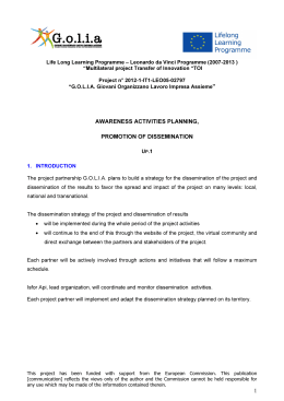
Chapter 1. Introduction
Figure 1.0.1: MODAClouds vision
project, which proposes a Model-Driven Approach for the design and execution of applications on multiple clouds [81]. MODAClouds aims at solving
the most relevant issues related to the cloud and, in order to achieve this
goal, it uses meta-models to represent and generalize cloud systems at different levels of abstraction. According to the MODAClouds vision (Figure
1.0.1), we can distinguish three types of meta-models: the Computation Independent Model (CIM), the Cloud Provider Independent Model (CPIM)
and the Cloud Provider Specific Model (CPSM).
The approach we have used is different from the ones which are generally
adopted by other several cloud related projects. In the next chapter we will
discuss about such projects and approaches, which are generally based on
multi-cloud libraries, so they try to face cloud issues like interoperability,
compatibility and portability working at API level.
In Section 1.1 we introduce the context providing a definition of Cloud
Computing and describing its general features. Then we will discuss about
the objectives of this thesis in Section 1.2 and we will anticipate the achieved
2
1.1 The Cloud Computing
Chapter 1. Introduction
results in Section 1.3. Finally, Section 1.4 outlines the structure of this thesis.
1.1
The Cloud Computing
Nowadays there are several definitions of Cloud Computing, but the one given
by the National Institute of Standard Technology (NIST) looks the most
accurate [1]:
Cloud computing is a model for enabling ubiquitous, convenient, on-demand network access to a shared pool of configurable
computing resources (e.g., networks, servers, storage, applications, and services) that can be rapidly provisioned and released
with minimal management effort or service provider interaction.
This definition highlights the basic properties of Cloud Computing:
• Ubiquity: the user can totally ignore the location of the hardware infrastructure hosting the required service and can use the service everywhere and every time through his client application.
• Convenience: the consumer can use a service exploiting remote physical
resources, without necessity of buying/acquiring those resources. He
just uses the resources provided by the provider and pays for them with
a pay-per-use mechanism.
• On-demand activation: a service consumes resources only when is explicitly activated by the user, otherwise it is considered inactive and
the resources needed for its execution can be used for other purposes.
The NIST definition also specifies five essential characteristics of Cloud Computing:
• On-demand self-service: a consumer can use the resources without any
interaction with the service provider, with an on-demand policy.
3
1.1 The Cloud Computing
Chapter 1. Introduction
• Broad network access: resources are available through the Internet and
can be accessed through mechanisms that promote their use by simple
(thin) or complex (thick) clients.
• Resource pooling: physical and virtual resources are pooled to serve
many users and are dynamically assigned with respect to the users’
needs and requirements.
• Rapid elasticity: resources can be rapidly and elastically provisioned;
the consumer often perceives “unlimited” resources that can be purchased in a very short time.
• Measured service: resources use is always automatically controlled and
optimized by monitoring mechanisms at a level of abstraction appropriate to the type of service (e.g., CPU activity time for processing
services and so on).
We can distinguish three main service models in the world of Cloud Computing:
• Software-as-a-Service (SaaS): the consumer uses a provider’s application running on a cloud infrastructure. The user can manage only
limited user-specific application settings and cannot control the underlying infrastructure.
• Platform-as-a-Service (Paas): the consumer can deploy on the cloud infrastructure owned or acquired applications created using programming
languages and tools supported by the provider. The user can control
the application and the deployment settings, but cannot manage the
underlying infrastructure, or the allocated resources.
• Infrastructure-as-a-Service (IaaS): the consumer can deploy and execute any kind of software on the cloud infrastructure. The user cannot
control the underlying infrastructure, but has control over the deployed
applications, Operating System, storage, and some network components (e.g., firewalls) and it is responsible of the management of the
resources.
4
1.2 Objectives
Chapter 1. Introduction
Finally, we can distinguish different deployment models:
• Public Cloud: the cloud infrastructure is made available to the general
public and is owned by a private organization selling cloud services.
• Community Cloud: the cloud infrastructure is shared among several
organizations and supports a specific community with shared concerns.
It can be managed by the organizations or a third party and may exists
on-premise or off-premise.
• Private Cloud: the cloud infrastructure can be accessed only within the
organization and can be managed by the organization itself or a third
party and may exists on-premise or off-premise.
• Hybrid Cloud: the cloud infrastructure is composed by different autonomous clouds connected together with a standard or proprietary
technology that enables data and application portability.
1.2
Objectives
The objective of this thesis is to exploit the model-driven approach proposed by
MODAClouds in order to define suitable meta-models at different abstraction
levels, oriented to cloud systems modelling and their performance and costs
evaluation.
As we has seen, the Cloud Computing can offer many interesting features,
but at the same time it may introduce some non-negligible issues. Two
relevant issues are about performance and cost of systems and applications
deployed on the cloud. Nowadays there are a lot of cloud providers and each
of them offers a proprietary cloud infrastructures with certain configurations
and cost profiles. Cloud users should be able to compare different providers
against costs and performance, in order to select the best solution(s). So, in
the most general case, cloud users should take into account several different
architectures and should be able to evaluate costs and performance for each
of them. This task can be very complex and unfeasable if it is carried on
5
1.3 Achieved Results
Chapter 1. Introduction
manually, because the number of possible solutions, given by the available
providers and the metrics of interests, can become very high.
To face this problem, automatic or semi-automatic cost and performance
evaluation tools are needed. Nowadays there exist different tools which allow to carry on cost and performance analysis on proprietary systems, but
they do not support cloud systems. For example, in this thesis we will refer
to the Palladio Framework, which supports performance analysis for proprietary systems, but does not natively support neither cost estimation, neither
cloud systems. The reason of this lack of support of cloud systems is due to
the difficulty to find a common representation of cloud services in terms of
provided cost and performance. In the next chapter we will discuss about the
existing tools which allow to run performance and cost analyses in different
contexts, but we will make use of the Palladio Framework, as we will see
later.
1.3
Achieved Results
Several results have been achieved while trying to reach the goal of this thesis:
• We have analyzed cloud services, cost profiles and scaling policies of
Google, Microsoft, Amazon and Flexiscale. The obtained results have
been useful to derive the general cloud meta-model (CPIM) and to
derive a suitable cost representation.
• We have defined the CPIM and the CPSMs related to Amazon, Google
and Microsoft. The CPSMs have been derived using the general concepts represented in the CPIM. Also, a guideline to derive CPSMs
starting from the CPIM is provided, taking as example the derivation
of the CPSM related to Flexiscale.
• In order to use Palladio for performance and cost analyses, we have provided a mapping between the concepts defined within the CPIM/CPSMs
and the ones defined within the Palladio Resource Model.
6
1.4 Structure of the thesis
Chapter 1. Introduction
• Finally, a Java tool has been implemented in order to extend Palladio,
allowing to run semi-automatic 24-hours analyses and to include cost
estimations within them. We have also tested the Java tool in order to
make a comparison between Amazon and Flexiscale.
1.4
Structure of the thesis
This thesis is structured as follows.
The state of the art is described in Chapter 2, in which the main approaches to ensure interoperability and compatibility among heterogeneous
cloud systems are presented. In this chapter we will also describe several
cloud-related projects and multi-cloud libraries which follow these approaches
and we will present some existing tools used for performance and cost evaluation.
Chapter 3 is about the Palladio Framework we have extended and used
for performance and cost analyses.
In Chapter 4 we report the analysis about cloud services, cost profiles
and scaling policies of the cloud systems owned by Amazon, Google and
Microsoft.
The general cloud meta-model (CPIM) and its specific derivations (CPSMs)
for amazon, Google and Microsoft are presented in Chapter 5.
In Chapter 6 we present the mapping which allow to represent cloud resources within Palladio. Also an example for the Amazon, Google, Microsoft
cloud providers is presented.
Chapter 7 describes the Java tool we have implemented to extend Palladio
in order to consider 24-hours analyses and cost estimations. The tool has
been tested using a Palladio representation of the SpecWeb 2005 benchmark
and the results are presented in Chapter 8.
7
Chapter 2
State of the Art
In this chapter we will give a general overview of the cloud, discussing about
different types of interoperability between cloud infrastructures. We will also
provide some information about multi-cloud libraries which allow to improve
the interoperability between different clouds operating at a low abstraction
level. Also some cloud-related projects are presented. They try to face some
relevant issues related to cloud computing at different level of abstractions.
Some of these problems are outlined in Section 2.1, which describes also the
kinds of interoperability between different clouds.
In Section 2.2 we will provide more detailed information about the cloud
libraries jclouds, d-cloud, fog and Apache libcloud.
Section 2.3 provides an overview of the 4CaaSt project, that follows the
Multi-Cloud approach. We will provide a brief description of the framework,
of the architecture and of the general functioning.
Section 2.4 describes the Open Cloud Computing Interface (OCCI), a
library that provides several functionalities to face the problem of interoperability with the Inter-Cloud approach.
Section 2.5 and Section 2.6 describe the mOSAIC and Optimis projects,
their general architecture and their functioning. They both provide features
to manage cloud services and applications with the Sky-Computing approach.
Section 2.7 is about the Cloud4SOA project which aims to guarantee
cloud interoperability and portability through a semantic approach.
8
2.1 Overview of the Cloud
Chapter 2. State of the Art
In Section 2.8 we will discuss about the existing model-driven feedback
provisioning tools for software systems.
Finally, in Section 2.9 we will make some final considerations about the
differences between our approach and the ones discussed in this chapter.
2.1
Overview of the Cloud
At the present time, the main problem in the world of cloud computing is
the absence of common standards. This leads on the one hand to a lack of
uniformity and on the other to a large amount of proprietary incompatible
solutions.
We can identify several common weaknesses among the actually available
cloud services:
• Often there’s no way to manage the Service Level Agreements (SLAs)
and to monitor the Quality of Service (QoS).
• Lack of infrastructural uniformity and interoperability among different
cloud providers.
• Lack of software uniformity (different platforms and APIs) among different cloud providers.
• Security issues on access and use of cloud services.
Research in field of cloud computing is focusing mostly on the resolution of
these issues. This thesis is focused on the first three issues. In this context,
we can classify other literature proposals according to the following research
lines:
• QoS-aware clouds
• Inter-Cloud (cloud federation, cloud bursting, cloud brokerage)
• Multi-Cloud (cloud brokerage)
• Sky-Computing
9
2.1 Overview of the Cloud
Chapter 2. State of the Art
The first one is referred to the projects aimed to add new features of SLA
acknowledgment and QoS monitoring to the cloud infrastructures. These
features are essential for several kinds of applications (e.g., real-time, timecritical and so on), so that we cannot use all the cloud capabilities if we are
not able to manage them. For this reason there are many running projects
aimed to realize frameworks for SLA management and QoS monitoring.
The term Inter-Cloud has a similar meaning with respect to the term
Internet: Internet is a “net of nets”, that is a set of heterogeneous nets
characterized by interoperability [2, 3]. In the same way, Inter-Cloud is a
“cloud of clouds”, that is a set of different clouds that are able to communicate
and to share resources. A cloud federation is a set of clouds bound together
and able to communicate and to share resources, so this term is often used
as a synonym of Inter-Cloud. The target of resource sharing cannot be
achieved without a strong integration at IaaS level between different cloud
providers. This kind of integration can be applied within a homogeneous
cloud environment, in which all the clouds belong to the same deployment
model, or even in a heterogeneous one, in which can coexist private and
public clouds. Referring to the last scenario, the hybrid cloud deployment
model can be considered a particular form of Inter-Cloud. Within a cloud
federation a cloud provider can “burst” into another one when the demand
for computing capacity spikes. This practice is called cloud bursting and
can be considered a technology similar to the load balancing, but applied
among different clouds. In general, within a cloud federation is possible to
share every kind of resources, even if the most common and appreciated
feature is that regarding VMs mobility. With the expression VMs mobility is
intended that we can move applications from a VM to another belonging to
a different cloud within the same cloud federation. There are many reasons
to do this, for example to achieve more resilience or better performance for
our applications.
The term Multi-Cloud is quite new in the world of cloud computing and
it can be referred to the way of deploying and evolving an application using
different cloud providers [4]. In a Multi-Cloud infrastructure an application can be deployed on different clouds which likely have different APIs
10
2.1 Overview of the Cloud
Chapter 2. State of the Art
and deployment models (e.g., public, private, and so on). Furthermore, in
this context an application can incorporate new clouds as they appear and
can manage the resources applying several mechanisms (e.g., load balancing,
VM migration and so on). All these features can be provided only through
the integration and the standardization of the cloud-specific interfaces. A
Multi-Cloud infrastructure can improve the following cloud-based application characteristics:
• Reliability: by deploying an application on multiple clouds, we create
redundancy, so that we can improve the application resilience.
• Portability: when we develop a new cloud-based application we may
incur into the so-called lock-in. Since many cloud providers have their
own proprietary platforms and APIs, if we want deploy or migrate our
application into a different cloud, we cannot do it if the platform and
API of the new cloud are incompatible with the previous one. The
result is that our application is “locked in” the first cloud we have
chosen. This phenomenon cannot occur in a cloud environment with a
standard, unified interface such as a Multi-Cloud infrastructure.
• Performance: let’s consider an environment where an application is
deployed on different cloud providers. In this context we can apply load
balancing both locally (within a cloud provider) and globally (among
the different cloud infrastructures). In the last case, we can simply
consider to migrate an instance of our application from a cloud to
another one with better performance.
In the context of Multi-Cloud and Inter-Cloud, the term cloud brokerage
refers to the way of choosing a certain cloud provider with negotiation. A
special entity called broker acts as a negotiator to select a suitable cloud
provider according to the application requirements. So the broker hides the
implementation details of the Multi-Cloud or Inter-Cloud infrastructure from
the user. Moreover, the user perceives a single entry-point to the cloud
resources.
11
2.1 Overview of the Cloud
Chapter 2. State of the Art
The last research area is that regarding the so-called Sky-Computing, a
particular architecture laying above the cloud computing architecture. It
is a sort of middleware that control and manage an environment of clouds,
offering variable storage and computing capabilities [5, 6]. In other words,
it consists in the interconnection and provisioning of cloud services from
multiple domains. So it combines the infrastructural interoperability, typical
of an Inter-Cloud architecture, and the uniformity at PaaS level, typical of
a Multi-Cloud infrastructure. The Sky-Computing aims to maximize the
interoperability among the clouds and to achieve the maximum elasticity for
the cloud-based applications and services. Finally, within a Sky-Computing
architecture it is possible to perform SLA management and QoS monitoring,
so such an architecture is particularly suitable to realize High Performance
Computing (HPC) systems.
The Figure 2.1.1 shows the state of the art in the previously described
areas and highlights the classification of the open-source projects that will
be analyzed in the following.
There are several specific projects for the SLA management and QoS
monitoring, but in general these problems are faced in most of the projects
in the fields of Inter-Cloud and Multi-Cloud. However, the specific ones are
the followings:
• SLA@SOI [7, 8]: an European project belonging to the Seventh Framework Programme (FP7), aimed at the realization of a framework for
SLA management in the Service Oriented Infrastructures (SOIs). The
framework supports a multi-layered SLA management, where SLAs
can be composed and decomposed along functional and organizational
domains. Other important features are the complete support of SLA
and service lifecycles and the possibility to manage flexible deployment
setups.
• IRMOS [9, 10]: an European FP7 project for SLA management in realtime interactive multimedia applications on SOI systems. The framework is composed by offline and online modules which can respectively
perform offline and online operations. It supports the offline perfor12
2.1 Overview of the Cloud
Chapter 2. State of the Art
Figure 2.1.1: State of the art
mance estimation and online features such as the SLA and workflow
dynamic management, the performance evaluation and monitoring, the
redundancy and support to migration in order to increase the application resilience.
In the field of Multi-Cloud we have considered the following projects and
libraries:
• jclouds [11] (Subsection 2.2.1): is an open-source Java library that
allows to use portable abstraction or cloud-specific features at the IaaS
layer.
• d-cloud [13] (Subsection 2.2.2): is an open-source API that abstract
the differences between clouds at IaaS level.
• fog [15] (Subsection 2.2.3): is an open-source Ruby library that facilitates cross service compatibility at IaaS level.
13
2.1 Overview of the Cloud
Chapter 2. State of the Art
• Apache Libcloud [16] (Subsection 2.2.4): is an open-source standard
Python library that abstracts away differences among multiple cloud
provider APIs at IaaS level.
• 4CaaSt [17]: is an European FP7 project described in Section 2.3. It
provides a framework that supports the creation of advanced cloud
PaaS architectures. It operates both at IaaS and Paas levels.
The followings are the projects related to the field of Inter-Cloud (IaaS level):
• Reservoir (Resources and Services Virtualization without Barriers) [20]:
is a framework that enables resource sharing among different clouds,
is an European FP7 project. The framework supports a distributed
management of the virtual infrastructures across sites supporting private, public and hybrid cloud architectures. It is also defined a formal
Service Definition Language to support service deployment and life cycle management across Reservoir sites. Other important features are
the Automated Service Lifecycle management for service provisioning
and dynamic scalability, and the possibility to use algorithms for the
allocation of resources to conform to SLA requirements.
• OpenNebula [21]: is an open-source project aimed at building the industry standard open source cloud computing tool to manage the complexity and heterogeneity of distributed data center infrastructures. It
gives the possibility to use multi-tenancy and to control and monitor physical and virtual infrastructures. It also enables hybrid cloud
computing architectures and cloud-bursting. Finally, the framework
is characterized by reliability, efficiency and massive scalability, and
makes use of multiple open and proprietary interfaces (OCCI, EC2
and so on).
• OCCI (Open Cloud Computing Interface) [22]: a set of specification
for REST-based protocols and APIs aimed at interoperability among
different clouds, described in Section 2.4.
14
2.2 Multi-Cloud Libraries
Chapter 2. State of the Art
The presence of several projects in the field of Sky-Computing highlights the
importance of standardization and integration in the world of cloud computing. In this context, we have considered the following projects:
• mOSAIC [29]: an FP7 project described in Section2.5. It is an opensource API and platform for multiple clouds, operating at PaaS and
IaaS levels.
• CONTRAIL [32]: an FP7 project on cloud federation. It is aimed
at avoiding lock-in, thanks to support to application migration. It
provides a complete environment that support the creation of federated
IaaS and PaaS systems.
• NIMBUS [28]: project aimed at realization of IaaS infrastructures. It
supports multiple protocols (WSRF, EC2 and so on) and it gives the
ability to define environments that support Multi-Cloud. The framework provides the possibility to define clusters in an easy way and
supports remote deployment and VMs lifecycle management. It is also
possible to have a fine-grained control of resource allocation on VMs.
• Optimis [33]: an FP7 project described in Section 2.6. It provides a
framework for flexible provisioning of cloud services. It operates both
at PaaS and IaaS levels.
• Cloud4SOA [35]: an FP7 project aimed at enhancing cloud-based application development, deployment and migration. It tries to achieve
interoperability by semantically interconnecting heterogeneous services
at PaaS level (see Section 2.7).
2.2
Multi-Cloud Libraries
In this section some open-source libraries used for Multi-Cloud projects and
applications will be discussed. They all provide an API that abstracts the
differences between different clouds. Notice that all these libraries are aimed
at resolving differences between clouds at IaaS level, not at PaaS level, so
15
2.2 Multi-Cloud Libraries
Chapter 2. State of the Art
they don’t offer all the services needed in a Multi-Cloud framework, such
as monitoring of QoS, cloud brokerage and so on. Thus, the portability
of the applications is guaranteed under the hypothesis that they have been
developed using standard platforms and APIs integrated with the libraries
described in the following subsections.
As a counterexample, if we develop an application on Google AppEngine
using the Google’s proprietary APIs, there’s no way to perform the migration
or the deployment of the application to a different cloud using only the features offered by the following libraries. This task can be performed by more
advanced frameworks which works even at PaaS level and often integrate
these libraries to manage the IaaS level.
2.2.1
The Jclouds Library
The jclouds library gives an abstraction of about 30 different cloud providers
and can be used for developing application using the Java or Clojure 1 programming languages. The library offers several functionalities for the following services [11]:
• Blobstore (Blobstore API): provides the communication with the storage services based on the key-value mechanism (e.g., Amazon S3, Google
BlobStore and so on).
• Computeservice (Compute API): simplifies the management of virtual
machines (VMs) on the cloud.
The Table 2.1 shows which cloud providers are supported with respect to the
APIs provided by jclouds.
The Compute API aims to simplify the management of VMs and support and integrate the Maven and Ant tools. The API is location-aware, so
it is not needed to establish multiple connections in the multi-homed cloud
architectures. It is also possible to define node clusters that can be managed
as a single entity, and to run scripts on these clusters handling the execution
errors through special exceptions types. If the user wants to test a service
1
http: // clojure. org/
16
2.2 Multi-Cloud Libraries
Chapter 2. State of the Art
Compute API
Blobstore API
aws-ec2
aws-s3
gogrid
cloudfiles-us
cloudservers-us
cloudfiles-ok
stub (in-memory)
filesystem
deltacloud
azureblob
cloudservers-uk
atmos (generic)
vcloud (generic)
synaptic-storage
ec2 (generic)
scaleup-storage
byon
cloudonestorage
nova
walrus (generic)
trmk-ecloud
googlestorage
trmk-vcloudexpress
ninefold-storage
eucalyptus (generic)
scality-rs2 (generic)
cloudsigma-zrh
hosteurope-storage
elasticstack (generic)
tiscali-storage
bluelock-vclouddirector
eucalyptus-partnercloud-s3
slicehost
swift (generic)
eucalyptus-partnercloud-ec2
transient (in-memory)
elastichosts-lon-p (Peer 1)
elastichosts-sat-p (Peer 1)
elastichosts-lon-b (BlueSquare)
openhosting-east1
serverlove-z1-man
skalicloud-sdg-my
Table 2.1: jclouds - List of supported cloud providers
17
2.2 Multi-Cloud Libraries
Chapter 2. State of the Art
before the real implementation, he can use the stub classes provided by the
stub service. These classes can be bound to the in-memory blobstore to do
testing on services before their deployment. Finally, it is also possible to
persist node credentials in the blobstore to keep track of all of them.
The definition of the so-called Templates represents a form of support to
Multi-Cloud, because they encapsulate the requirements of the nodes so that
similar configurations can be launched in other clouds. A Template consists
of the following elements:
• Image: that defines which bytes boot the node(s), and details like the
operating system.
• Hardware: defines CPU, memory, disk and supported architecture.
• Location: defines the region or datacenter in which the node(s) should
run.
• Options: defines optional parameters such as scripts to execute at boot
time, inbound ports to open and so on.
The Blobstore API provides access to the management of key-value storage
services, such as Microsoft Azure Blob Service and Amazon S3. The API is
location-aware like the Compute API previously described. It is possible to
use the storage service in synchronous or asynchronous mode and the service
can be accessed by Java clients or even by non-Java clients through HTTP
requests. The API also supplies a Transient Provider, that is a local blobstore
that can be used to test services and applications before the deployment on
the cloud. There’s no difference, from the point of view of the API, between
local and remote storage, as they are accessed in the same way.
A Blobstore consists of different containers, each of which can contain
different storage units called blobs. Blobs cannot exist for themselves but
they always belong to a container.
The library jclouds also provides another way of enabling the multi-cloud:
it is possible to use the open-source tool Apache Karaf. This tool is a small
OSGi based runtime which provides a lightweight container onto which various components and applications can be deployed [12]. It can manage the hot
18
2.2 Multi-Cloud Libraries
Chapter 2. State of the Art
deployment of the application and the dynamic configuration of services, it
offers a logging system supported by Log4J and a security framework based
on JAAS. Finally, the main feature is the possibility to manage multiple
instances through the Karaf console.
The Karaf environment can be extended with the so-called features. The
library jclouds integrates several cloud libraries which can be installed in
Karaf as features, so that it is possible to use this tool to manage the instances. The set of supported clouds for the tool Karaf is a subset of that
reported in the Table 2.1.
Appendix A contains more detailed information and practical examples
of use of both the Compute and the Blobstore APIs.
2.2.2
The d-cloud Library
According to the official definition, d-cloud is an API that abstract the differences between clouds [13]. Even in this case, resources are divided into
two main categories:
• Compute: represents all the services associated to the computational
resources. The Figure 2.2.1 shows which compute services can be used
from each of all the supported cloud providers.
• Storage: represents all the services associated to the storage resources.
The Figure 2.2.2 shows which storage services can be used from each
of all the supported cloud providers.
The API is implemented in the Ruby programming language, but it expose an interface based on the REST (REpresentational State Transfer) software architecture, so we can define it a RESTful API (Figure 2.2.3). The
REST technology is platform and language independent, is based on standard protocols such as HTTP and is characterized by lower overhead and
complexity with respect to other similar technologies and protocols (e.g.,
SOAP, RPC and so on) [14].
19
2.2 Multi-Cloud Libraries
Chapter 2. State of the Art
Figure 2.2.1: d-cloud - Available Compute Services
Figure 2.2.2: d-cloud - Available Storage Services
Figure 2.2.3: d-cloud - Overview
20
2.2 Multi-Cloud Libraries
Chapter 2. State of the Art
The d-cloud REST interface can be used through the d-cloud client or
whatever HTTP client, such as cURL2 . With the chosen client is possible
to send requests to the specific d-cloud server launched for a certain cloud
provider.
See Appendix A for more detailed information about the structure of the
Compute and Storage services or to have a view on how to implement their
functionalities.
2.2.3
The Fog Library
The Ruby library Fog offers several features similar to the ones offered by the
libraries previously described. The functional classification of the available
features is described in the following:
• CDN (Content Delivery Network): it includes all the services that
makes possible to create content distribution networks, in order to improve the performance by moving data closer to the final user.
• Compute: it represents the basic service to have access to the computational resources.
• DNS (Domain Name System): it is the service responsible for service
addressing.
• Storage: it is the basic storage service.
The Table 2.2 shows which fog services are available on the supported cloud
providers.
Examples of implementations of these services are available in Appendix
A.
2.2.4
The Apache Libcloud Library
The library libcloud by Apache is defined as a unified interface to the cloud
and as a standard Python library that abstracts away differences among
2
http://curl.haxx.se/
21
2.2 Multi-Cloud Libraries
Provider
Amazon Web Services (AWS)
BlueBox
BrightBox
Clodo
DNSimple
DNS Made Easy
Dynect
Ecloud
Glesys
GoGrid
Google
Libvirt
Linode
Local
NewServers
Ninefold
OpenStack
RackSpace
Slicehost
Storm On Demand
VCloud
VirtualBox
Vmfusion
Voxel
Vsphere
Zerigo
Chapter 2. State of the Art
CDN
Compute
DNS
Storage
!
%
%
%
%
%
%
%
%
%
%
%
%
%
%
%
%
!
%
%
%
%
%
%
%
%
!
!
!
!
%
%
%
!
!
!
%
!
!
%
!
!
!
!
!
!
!
!
!
!
!
%
!
!
%
%
!
!
!
%
%
%
%
%
!
%
%
%
%
!
!
%
%
%
%
%
%
!
!
%
%
%
%
%
%
%
%
%
!
%
%
!
%
!
%
!
%
%
%
%
%
%
%
%
Table 2.2: fog - Cloud Providers and Supported Services
22
2.2 Multi-Cloud Libraries
Chapter 2. State of the Art
multiple cloud provider APIs [16]. The current version3 provides the following
features:
• Cloud Servers (in the branch libcloud.compute.*): it is a Compute
Service, so it supports the computational services furnished by cloud
providers, such as Amazon EC2 and Rackspace CloudServers. The
Table 2.3 shows which services are available for the supported cloud
providers.
• Cloud Storage (in the branch libcloud.storage.*): supports the storage
service provided by Amazon S3 and Rackspace CloudFiles. It includes
several services for the management of containers (list, create and delete
containers) and objects (list, upload, download and delete objects).
• Load Balancer as a Service (LBaaS, in the branch libcloud.loadbalancer.*):
actually, this feature is supported only by Rackspace US and GoGrid. It
includes the services needed to create load balancers and to attach/detach them to/from members and compute nodes.
For more details about the implementation of these services, see Appendix
A.
3
The last stable version is the 0.5.2, but there is also the version 0.6.0-beta1
23
2.2 Multi-Cloud Libraries
Provider
Bluebox
Brightbox
CloudSigma
Dreamhost
EC2
enomaly ECP
ElasticHosts
Eucalyptus
Gandi.net
GoGrid
IBM Cloud
Linode
Nimbus
OpenNebula
OpenStack
OpSource Cloud
Rackspace
RimuHosting
serverlove
skalicloud
Slicehost
SoftLayer
Terremark
vCloud
Voxel
VPS.net
Chapter 2. State of the Art
list
reboot
create
destroy
images
sizes
deploy
!
!
!
!
!
!
!
!
!
!
!
!
!
!
!
!
!
!
!
!
!
!
!
!
!
!
!
%
!
!
!
!
!
!
!
!
!
!
!
!
!
!
!
!
!
!
!
!
!
!
!
!
!
!
!
!
!
!
!
!
!
!
!
!
!
!
!
!
!
!
!
!
!
!
!
!
!
!
!
!
!
!
!
!
!
!
!
!
!
!
!
!
!
!
!
!
!
!
!
!
!
!
!
!
!
!
!
!
!
!
!
!
!
!
!
!
!
!
!
!
!
!
!
!
!
!
!
!
!
!
!
!
!
!
!
!
!
!
!
!
!
!
!
!
!
!
!
!
!
!
!
!
!
!
!
!
%
%
%
%
!
!
!
%
!
!
%
!
!
!
!
!
!
%
!
!
!
!
!
!
%
%
Table 2.3: libcloud - Supported Compute Services and Cloud Providers
24
2.3 The 4CaaSt Project
2.3
Chapter 2. State of the Art
The 4CaaSt Project
The European FP7 project 4CaaSt aims to realize a framework that supports the creation of advanced cloud PaaS architectures. In order to reach
this objective, the project provides a high level of abstraction of the hosting
by hiding its complexity. Programming libraries and interfaces are also provided in order to simplify the development of new applications, which can
be monitored at runtime and managed during their entire lifecycle.
In the official documentation [18] emerges the distinction between Service
Providers (SP) and Platform Providers (PP).
A service provider can receive several benefits using the 4CaaSt framework, such as the possibility to use a specific formalism called Blueprint to design services specifying their requirements. As we will see later, the blueprint
can be used to solve the lock-in issue. The framework also supports cloud
technologies for automatic scalability, multi-tenancy and resource optimization. It is also possible to extend the IaaS layer with Network-as-a-Service
(NaaS) functionalities, which can be used to define custom net topologies.
A service provider can use the so-called 4CaaSt Marketplace, that enables
the unified access to all kind of XaaS services. Within the marketplace it
is possible to buy services, applications and components which simplify the
process of the application make-up.
A platform provider can use the framework to develop PaaS solutions in
an easy way and can have a unified management view of all the different
technologies used. The features of the marketplace can be also exploited
by the platform providers to promote the development of dynamic business
ecosystems in which several service providers can develop and provide new
services in a relatively short time.
The overall 4CaaSt architecture is shown in Figure 2.3.1, in which can be
distinguished the following layers: Service, Resource, Provisioning.
The Service Layer provides a Web GUI and a PaaS API for the final
users and includes several features to manage and monitor the services. It is
composed by the following modules:
• eMarketPlace, that manages the offers about the services available for
25
2.3 The 4CaaSt Project
Chapter 2. State of the Art
Figure 2.3.1: 4CaaSt - Overall Architecture
the final user in the 4CaaSt platform.
• Service Lifecycle Manager (Figure 2.3.2), that manages the service lifecycle, that roughly consist in development, deployment, testing & monitoring. In these phases the service blueprint is, respectively, created,
consulted and updated. This module answers to the requests of service retrieval received by the eMarketplace: the service is selected by
the Resolution Engine depending on the compatibility between the
blueprint and the specified requirements; the execution environment
is monitored by the Feedback Engine in order to update the blueprint
if needed; the Provisioning Manager requests to the Resource Manager the resources needed to instantiate the service, on the basis of the
blueprint content.
The Resource Layer is responsible for the management and the monitoring of the services and contains the Resource Manager module, that hides
the complexity of how platforms are provisioned and how these are connected
to other services. The platforms are encapsulated into Virtual Platforms,
which are adapters to the heterogeneous instances of possible platforms. In
26
2.3 The 4CaaSt Project
Chapter 2. State of the Art
Figure 2.3.2: 4CaaSt - Service Lifecycle Manager
the same way, a product is encapsulated into a Virtual Product, that provides a unique interface for all possible products. The Resource Manager
is responsible for selecting a suitable Virtual Platform for a given service,
and can allocate and deallocate the resources on the basis of the information
given by the deployment descriptor (derived from the blueprint). In order to
manage the resources, the Resource Manager has to communicate with the
underlying Provisioning Layer.
The Provisioning Layer is responsible for the allocation and deallocation of the resources, depending on the requests received by the Resource
Manager. It contains the following main modules:
• Runtime Execution Containers (RECs, Figure 2.3.3), which represents
the Virtual Machines (VMs) in which can be installed several products. A REC is responsible for the execution of Application Components (ACs), Product/Platform Instances (which are derived from
Virtual Products) and Product/Platform Instance Components (PICs).
PICs are particular platform technologies, such as JBoss, Apache Web
27
2.3 The 4CaaSt Project
Chapter 2. State of the Art
Figure 2.3.3: 4CaaSt - Example of REC
Server and so on, which can be used by ACs. RECs are managed by
the REC-Register, that keeps track of RECs and their type, moreover it
manages the links between the RECs and the load balancing operations
(REC distribution on different physical machines). Notice that Load
Balancers control the distribution, migration and replication of the Application Components. The REC Manager is used to manage centrally
the existing REC instances and to give to the Resource Manager a high
level access to them.
• Enabler Interfaces, which are interfaces for any kind of XaaS service
and can be integrated into the RECs or into the 4CaaSt platform.
They make possible the use of IaaS services needed for scalability and
migration, moreover they enable the use of NaaS services for the management of custom net topologies, which can be internal or external
and QoS-aware.
Within the architecture there are two common layers: Administration and
Monitoring. The first one can start/stop Product Instances (PIs), deploy/remove Application Components on a PI and migrate them from a PIC in a
REC to another PIC in another REC. It can also perform PICs configuration
and reconfiguration. The Monitoring Layer generates monitoring indicators
by statistics and data mining techniques and can communicate with the Re28
2.3 The 4CaaSt Project
Chapter 2. State of the Art
source Manager (Resource Layer) and the Service Lifecycle Manager (Service
Layer) to allow dynamic reaction to QoS changes and/or SLAs violations.
The Figure 2.3.4 shows the detailed structure of the application lifecycle
within the 4CaaSt Platform. First of all, the application/service is developed
by Engineers/Developers, which specify its structure and its requirements in
the Application Blueprint. The Blueprint Provider (corresponding to an Engineer or a Developer) specifies a new Target Blueprint using the Blueprint
Template. The output of this phase is an “unresolved” target blueprint containing resource constraints and the Virtual Abstract Topology (VAT). The
second phase is the target blueprint resolution, in which the blueprint provider can get access to a set of source blueprints available in the blueprint repository in order to use them to satisfy the constraints of the target blueprint.
The output of this phase is a “resolved” target blueprint, with a resolved VAT
in which all the constraints are replaced with the retrieved source blueprints.
After the resolution the resolved target blueprint is stored into the blueprint
repository. and it can be customized with a customer contract, that is a customization of the resolved VAT. Finally the resolved and customized target
blueprint is stored again into the blueprint repository and it can be deployed
and consumed. The resolved target blueprint and the customized one can be
reused as source blueprints in the following blueprint specifications.
The service publication in the marketplace is performed by the Service
Provider, who also defines the business terms associated to the service. In
this phase the resolved target blueprint is exposed in the marketplace.
After the publication, there is the contracting phase, performed by the
Marketplace Customer, who can customize the application, the SLAs, the
price and so on. The set of these customizations represents the customer
contract that can be used to modify the resolved target blueprint. The
resolved VAT is customized according to the contract so the result of this
phase is a customized, resolved target blueprint.
Once the service has been customized, it can be delivered, that is it can be
deployed on the platform, together with the resolved and customized target
blueprint.
Finally, the service is executed and adaptation, accounting, billing can be
29
2.4 The OCCI Interface
Chapter 2. State of the Art
Figure 2.3.4: 4CaaSt - Application Lifecycle
performed involving the Marketplace Customer and the Service Customer.
The former manages the service and is responsible for adaptation, while
the latter represents the end-user accessing the service and is subjected to
accounting and billing.
For what concerning data management, the 4CaaSt platform supports
and extends the open-source key-value store Scalaris4 [19]. So it is possible
to add new nodes to an existing data store deployment (scale-out) or to
remove existing nodes with graceful data migration (scale-in).
The features offered by 4CaaSt are compatible only with 4CaaSt-compliant
providers, which belong to the 4CaaSt Consortium or simply implements the
4CaaSt platform.
2.4
The OCCI Interface
The term OCCI stands for Open Cloud Computing Interface and it is referred
to a set of specifications defined to realize RESTful API and protocols for the
management of cloud infrastructures [22]. The specifications are driven by
4
http://code.google.com/p/scalaris/
30
2.4 The OCCI Interface
Chapter 2. State of the Art
the Open Grid Forum 5 , an open community that aims to guarantee a rapid
evolution and adoption of applied distributed computing.
There are three types of specifications:
1. OCCI Core [23]: it defines the OCCI Core Model, that can interact
with different renderings (ways of interaction with the RESTful OCCI
API) and can be extended with new functionalities (extensions).
2. OCCI HTTP Rendering [24]: it defines the ways of interaction between
the OCCI Core Model and the RESTful OCCI API to make possible
the communication via HTTP.
3. OCCI Infrastructure [25]: it defines the extension OCCI Infrastructure
for the IaaS domain.
OCCI is defined as a boundary protocol and API that acts as a service frontend to a provider’s internal management framework [23]. The Figure 2.4.1
shows where is located OCCI in a context of interaction between a Service
Provider and a Service Consumer.
Notice that the term Service Consumer can be referred to both the final
user or a system instance.
The OCCI Core Model [23] defines a representation of instance types
which can be manipulated by a rendering implementation. In other words, it
includes an abstract representation of the available resources and of the information needed to the identification, classification, association and extension
of these resources. An essential characteristic of the OCCI Core Model is
that it can be extended in such a way that any extension will be visible at
runtime by an OCCI client. The extensions can be implemented with inheritance or using a “mix-in” like concept, that can be applied only at “object
level” (only to instances, never to types). A Mixin is a sort of abstract class
that provides a certain functionality to be inherited by a subclass and that
is not intended for instantiation.
In Figure 2.4.2 is shown the UML class diagram of the OCCI Core Model.
5
http://www.ogf.org/
31
2.4 The OCCI Interface
Chapter 2. State of the Art
Figure 2.4.1: OCCI - Overview
Figure 2.4.2: OCCI - Core Model
32
2.4 The OCCI Interface
Chapter 2. State of the Art
The heart of the model is the Resource type, that represents any resource
exposed by OCCI, such as virtual machines, jobs, users and so on. A Resource
can have several attributes, which are inherited by its subclasses, and can
be linked to other resources through the Link type. Both the Link and
Resource types are sub-types of the abstract type Entity. Each sub-type
of Entity is identified by a unique Kind instance and can be associated to
Mixin instances, which provide additional functionalities or capabilities. The
Mixin and Kind types are sub-types of the Category type and are composed
by Action instances, which represents invokable operations applicable to a
Resource type. The Category type is the basis of the type identification
mechanism: a Category instance belongs to a categorization scheme (the
attribute scheme) and has an identifier (the attribute term) that is unique
within the scheme. So it is possible to address any type of the Core Model by
concatenating its categorization scheme with its category term, e.g. http://
example.com/category/schema#term. An important concept of the OCCI
Core Model is the mutability: attributes of a type can be either client mutable
or client immutable. In the first case, a client can specify the value of the
attributes when it creates a new instance and can update them at runtime,
so the server must support these operations; in the second case, instead, only
the server can manage the attributes of an instance.
The OCCI HTTP Rendering [24] specifies the interactions between
the RESTful API and the Core Model, so that it is possible to address
resources and actions through HTTP requests.
Once an entry point is defined, the client can discover the information
about the particular OCCI model implemented, deriving from the extension
of the OCCI Core Model. Since the Core Model is dynamically extendible, the
client can perform a dynamic detecting of the available categories and entities
with a query command (“/-/”). This operation is called bootstrapping.
The OCCI Core Model is not so interesting nor useful without considering
the OCCI Infrastructure extension, that provides all the basic features to
manipulate cloud resources at IaaS level. The Core Model is extended with
five additional classes: Network, Compute and Storage which extend the
class Resource; StorageLink and NetworkInterface which extend the class
33
2.5 The mOSAIC Project
Chapter 2. State of the Art
Link. The names of these new classes also correspond to their respective
terms (with the first letter de-capitalized). The Network type represents a
networking entity operating at level 2 (datalink) of the standard ISO/OSI
stack, but can be extended with the mixin mechanism to support the capabilities of level 3/4, such as TCP/IP. The Compute type represents a generic
computational resource, such as a virtual machine, while the Storage type
represents resources which can persist data into storage devices. In order
to create virtual data centers or virtual clusters it is possible to use the
StorageLink and NetworkInterface types. The first one allows to connect a
Resource instance to a target Storage instance, while the second one represents a sort of network adapter that allows to connect a Resource instance
to a Network instance. The NetworkInterface type is intended to be used
at level 2, but can be extended to support level 3, as already seen for the
Network type.
Notice that the OCCI Infrastructure also supports the definition of the
Infrastructure Templates, which represents predefined configurations of the
OCCI Infrastructure types. Actually, there are two types of supported templates: OS Template and Resource Template. The first one defines which
Operating System must be installed on a Compute resource, while the second one defines a preset Resource configuration.
The OCCI specifications are currently implemented by the following projects: jclouds (Subsection 2.2.1), Reservoir, OpenNebula.org, SLA@SOI, and
others.
2.5
The mOSAIC Project
The European project mOSAIC belongs to the Seventh Framework Programme (FP7) and it is an open-source API and platform for multiple clouds,
according to the official definition [29, 30]. The R&D of mOSAIC is focused
on the following weaknesses which characterize the actual cloud computing
infrastructures:
• Lack of common programming models for cloud-oriented applications.
34
2.5 The mOSAIC Project
Chapter 2. State of the Art
• Lack of tools for easy deployment of scalable applications and multicloud-based service compositions.
• Lack of standard interfaces for resource virtualization.
• Lack of SLA management and negotiation.
• Platform dependability and non-portability due to different APIs (lockin issue).
Notice that the first two points represent general issues related to the applications development and deployment, while the others represent the main
issues faced by, respectively, Inter-Cloud, QoS-aware and Multi-Cloud architectures.
The mOSAIC platform has been designed to benefit different types of
users. A final user can have a transparent and easy access to the resources
in order to avoid the lock-in issue, while a developer can use a consistent,
uniform and lightweight API that is platform- and language-independent.
An Administrator can easily manage the application lifecycle (deployment,
migration and update), while a new cloud provider can offer similar services
as the existing ones and can apply different business models for both IaaS
and PaaS levels.
The mOSAIC framework supports all the phases of a cloud-based application lifecycle, that is development, deployment, execution. The development support consists of the following modules and tools:
• Application Programming Interface (API), that provides the basic functionalities for the management of the storage services (file/block storage, column database), communication services (RPC, broadcast, multicast, streams and so on), monitoring services (application and resources state).
• Application tools, which consist of: deployment specification assistant,
workflow editor, Eclipse plug-in, and code examples. The first tool simplify the specification of the Application Deployment Descriptor providing template specifications which can be tuned by the user.
35
2.5 The mOSAIC Project
Chapter 2. State of the Art
Figure 2.5.1: mOSAIC - Cloud Ontology
• Cloud Ontology (Figure 2.5.1), that is a formal, symbolic representation of the cloud resources, on which is possible to apply a reasoning process. It includes different, specific ontologies, each of which is
referred to a particular domain. The Main Ontology represents the
general concepts and relationships related to cloud systems; the Domain Ontology gives a formal representation of the domain of services
and APIs; the APIs/Services Ontology describes the model, the profile
and the grounding for Cloud API; finally, the Requirements Ontology
represents the SLAs between cloud consumers and providers.
• Cloud usage patterns, which are used in the development phase in
combination with examples of use cases.
• Semantic Engine, that is responsible for the semantic mappings between the native ontology of a given cloud provider and the brokering
ontology defined in the framework. Furthermore, this module can perform ontological validation and translation.
The deployment support consists of the following modules:
36
2.5 The mOSAIC Project
Chapter 2. State of the Art
• Application Deployment Descriptor, that contains specific information
about the quantity, the operational availability, the QoS, the budget and the trade-off costs/performances associated to three types of
resources: computational (VMs and other computational services),
storage (file system, databases, virtual disks and so on), communication (message queue systems, communication between computational
nodes). The descriptor can be defined either manually by the user or
in a semi-automatic way using the mOSAIC Application Tools suite.
• Cloud Agency & Provider Agents (Figure 2.5.2), a multi-agent system responsible for SLA management (negotiation, renegotiation and
monitoring) that uses the Cloud Ontology to select the provider agents
suitable for the application deployment.
The execution support consists of the following components:
• Virtual Cluster (VC), it is created on the basis of the arranged SLA
and represents the set of computational resources associated to a given
application. This set can be modified both when a VC is created or at
runtime. A VC can be enriched by the Cloud Agency with monitoring
services useful to determine the QoS perceived by the user. So the
Cloud Agency can scale or move the application on the basis of QoS
changes, which can be caused not only by resource insufficiency, but
also by the definition of new SLAs by the user.
• Providers wrappers, a set of interfaces which allow the user to access
the cloud resources.
• Execution engine, that offers access methods to the reserved storage,
communication and computational resources inside a VC. This module
also offers a service to allocate the resources and another one to monitor
them.
The Application Programming Interface (Figure 2.5.3) has a layered
structure, in which the abstraction level follows an ascendent, bottom-up
ordering. The Native API & Protocol represents the lowest layer and contains
37
2.5 The mOSAIC Project
Chapter 2. State of the Art
Figure 2.5.2: mOSAIC - Cloud Agency
38
2.5 The mOSAIC Project
Chapter 2. State of the Art
Figure 2.5.3: mOSAIC - API Structure
the cloud-specific programming modules, which are different from cloud to
cloud. Above this layer there is the mOSAIC Middleware, that is a macrolayer that encapsulates the native provider’s API in order to create uniformity
at interface level. This macro-layer is composed by the Driver API and the
Interoperability API. The first one is a sort of wrapper of the basic features
offered by the native API, while the second one ensures the interoperability
between different programming languages. Finally there are the high level
APIs, which are directly exposed to the developer. This final macro-layer is
composed by the Connector API and the Cloudlet API. The Connector API
provides an abstract model of the cloud resources, depending on the chosen
programming language. The Cloudlet API, instead, provides a programming
model suitable for the use of the cloud resources (it is comparable with the
Java Servlet used in the J2EE framework).
Within the mOSAIC framework the applications are developed by composing the provided modules and can exploit the API to use the cloud resources. More precisely, an application is composed by:
• User components, which are defined by the developer.
39
2.5 The mOSAIC Project
Chapter 2. State of the Art
• Core components, the basic components provided by the platform.
• Miscellaneous components, which provide additional features.
• SLA components, which define the Service Level Agreements.
The typical lifecycle of a generic application within the mOSAIC Framework
is reported here in the following:
1. Application development.
2. Application deployment:
(a) Specification of the resource requirements in the Application Deployment Descriptor.
(b) Submission of the requirements to the Cloud Agency, that gives
back a resource contract committing to the requirements.
(c) Bootstrapping of the contracted resources.
(d) Application start.
3. Application execution:
(a) Monitoring.
(b) Scaling or moving according to the needs.
(c) Results gathering or real time interaction.
It is important to remark that the mOSAIC Framework acts as a sort of middleware for the cloud-based applications, but it also provides several features
which help the developers in the development phase. This is very important
to obtain well-structured, modular cloud applications, in which it is possible
to classify the components in two high-level categories: Cloud Components
and Cloud Resources. The firsts are building blocks defined and controlled
by the user, while the seconds are expected to be controlled by the cloud
providers. Having a modular application is necessary to guarantee efficiency
and micro-scalability, that is the possibility to optimize the resource usage
40
2.6 The Optimis Project
Chapter 2. State of the Art
by executing different components on the same virtual machine, in order to
exploit maximum computational capacity.
The considerations made until now hold even for what concerning the data
management. The Cloud Agency can act as a mediator for both the Compute
and Storage services, so it can scale or migrate data and applications in
the same way. Furthermore, mOSAIC gives special attention to the dataintensive applications in order to avoid the data lock-in issue. This is done
by using semantic ontologies and data processing to identify the application
requirements in terms of cloud data services [30].
The Figure 2.5.3 clearly shows that the mOSAIC API lays on the Native APIs of the supported cloud providers, so it works without any provider
side software support. The user never uses directly the Native APIs, but
always interact with the mOSAIC API. However, all the features offered by
the Cloud Agency work under the hypothesis of the availability of the provider’s ontology. This is not a trivial assumption, since nowadays there is no
uniformity in the way of representing cloud resources, even if there are some
projects which are trying to define a standard formal cloud ontology, such as
the Unified Cloud Interface (UCI) by the Cloud Computing Interoperability
Forum (CCIF).
2.6
The Optimis Project
The European project Optimis (Optimized Infrastructure Services) belongs
to the FP7 and aims to provide an open, scalable and reliable platform for
flexible provisioning of services [33, 34]. The platform can extend the existing functionalities through an automatic and adaptive service management,
based not only on the performance, but also on the so-called TREC factors:
Trust, Risk, Eco-efficiency, Cost. The final outcome of the project will be
a set of tools (Optimis Toolkit), which can be composed to realize different
types of cloud architectures.
The vision of Optimis can be found in the official documentation [34] and
it is based on the concept of cloud ecosystem (see the Figure 2.6.1).
In this scenario we can distinguish two types of interacting entities: Ser41
2.6 The Optimis Project
Chapter 2. State of the Art
Figure 2.6.1: Optimis - Cloud Ecosystem
vice Providers (SPs) and Infrastructure Providers (IPs). The Service Providers
offer economically efficient services using the hardware services provided by
the Infrastructure Providers. They also take part to all the phases of the service lifecycle (development, deployment, execution monitoring). The Infrastructure Providers offer the physical resources required by hosting services.
They try to maximize their profit by using the infrastructures in a efficient
way and by outsourcing partial workloads to other partner IPs. Notice that
SPs and IPs have different, conflicting economical and performance goals,
even if they belong to the same organization.
The Figure 2.6.1 represents the possible ways of interaction between SPs
and IPs. The scenario marked by (a) represents the interaction between
several SPs and an Inter-Cloud infrastructure (cloud federation) composed
by several IPs. In the scenario (b) is represented a simple interaction between
an SP and an IP belonging to the same organization (private cloud). The
scenarios (c) and (d) are referred to Multi-Cloud architectures: in the first
42
2.6 The Optimis Project
Chapter 2. State of the Art
case the SPs can directly interact with different IPs, while in the second
case their interaction is mediated by a third external entity called Broker
(cloud brokerage). Finally the scenarios (e) and (f) represent the interaction
between SPs and IPs in a hybrid cloud architecture: in the first case a private
cloud requests resources to an external public IP (cloud bursting), in the
second case a private cloud releases its exceeding resources to an external IP.
The Optimis project is focused on the concept of service. A service offers
several features and is composed by a set of basic elements (core elements)
and by a set of dependencies between these elements. Every core element
is associated to functional and non-functional requirements, which are described in the service manifest. These requirements can consist in: required
performance, amount of physical memory, response time, CPU settings and
so on. A service has a lifecycle composed by the following phases:
1. Service construction, that consists in three steps: service development,
description and configuration of the service manifest, preparation of
the VMs of the core elements.
2. Service deployment, in which the SPs and IPs have different goals. The
SP has to select a suitable IP for service hosting, while the chosen IP
has to decide whether to accept to run the service or not. Both the
decisions are taken during the SLA negotiation, in which both the IP
and the SP agree on the terms, price and QoS for the service.
3. Service operation, that includes two sets of management operations,
the first performed by the SP whereas the second performed by the IP.
The SP can perform the monitoring of service status and the triggering
of specific actions to increase or decrease capacity according to SLAs,
by enacting elasticity rules. The SP can also monitor and evaluate the
IP’s risk level and can apply corrective actions, such as the selection of
an alternative provider. The IP can monitor the infrastructure usage
and can respond according to its changes, to historical patterns or to
predictions of future capacity demand. The IP can also use mechanisms
for resource allocation including data placement.
43
2.6 The Optimis Project
Chapter 2. State of the Art
The services can be developed using the Cloud Programming Model (Figure 2.6.3) within the development environment provided by Optimis (Figure
2.6.2).
The toolkit provided by Optimis is composed by three sets of tools: Basic
Toolkit, Tools for IPs, Tools for SPs.
The Basic toolkit allows to manage the TREC properties, the elasticity
of the applications and the infrastructure monitoring. The last feature is provided by the Monitoring Infrastructure, which allows to monitor the TREC
properties and the SLAs associated to a service. The monitoring results can
be used by Cloud Optimizer and Service Optimizer in order to allow both the
SP and the IP to react in a proper way to changes. The monitoring activity
is based not only on the data collected at runtime, but also on offline data
stored into a Monitoring Database (on which it is possible to perform data
mining). The risk and trust factors are evaluated offline.
The Tools for IPs include the Cloud Optimizer and the Admission Controller. The first one aims to find the best local resource assignment and it
is responsible for VM and Data management. The Cloud Optimizer can perform fault-tolerant actions (VM migration, data replication, and so on) if
needed. The Admission Controller states whether to run a service or not.
This choice depends on the evaluation of the current workload of the infrastructure, given by the Workload Analyzer, and on the results given by the
Risk Analyzer. This module performs a risk analysis evaluating the TREC
factors for the given service manifest.
The Tools for SPs include the Optimis IDE (Figure 2.6.2), the Optimis
Programming Model Runtime (Figure 2.6.3), the Optimis Configuration Manager, the License Management and the Service (Deployment) Optimizer. The
Optimis IDE provides the tools needed to develop (Service Implementation
View), configure (Service Configuration View) and deploy (Service Deployment View) a service. The Service Configuration View allows to specify the
non-functional requirements of the service. The service manifest is created
within the Optimis IDE, after the execution of the Service Deployment View
and is used as an input by the Service (Deployment) Optimizer. The Optimis Programming Model Runtime allows to create a workflow to describe
44
2.6 The Optimis Project
Chapter 2. State of the Art
Figure 2.6.2: Optimis - IDE
the dependencies between different services, while the Optimis Configuration
Manager can be used to manage different configurations for the requirement
specifications. Within the Optimis framework is also possible to manage
the licenses needed for service execution through the License Management
tool. Finally, the Service (Deployment) Optimizer allows to optimize the
management of cloud services, no matter whether they are executed on internal resources, public IPs external to a cloud federation or multiple IPs
(multi-cloud). This module also provides the functionality to evaluate the
risk associated to the offer returned by an Infrastructure Provider’s Admission Control. This is done using risk assessment tools, which can adopt
fault-tolerance mechanisms, such as VM migration, data replication and so
on.
The SLA management is integrated into the following tools: Admission
Controller, Service Monitoring, Service Optimizer and Cloud Optimizer.
The cloud providers need to install the IPs tools provided by Optimis
(Cloud Optimizer and Admission Controller) in order to support the features
offered by the framework.
45
2.7 The Cloud4SOA Project
Chapter 2. State of the Art
Figure 2.6.3: Optimis - Programming Model
2.7
The Cloud4SOA Project
Cloud4SOA is an European project which aims to provide an open semantic
interoperable framework for PaaS developers and providers. It is focused
on Service Oriented Architectures (SOAs), lightweight semantics and usercentric design and development principles.
The Cloud4SOA system supports cloud-based application developers with
multiplatform matchmaking (i.e. the process of matching different platforms), management, monitoring and migration by semantically interconnecting heterogeneous PaaS offerings across different providers that share
the same technology.
The methodology followed by Cloud4SOA is based on the following well
known methodologies [36]:
• Catalysis [38], that is a UML-based process for software development
based on an top-down approach.
• Requirements, Architecture, Interoperability issues and Solutions (RAIS)
[39], that consists of a mapping approach for the validation of the requirements and solutions against the interoperability issues.
46
2.7 The Cloud4SOA Project
Chapter 2. State of the Art
• Architecture Tradeoff Analysis Method (ATAM) [40], that is a software
design methodology that addresses successfully the Non-Functional Requirements (NFR).
The proposed methodology is structured in the following steps (Figure 2.7.1):
1. Review State of the Art (SotA) → an extensive list of functional and
non-functional requirements.
2. Generate Usage Scenarios → an additional list of functional and nonfunctional requirements is generated.
3. Elicit Requirements → the two lists generated in the previous steps are
merged into a single list.
4. Prioritize Requirements → define the priority levels (high, medium,
low) for each requirement based on its source (State of the Art and the
Usage Scenarios).
5. Create Use Case Model → the prioritized functional requirements are
used to create the apposite Use Case Model describing the functions
that should be primarily addressed by the Cloud4SOA Reference Architecture.
6. Correlate the Requirements to Architectural Components → create descriptions (functionality offered and interoperation) for the Cloud4SOA
Layers and Components based on the Use Case Model. Then map the
requirements to the corresponding architectural layers and components.
7. Design the Cloud4SOA Reference Architecture → the Cloud4SOA Reference Architecture designed should satisfy both functional and nonfunctional requirements as well as the interoperability issues.
8. Evaluate the NFR values → the Cloud4SOA Reference Architecture
will be evaluated based on evaluation scenarios, to estimate at what
extent the non-functional requirements are addressed. If they are not
sufficiently addressed transformation has to be done and the evaluation
process is repeated.
47
2.7 The Cloud4SOA Project
Chapter 2. State of the Art
9. Design and Implement the Components Internal.
The first five steps and step 8 are based only on the Catalysis methodology,
while step 6 is based both on Catalysis and on RAIS methodologies, step
7 is based on the ATAM methodology. These steps are needed to realize a
Cloud Semantic Interoperability Framework (CSIF), which aims to identify
where semantic conflicts arise, categorize them and propose solutions.
The Cloud4SOA Reference Architecture for PaaS systems is represented
in Figure 2.7.2. So, we can distinguish the following layers:
• Virtual/infrastructure Layer, dealing with the provisioning of physical
and virtualized resources.
• PaaS Layer, providing the appropriate tools for the deployment of applications.
• Middleware Layer, providing capabilities such as orchestration, integration and delivery services, which enable the development of the applications.
• Front-end Layer, usually exposed via a portal facilitating services to be
defined, requested and managed.
• Management Layer, enabling the management and the configuration of
infrastructure (elements of an application), services as well as of the
whole lifecycle of an application.
• Semantic Layer, introduced by Cloud4SOA to provide platform-neutral
specifications of Cloud services (including their deployment and management), in order to overcome portability and semantic interoperability issues.
The CSIF proposed by Cloud4SOA is structured in the following dimensions (Figure 2.7.3) [37]:
1. Fundamental PaaS Entities → the CSIF is based on a basic PaaS system model which allows to recognize the fundamental PaaS entities
48
2.7 The Cloud4SOA Project
Chapter 2. State of the Art
Figure 2.7.1: Cloud4SOA - Methodology
49
2.7 The Cloud4SOA Project
Chapter 2. State of the Art
Figure 2.7.2: Cloud4SOA - PaaS architecture based on the State of the Art
and consequently investigate the semantic interoperability problems
that relate to each of them. The modeled entities are: PaaS Systems,
PaaS Offerings, APIs and Applications.
2. Types of Semantics → each of the fundamental PaaS entities can be described by functional (core functionality/capabilities), non-functional
(non-functional aspects) and execution (governance-related aspects) semantics.
3. Levels of Semantic Conflicts → the CSIF defines an information model
level (differences in logical structures, data structures, inconsistencies
in metadata, etc.) and a data level (differences in data caused by
the multiple representations and interpretations of similar or the same
data).
According to the Cloud4SOA vision, interoperability, portability, migration and multiplatform matchmaking between PaaS systems should be guaranteed by using the semantic approach provided by the CSIF.
50
2.8 Feedback provisioning tools
Chapter 2. State of the Art
Figure 2.7.3: Cloud4SOA - Cloud Semantic Interoperability Framework
2.8
Feedback provisioning tools
Besides all the presented projects, there exists several tools which are intended to provide feedback to system designers in order to improve performance and reduce costs of software systems. All the tools we will present
exploit a model-driven approach to give feedback basing on non-functional
constraints.
Feedback provisioning tools can be classified basing on their approach, so
we can distinguish the following classes: rule-based, meta-heuristic, generic
Design Space Exploration (DSE), quality-driven model transformations.
The first class of approaches is based on feedback rules similar to Event
Condition Action (ECA) rules. An example of tool that exploits this class
of approaches is the QVT-Rational framework proposed by Luigi Drago [41].
His tool uses the Query/View/Transformation (QVT) language proposed by
the Object Management Group (OMG) for model-to-model transformations.
Basically he has extended QVT in order to support feedback rules defined
on non-functional requirements. In this way it is possible to derive in an
automatic or semi-automatic way system variants which satisfy the defined
rules.
Xu in [47], describes a semi-automatic framework for PUMA [48] and
proposes the JESS scripting language to specify feedback rules.
51
2.9 Final considerations
Chapter 2. State of the Art
Other rule-based approaches, like the ones by Smith and Williams [42,
43, 44, 45], make use of the so called anti-patterns. These are a collection
of practices which should be avoided in the design/development of software
systems.
The second class of approaches is more specific and leverage particular
algorithms to efficiently and quickly explore the design space in search of
solutions to optimize particular quality metrics. Examples of techniques
which are usually adopted are Genetic Algorithms (GA) and Integer Linear
Programming (ILP). The PerOpterix framework by Martens [46] uses genetic
algorithms to generate candidate solutions. It is tailored to the Palladio
Component Model (PCM) described in Chapter 3.
Generic Design Space Exploration approaches work similarly to metaheuristic techniques, exploring the design space, but they try to encode
feedback provisioning rules as a Constraint Satisfaction Problem (CSP). the
DESERT framework [49, 50], for example, can be programmed in order to
support generic DSE.
Finally, quality-driven model transformation approaches use model transformation to specify feedback rules or to navigate the design space. The
transformations are directed by quality concerns and feedback rules can be
expressed through existing languages without the need to propose new adhoc languages. These approaches are similar to the one proposed by Drago
in [41], but they present several limitations. For example, they require human intervention in the process and they select alternatives a priori, without
concretely evaluating the quality attributes. However, some important approaches belonging to this class have been proposed by Merillinna in [51] and
by Isfràn et al. in [52].
2.9
Final considerations
In this chapter we have discussed on the one hand about multi-cloud libraries
and cloud related projects which aim at solving mainly portability and interoperability issues, on the other hand we have presented some existing tools
and approaches for feedback provisioning taking into account non-functional
52
2.9 Final considerations
Chapter 2. State of the Art
requirements.
However there is not a unique solution that takes into account both the
problem faced by the cloud related projects we have presented and by the
tools and approaches for feedback provisioning. Multi-cloud libraries and the
presented projects try to face cloud related issues at a low level of abstraction
and generally they are not focused on performance and cost evaluation. At
the same time, the feedback provisioning tools we have presented are focused
on the evaluation of non-functional properties and are based on model-driven
approaches, but they consider only general software systems. Furthermore,
many of the presented tools use different models to evaluate performance,
while we want to encode performance models as Layered Queueing Networks
(LQNs), which can represent cloud systems better than simple Queueing
Networks.
So, what we need is a model-driven framework that is able to provide feedback about cloud system variants taking into account some non-functional
properties and producing performance models encoded as LQNs. For cloud
system we mean both the software part (cloud application) and the hardware
part (cloud infrastructure), so we have to model these parts with different
meta-models, at different levels of abstraction.
In our specific case, we are interested in performance and cost evaluation and what-if analyses on a 24 hours time period. We have achieved the
aforementioned goals by producing different meta-models to represent cloud
systems and by using the Palladio Framework to run performance analysis
and to produce LQNs performance models.
In the next chapter we will present the Palladio Framework, while the
cloud meta-models are presented in Chapter 5.
53
Chapter 3
The Palladio Framework
3.1
Introduction
Palladio is a software tool supporting component-based application development. It allows to analyze performance metrics (and optionally reliability
and cost) of component-based applications depending on the underlaying
hardware infrastructure. The framework comprises the Palladio Component Model (PCM), a component-based development process (see Section
3.2), a software architecture simulator (called SimuCom) and an Eclipse tool
(Palladio-Bench). Optionally, other analytical solvers and simulation tools
are supported too (i.e. LQNS, LQSIM ), as discussed in Section 3.4.
The Palladio Component Model is composed of several meta-models describing different aspects of a component-based application defined by different kinds of users. In particular, four different roles are defined (Figure
3.1.1) [73]:
• Component Developer, who defines the Repository Model implementing
all the available components.
• System Architect, who builds up the general software architecture (System/Assembly Model) using components picked up from the Repository
Model.
• System Deployer, who defines the Resource Model representing the fea54
3.2 The development process
Chapter 3. The Palladio Framework
Figure 3.1.1: Palladio - Developer Roles in the Process Model [73]
tures of the hardware resources which will host the application. Then
the Resource Model is used by the System Deployer to define the Allocation Model that specifies which components will run on which hardware
resources.
• Domain Expert, who defines the Usage Model representing how users
interact with the application.
3.2
The development process
The Palladio Framework is available in a self-contained Eclipse Indigo distribution called Palladio Bench1 . The Palladio Bench comprises two example
projects: the Media Store Example project and the Minimum project. The
Minimum project contains only the essential elements of a valid PCM instance, so it is a base project that can be modified at will by the user. The
Media Store Example, instead, represents an example of real system that can
be modeled with Palladio (it is a sort of simplistic iTunes).
The package is available at http://www.palladio-simulator.com/tools/
download/. The ZIP archive is password-protected, but you can contact the Palladio Team to obtain the credentials.
1
55
3.2 The development process
Chapter 3. The Palladio Framework
In the following paragraphs we will refer to the Media Store example to
explain the Palladio development process.
The Component Developer defines a set of abstract components and
interfaces and can implement real components starting from these abstract
representations. Abstract components are defined in terms of required and/or
provided interfaces and real implementations are saved into the Repository
Model and can be used to build up the system architecture. Figure 3.2.1
shows the graphical representation of the Repository Model of the Media
Store Example. There are 5 components and 4 interfaces:
• Components: WebGUI, MediaStore, DigitalWatermarking, AudioDB,
PoolingAudioDB
• Interfaces: IHTTP, IMediaStore, ISound, IAudioDB
Components and interfaces are connected through <<Requires>> and/or
<<Provides>> relations, as depicted in the figure. Interfaces are used to
define which methods are provided by the components linked to them with
<<Provides>> relations. These methods can then be used by the components which are linked to the corresponding interfaces with <<Requires>>
relations. So, in the example the WebGUI component provides the methods HTTPDownload and HTTPUpload through the IHTTP interface and
requires the methods download and upload defined within the MediaStore
component and provided through the IMediaStore interface.
Components can also contain information about the dependency by some
parameters which are related to input variables or objects. In the example,
AudioDB and PoolingAudioDB specify such dependencies.
The Component Developer defines also the so-called Resource Demand
Service Effect Specification (RDSEFF shown as SEFF in the figure) for the
methods/actions provided by each component, so for example the WebGUI
component contains the HTTPDownload and the HTTPUpload SEFFs, which
are shown in Figure 3.2.2 and Figure 3.2.3, respectively.
A RDSEFF is quite similar to an activity diagram/graph composed of a
flow of actions linking a starting (a bullet) to an end point (a circled bullet).
56
3.2 The development process
Chapter 3. The Palladio Framework
Figure 3.2.1: Palladio - Media Store Example, Repository Diagram
57
3.2 The development process
Chapter 3. The Palladio Framework
Figure 3.2.2: Palladio - Media Store example, HTTPDownload SEFF
58
3.2 The development process
Chapter 3. The Palladio Framework
Figure 3.2.3: Palladio - Media Store Example, HTTPUpload SEFF
59
3.2 The development process
Chapter 3. The Palladio Framework
Actions can be internal (<<Internal Action>>) or external (<<External
Call Action>>) depending on whether they are defined within the component or they are calls to operations defined by external components. In the
first case, the Component Developer can specify the units of low-level resources (such as CPU and Storage) used by the action, while in the second
case he/she can specify some parameters which can be useful to determine
the resource usage on the external components side. Resources utilization
can be specified using deterministic expressions or stochastic expressions.
Examples of resource consumption expressions are:
• Deterministic and parametric expression with respect to the input file
T ESIZE
bytesize: 25 + 15 · f ile.BY
1000000
• Stochastic expression: DoubleP DF [(2; 0.5)(4; 0.4)(8; 0.1)]
Stochastic expressions allow to define discrete or continue distribution functions. In the first case, Probability Mass Functions (PMFs) can be specified
using the literals IntPMF (see Figure 3.2.4) or EnumPMF. For example:



P (var






P (var
var = IntPMF[(1; 0.2)(2; 0.3)(3; 0.5)] ≡ 


P (var





P (var
= 1) = 0.2
= 2) = 0.3
= 3) = 0.5
= n) = 0
n 6= 1, 2, 3
In the second case, Probability Density Functions (PDFs) can be specified
using the literal DoublePDF (see Figure 3.2.5). For example:
var = DoublePDF[(1; 0)(2; 0.4)(3; 0.6)] ⇔



P (var < 1) = 0







P (1 ≤ var < 2)





P (2 ≤ var < 3)
= 0.4
= 0.6



P (var ≥ 3) = 0







P (1 ≤ var < 2.5)





...
60
= 0.7
3.2 The development process
Chapter 3. The Palladio Framework
Figure 3.2.4: Palladio - Example of IntPMF specification
Figure 3.2.5: Palladio - Example of DoublePDF specification.
61
3.2 The development process
Chapter 3. The Palladio Framework
Within the RDSEFF it is also possible to specify probabilistic branches,
each of which in turn is defined by an activity graph.
The System Architect builds up the System Model picking the needed
components from the repository and defining the connections between them.
Each component can be reused several times within the system. Furthermore, components can be included in the Repository Diagram, but their
use is not mandatory in the system. This is due the fact that the System
Architect can realize different versions of the system which differ for some
components, in order to compare the performance of different architectures.
The system model is characterized by System Interfaces which are exposed to
the users (provided interfaces) or to other external systems (provided and/or
required interfaces). Figure 3.2.6 shows the graphical representation of the
System Model of the considered example. The system provides the IHTTP
interface which is directly derived from the IHTTP interface provided by the
WebGUI component. So, the system is composed by the following components: WebGUI, MediaStore, AudioDB and DigitalWatermarking. They are
combined together through their interfaces in order to realize a composite
service which is provided by the system through the IHTTP interface. In
this way, the system becomes a black-box for the users, which access it only
through the IHTTP interface.
The System Deployer defines a set of suitable hardware resources specifying their features in the Resource Model and provides the Allocation Model
defining on which resource each component has to be allocated. The maximum amount of low-level resources which can be used by the components is
specified by the System Deployer when defining the hardware features in the
Resource Model.
Figure 3.2.7 shows an example of Resource Model in which are represented an Application Server (the Resource Container called AppServer) and
a Database Server (DBServer in the figure) connected by a LAN link (Linking Resource). Both the Application Server and the Database Server are
characterized by a CPU (Processing Resource) with well defined parameters
like scheduling, processing rate, Mean Time To Failure (MTTF ), Mean Time
To Repair (MTTR) and number of cores (numberOfReplicas). The LAN link
62
3.2 The development process
Chapter 3. The Palladio Framework
Figure 3.2.6: Palladio - Media Store Example, System Diagram
63
3.2 The development process
Chapter 3. The Palladio Framework
Figure 3.2.7: Palladio - Media Store Example, Resource Environment
64
3.2 The development process
Chapter 3. The Palladio Framework
Figure 3.2.8: Palladio - Media Store Example, Allocation Diagram
is characterized by throughput, latency and failure probability.
Figure 3.2.8 shows the Allocation Model related to the Media Store example. The Application Server hosts the WebGUI, DigitalWatermarking and
AudioDB components, while the Database Server hosts only the PoolingAudioDB component, which however is not used in the system (it is not included
in the System Diagram).
In the most general case, the Component Developer and the System Deployer are two different subjects. Furthermore, their tasks are very different
and are supposed to be executed in an independent way. When defining the
RDSEFFs of the software components, the Component Developer specifies
the resource demand for each internal action defining which are the type and
the amount of the required hardware resource. In particular, the amount
of resource usage is expressed in terms of integer or double numbers often
depending on the type of information processed or stored. So, even considering a consistent way of representing the processing rates within the Resource
Model, we should consider the problem related to a correct scaling of these
values with respect to the resource demand. In other words, the resource
demand and the processing rates could be inconsistent due to the fact that
the subjects which are in charge to define them can work independently.
The Component Developer does not need to know anything about the
hardware resources which will be used to run the application, so it is up to
65
3.2 The development process
Chapter 3. The Palladio Framework
Figure 3.2.9: Palladio - Media Store Example, Usage Model
the System Deployer finding consistent scaled values to express the processing
rates.
The Domain Expert defines the interaction between the users and the
application in the Usage Model and can define parameters for a better characterization of the resource consumption. For example, resource consumption
can depend on the value or on the byte-size of specific variables or values returned by external actions. The frequency of resource consumption, instead,
depends on the users’ behavior, which is specified into the Usage Model.
The Usage Model specifies which actions are executed with which frequencies/probabilities. Figure 3.2.9 shows the Usage Model related to the Media
Store example. A Closed Workload with population equals to 100 and think
time equals to 20 is defined. The actions executed by users are shown in
the activity graph representing two branches. With probability 0.2, users
execute an HTTPUpload action, while with probability 0.8 they execute an
HTTPDownload action.
66
3.3 Simulation and system review
3.3
Chapter 3. The Palladio Framework
Simulation and system review
Using all this information about the availability and the utilization of the
specified resources, Palladio is able to perform a simulation of the system
behavior in order to estimate performance, reliability, maintainability and
cost of the entire architecture. Palladio offers several performance solvers,
such as SimuCom and PCMSolver [74]. The first one supports all features
of the PCM models and provides results from system simulations, while the
second one is composed by three sub-solvers:
• SRE (Stochastic Regular Expressions), which is a fast analytical solver
• LQN Solver (LQNS) by Woodside and Franks [75, 76], providing analytical solutions for Layered Queueing Networks (LQNs)
• LQN Simulator (LQSIM), a simulation based solver for LQNs
So, omitting the SRE solver, the entire PCM can be translated either into a
Layered Queueing Network (LQN) through a specific tool called PCM2LQN,
or into a SimuCom model through a QVT-O (Query-View-Transform Operational) transformation. More details about Palladio and the LQNs are
discussed in the next section.
At the moment of writing, Palladio allows to define few processing resource types: CPU, HDD and DELAY. For each of them, it is possible to
specify the scheduling policy which can be: Processor Sharing, First-ComeFirst-Served, Delay. However, in general the Processor Sharing policy is
selected when using CPUs, First-Come-First-Served is used for HDDs and
the Delay policy is used for Delay resources, also called delay centers.
After the execution of a simulation or the analytical resolution of the
performance model, the development process can be restarted at a given
phase in order to fix or to change the system architecture on the basis of the
obtained results. For example, if, analyzing the results, it becomes evident
that performance could be improved changing a component allocation, then
the System Deployer can perform this change by producing a new PCM. After
that, a new analysis can be performed on the performance model derived from
67
3.4 Palladio and LQNs
Chapter 3. The Palladio Framework
the new PCM in order to evaluate the effects of the changes. In this way,
the development process becomes a cyclic activity which aims to refine the
system architecture in order to satisfy the QoS constraints.
3.4
Palladio and LQNs
Every model specified within the Palladio Framework can be converted into
a Layered Queueing Network (LQN) performance model. In this way it is
possible to estimate performance metrics either through an analytical solver
of the LQN or running a simulation on the performance model. Generally, the
analytic solution can be obtained by using the Mean Value Analysis (MVA)
resolution methods such as the Linearizer heuristic algorithm by Chandy and
Neuse [77] and other approximated methods which can produce results in a
very short time even for large models [76]. MVA produces solutions based on
more strict assumptions (e.g., exponentially distributed service times) with
respect to simulation, so in some cases LQN simulation is preferred even
if it requires much more time to produce results for large models. At the
moment of writing, LQN Solver (LQNS) and LQN Simulator (LQSIM) are
two widely known tools which allow to analytically solve and simulate LQN
models, respectively. In this thesis, we will refer only to analytic solutions
provided by LQNS because we need results in a short time even for large
models.
Without going into details, we can say that Layered Queueing Networks
are characterized by [75]:
• Tasks, which are the interacting entities in the model. They carry
out operations and are characterized by a queue, a discipline and a
multiplicity. We can distinguish special tasks which do not receive
any requests, called reference tasks: they represent load generators or
users of the system. A task is generally associated to a host processor
representing the physical entity that performs the operations, which
is characterized by a queue, a discipline, a multiplicity and a relative
speed (processing rate). Each task has one or more entries representing
68
3.4 Palladio and LQNs
Chapter 3. The Palladio Framework
Figure 3.4.1: Palladio - PCM to LQN mapping alternatives [79]
the operations it can perform. Each entry is characterized by its host
execution demand, its pure delay (think time) and its calls to other
entries.
• Calls are requests for a service from one entry to an entry belonging to
another task. A call can be synchronous, asynchronous or forwarding.
The mean number of calls is also specified in the model for each call.
• Demands are the total average amounts of host processing and average
number of calls for service operations required to complete an entry.
Basically, tasks within an LQN are organized and ordered into layers with
user processes (reference tasks) near the top and host processors at the bottom. With proper layering, tasks and calls form a Directed Acyclic Graph
(DAG), so that it is possible to establish a precise order of precedence between tasks. This enables the solution of the LQN following the order of
precedence starting from the bottom tasks (hardware) upwards to the reference tasks (users). Sometimes, solving all the parameters in the LQN may
require to traverse the layers upwards and downwards several times, depending on the existing dependencies between the parameters.
PCM instances can contain parameter dependencies which enable the
generalization of the performance model, as discussed in Section 3.2. This
produces at least two alternatives for mapping PCM instances to LQNs (Figure 3.4.1) [79]. The first one is to resolve the parameter dependencies in the
PCM using the module Dependency Solver (DS) included in the Palladio
Framework and then to map the resulting decorated PCM instance to an
LQN instance. So, in this case the DS analyzes the PCM instance and pro69
3.4 Palladio and LQNs
Chapter 3. The Palladio Framework
Figure 3.4.2: Palladio - PCM to LQN mapping process [80]
duces the so-called computed contexts containing all the information resulting from the parameter dependencies resolution. The second alternative is to
map a PCM instance, including the parameter dependencies, to an instance
of the Component Based Modeling Language (CBML), which is an extension
of LQNs supporting the definition of software components [78]. Then, the
resulting CBML instance can be assembled into an LQN instance.
Considering the tool PCM2LQN, the transformation is performed using
the first alternative, that is running the DS before performing the mapping.
This is due to the fact that CBML only supports the definition of global
parameters specified as strings, so it cannot represent PCM specifications
like stochastic expressions within RDSEFFs, parametrized branch conditions
and resource demands [80].
A schematic view of the mapping process is depicted in Figure 3.4.2. The
first three phases involve different experts in the composition of the PCM
instance, then the complete instance is checked automatically for syntactical
inconsistencies. After that, the Dependency Solver (DS) takes in input the
PCM instance and solves all the parameter dependencies. Without going into
details, the DS works exploring and analyzing the RDSEFFs within the PCM
instance, starting from components at the system boundaries. This step produces as output the PCM instance decorated with Computed Contexts which
can be used in the next step by PCM2LQN for mapping the model to an
LQN instance. The final step consists in solving (with LQNS) or simulating
(with LQSIM) the generated LQN instance to obtain the performance indices
70
3.4 Palladio and LQNs
Chapter 3. The Palladio Framework
of the model.
The mappings performed by PCM2LQN are explained in [79, 80]. Palladio Components and Resource Containers are not explicitly represented
in the LQN model because they are simply wrappers for RDSEFFs and for
Processing Resources, respectively.
A Processing Resource is mapped with an LQN Host Processor with
multiplicity equals to 1 and associated to a Task initialized with a dummy
Entry, since in a valid LQN instance each host processor is associated to at
least a Task and each Task must have at least an Entry. Furthermore, the
processing rate is mapped with the speed-factor and the scheduling is mapped
with the same concept in the host processor. However, to represent an infinite
server scheduling (DELAY) the quantum parameter is needed when using a
processor sharing discipline. This parameter is automatically set to the value
0.001 because the LQSIM solver needs a quantum specification with a value
greater than zero.
Each Resource Demand Service Effect specifications (RDSEFF) is mapped
into an LQN Task with a single Entry representing the entry point of an activity graph (task activity graph). In particular each Internal Call Action
defined in the RDSEFF is mapped with an LQN Activity (within the task activity graph defining the RDSEFF) and for each resource demand PCM2LQN
creates an Entry in the Task associated to the Host Processor representing
the used Processing Resource and then connects the Activity to this Entry
with an LQN Call. Each External Call of the RDSEFF is mapped with an
LQN Activity (within the task activity graph defining the RDSEFF) with
zero host demand and connected with an LQN Call to the Entry within the
Task representing the called RDSEFF. LQN models support the specification
of loops, but loop bodies can contain only sequences of activities which are
called repeatedly, while PCM instances support arbitrary behaviors inside
loop bodies. For this reason each loop body is mapped with an LQN Task
containing a task activity graph (as in the case of RDSEFF mapping) and
invoked by an LQN Call as many times as the number of loop iterations (or
its expected value if it is specified with a probability function). For what
concerning branches within RDSEFFs, they are mapped using the native
71
3.4 Palladio and LQNs
Chapter 3. The Palladio Framework
LQN branch constructs.
The Usage Model can describe different scenarios with different types of
workloads. In particular we can distinguish a Closed Workload and an Open
Workload. Closed Workloads represent a fixed number of users (population)
using the system with an infinite cyclic behavior in which each iteration is
separated by the following one by a fixed time span called think time. So each
user submits a job, waits for response and thinks for a while before starting a
new cycle of interaction. Open Workloads, instead, are characterized by the
average arrival rate of the users λ and each user is assumed to submit one
job to the system, wait for response and then leave the system. These two
different workloads are mapped into two different ways in the LQN instance
representing the given PCM. A Closed Workload is mapped with an LQN
Reference Task with multiplicity equals to the workload population and think
time equals to the workload think time. This reference task is then associated
to a dummy LQN Host Processor which is not used but it is required to
create a valid LQN instance. In addition, each scenario associated to the
given closed workload is mapped with an Entry within the reference task and
each action in a given scenario is mapped with an Activity within the task
activity graph associated to the Entry representing the scenario. An Open
Workload is mapped with an LQN Task with multiplicity equals to 1, FCFS
scheduling and a think time equals to zero. Since in a PCM instance an Open
Workload is associated to the parameter inter-arrival time, in the LQN Task
the parameter open arrival rate is set to the inverse of the specified interarrival time. The same considerations done for the Closed Workload about
the scenarios and the dummy processor hold also for the Open Workload.
An overview of the mapping performed by PCM2LQN is shown in Figure
3.4.3, a more detailed description of the mappings can be found in [79].
72
3.4 Palladio and LQNs
Chapter 3. The Palladio Framework
Figure 3.4.3: Palladio - PCM2LQN mapping overview [80]
73
Chapter 4
Pricing and Scaling
Cloud solutions allow to develop cost-effective and self-adaptive applications.
In order to exploit these two desirable properties, understanding which are
the pricing models and the scaling policies adopted by cloud providers is of
paramount importance.
Self-adaptive means that the cloud system need to be reactive with respect
to the request load, so automatic or semi-automatic mechanisms for scaling
up or down the application need to be implemented.
Cost-effective means that the user can obtain a monetary benefit using
cloud systems rather than in-house solutions. This is a critical aspect because
the real benefit that can be obtained by the user can be estimated only if
the cloud provider adopts transparent pricing models and allows the user to
monitor the resource usage and the expenditure.
In our case we need to analyze cloud services, cost profiles (pricing models) and scaling policies of some cloud providers in order to make a suitable
representation of them within the meta-models representing the cloud, which
will be described in Chapter 5.
In the following sections we will discuss about some cloud services, pricing
models and scaling policies of four cloud providers. Section 4.1 is about the
PaaS solution AppEngine provided by Google, Section 4.2 and Section 4.3 are
about two IaaS/PaaS solutions: Amazon Web Services (AWS) and Windows
Azure, respectively. Finally, Section 4.4 is about Flexiscale, a new cloud
74
4.1 Google AppEngine
Chapter 4. Pricing and Scaling
provider which offers basic IaaS solutions.
In Section 4.5 we will compare the analyzed cloud providers highlighting
differences and similarities.
4.1
Google AppEngine
Google offers a PaaS environment called AppEngine, in which the user can
deploy and run Java-based or Python-based web applications.
The main available resources are the BlobStore, the Frontend Instances
and the Backend Instances. The BlobStore is a plain datastore with no
filesystem, where all kinds of binary data can be stored. Frontend Instances
can run web services/applications and scale dynamically with respect to the
amount of incoming requests. Backend Instances can run long-term services
and their duration and scaling can be configured by the user.
Table 4.1 shows the available Frontend Instance types and their features
[53], Table 4.2 shows the Backend Instance types and their characteristics
[54].
Notice that instance hours are proportional to the instance classes, so for
example an F4 instance hour correspond to four F1 instance hours. Instance
hours are measured and billed with respect to the equivalent hours related
to the base instances F1 and B1.
It is important to notice that AppEngine automatically manages the location of every resource, so the user cannot manually configure it.
In this Section we will analyze the pricing policies applied to the services
offered by this PaaS solution.
Instance Type
Memory Limit
CPU Limit
F1 (default)
128 MB
600 MHz
F2
256 MB
1.2 GHz
F4
512 MB
2.4 GHz
Table 4.1: Google AppEngine - Frontend Instance Types
75
4.1 Google AppEngine
Chapter 4. Pricing and Scaling
Instance Type
Memory Limit
CPU Limit
B1
128 MB
600 MHz
B2 (default)
256 MB
1.2 GHz
B4
512 MB
2.4 GHz
B8
1024 MB
4.8 GHz
Table 4.2: Google AppEngine - Backend Instance Types
4.1.1
Free Quotas
It is possible to evaluate the features offered by AppEngine for free. The user
can deploy and run simple web applications using the so called “free quotas”
defined for all the available features [55].
Table 4.3 shows the free quotas associated to the main services, such
as the Compute (instances), Storage, Mail, Channel and XMPP services.
The term “Stored Data” is referred to the local storage available to store
the application itself, while the term “Blobstore Stored Data” is referred to
the BlobStore service. The terms starting with “Channel” are referred to
the Channel service, that allows to create persistent connections between an
application and the Google servers, so that it is possible to send messages
to JavaScript clients in real time without the use of polling. AppEngine
provides the possibility to use the Java Mail API and the instant-messaging
protocol XMPP, so the Table 4.3 shows the pricing applied to these services
too.
When an application consumes all of an allocated resource, the resource
becomes unavailable until the quota is replenished. This may mean that the
application will not work until the quota is replenished.
Daily quotas are replenished daily at midnight Pacific time. Per-minute
quotas are refreshed every 60 seconds.
4.1.2
Billing Enabled Quotas
When the free quotas are insufficient to guarantee the service continuity, a
payment plan must be defined. It is possible to specify a maximum daily
76
4.1 Google AppEngine
Chapter 4. Pricing and Scaling
Free Default Limit
Resource
Daily Limit
Maximum Rate
Blobstore Stored Data
5 GB
-
Frontend Instances
28 instance hours
-
Backend Instances
9 instance hours
-
Channel API Calls
657,000 calls
3,000 calls/minute
Channels Created
100 channels
6 creations/minute
Channel Data Sent
Up to the Outgoing
Bandwidth quota
22 MB/minute
Stored Data (billable)
1 GB
-
Mail API Calls
100 calls
32 calls/minute
Recipients Emailed
(billable)
100 recipients
8 recipients/minute
Admins Emailed
5,000 mails
24 mails/minute
Message Body Data
Sent
Attachments Sent
60 MB
340 KB/minute
2,000 attachments
8 attachments/minute
Attachment Data
Sent
Outgoing
Bandwidth (billable,
includes HTTPS)
100 MB
10 MB/minute
1 GB
56 MB/minute
Incoming
Bandwidth (billable,
includes HTTPS)
1 GB; 14,400 GB
maximum
56 MB/minute
XMPP API Calls
46,000,000 calls
257,280 calls/minute
XMPP Data Sent
1 GB
5.81 GB/minute
XMPP Recipients
Messaged
46,000,000 recipients
257,280
recipients/minute
Table 4.3: Google AppEngine - Free Quotas (partial)
77
4.1 Google AppEngine
Chapter 4. Pricing and Scaling
budget that controls the amount of extra resources which the user can purchase.
Anyway, Google specifies the so-called safety quotas in order to protect
the integrity of the AppEngine system and to avoid that a single application
can over-consume resources to the detriment of other applications.
Table 4.4 shows the Billing Enabled Quotas, which represent the safety
limitations applied to paid applications [55].
Also for paid applications it is possible to exploit first the free quotas, in
fact the user starts to pay when resources are used exceeding the free quotas.
Table 4.5 shows the billing policies applied to the available resources,
while Table 4.6 reports how datastore operations are billed [56].
Notice that Backend instances are billed hourly, even if they are idle,
differently from the Frontend instances, which are billed without taking into
account the idle periods.
4.1.3
Scaling Policies
AppEngine provides an Admin dashboard to control the application settings
and statistics. Within this dashboard, it is possible to specify the frontend
instance type (F1, F2 or F4) to control the performance, but also it is possible
to select other parameters, such as the maximum number of idle instances
and the minimum pending latency. Idle instances are preloaded with the
application code and can serve traffic immediately, so an higher number of
idle instances means higher costs but also a smaller start-up latency. The
minimum pending latency represents how long AppEngine will allow requests
to wait before starting a new instance to process them.
AppEngine performs an automatic scaling of the frontend instances taking
into account the available quotas and the specified minimum pending latency
[53].
Backends have to be manually defined and configured using backends.xml
(Java) or backends.yaml (Python) files, or even using the command-line tool.
Once they’ve been configured, the user can control their lifecycle through
the Admin dashboard or the command-line tool, in order to start/stop them
78
4.1 Google AppEngine
Resource
Chapter 4. Pricing and Scaling
Billing Enabled Default Limit
Daily Limit
Maximum Rate
-
Frontend Instances
5 GB free; no
maximum
no maximum
-
Backend Instances
5 per application
-
Channel API Calls
91,995,495 calls
32,000 calls/minute
Channels Created
no maximum
60 creations/minute
Channel Data Sent
2 GB
740 MB/minute
Stored Data (billable)
1 GB free; no
maximum
1,700,000 calls
-
Blobstore Stored Data
Mail API Calls
Recipients Emailed
(billable)
4,900 calls/minute
2000 recipients free;
7,400,000 recipients
maximum
3,000,000 mails
5,100 recipients/minute
29 GB
84 MB/minute
2,900,000 attachments
8,100
attachments/minute
100 GB
300 MB/minute
1 GB free; 14,400
GB maximum
10 GB/minute
Incoming
Bandwidth (billable,
includes HTTPS)
none
none
XMPP API Calls
46,000,000 calls
257,280 calls/minute
XMPP Data Sent
1,046 GB
5.81 GB/minute
XMPP Recipients
Messaged
46,000,000 recipients
257,280
recipients/minute
Admins Emailed
Message Body Data
Sent
Attachments Sent
Attachment Data
Sent
Outgoing
Bandwidth (billable,
includes HTTPS)
9,700 mails/minute
Table 4.4: Google AppEngine - Billing Enabled Quotas (partial)
79
4.1 Google AppEngine
Chapter 4. Pricing and Scaling
Resource
Unit
Unit Cost
Outgoing Bandwidth
gigabytes
$0.12
Frontend
Instances (F1)
Instance hours
$0.08
Frontend
Instances (F2)
Instance hours
$0.16
Frontend
Instances (F4)
Instance hours
$0.32
Discounted Instances
Instance hours
$0.05
Backend
Instances (B1)
Hourly per instance
$0.08
Backend
Instances (B2)
Hourly per instance
$0.16
Backend
Instances (B4)
Hourly per instance
$0.32
Backend
Instances (B8)
Hourly per instance
$0.64
Stored Data
(Blobstore)
gigabytes per month
$0.13
Stored Data
(Datastore)
gigabytes per month
$0.24
Stored Data
(Task Queue)
gigabytes per month
$0.24
Channel
Channel opened
$0.00001
($0.01/100
channels)
Recipients Emailed
email
$0.0001
XMPP
XMPP stanzas
$0.000001
($0.10/100,000
stanzas)
Table 4.5: Google AppEngine - Resource Billings
80
4.2 Amazon Web Services
Chapter 4. Pricing and Scaling
Operation
Cost
Write
$0.10 per 100k operations
Read
$0.07 per 100k operations
Small
$0.01 per 100k operations
Table 4.6: Google AppEngine - Datastore Billings
when needed. Backends can be either resident or dynamic. In the first case
they are started manually and they run continuously until the user decides
to manually stop them. In the second case they come into existence when
they receive a request, and are turned down when idle.
The number of instances for dynamic backends is automatically increased
taking into account the traffic load and the available quotas up to the maximum number of instances defined in the configuration file. For what concerning the resident backends, requests are evenly distributed on all the instances
of the backends [54].
4.2
Amazon Web Services
Amazon offers several cloud services at IaaS level, such as Elastic Compute
Cloud (EC2), Elastic Block Store (EBS) and Simple Storage Service (S3).
Users can either use them separately or can combine them in order to realize
complex and powerful cloud systems. Differently from Google AppEngine,
the user can control and configure the location of Amazon Web Services. In
particular, there is a distinction between Regions and Availability Zones, as
shown in Figure 4.2.1 [58]. Regions represent the available geographic areas
in which Amazon Web Services are physically located. For example, the
Amazon EC2 service is available in the following regions:
• US East (Northern Virginia) Region [ec2.us-east-1.amazonaws.com]
• US West (Oregon) Region [ec2.us-west-2.amazonaws.com]
• US West (Northern California) Region [ec2.us-west-1.amazonaws.com]
81
4.2 Amazon Web Services
Chapter 4. Pricing and Scaling
Figure 4.2.1: Amazon Web Services - Regions and Availability Zones
• EU (Ireland) Region [ec2.eu-west-1.amazonaws.com]
• Asia Pacific (Singapore) Region [ec2.ap-southeast-1.amazonaws.com]
• Asia Pacific (Tokyo) Region [ec2.ap-northeast-1.amazonaws.com]
• South America (Sao Paulo) Region [ec2.sa-east-1.amazonaws.com]
The user can select a particular regional endpoint for a service at creation
time in order to reduce data latency. A regional endpoint is an URL univocally associated to one of the available regions for a given service. The
user can change the location of a service by performing the migration to the
desired region using the command-line tool provided by Amazon.
Availability Zones are distinct locations within a Region that are engineered to be isolated from failures in other Availability Zones and provide
inexpensive, low latency network connectivity to other Availability Zones in
the same Region. So, by launching instances in separate Availability Zones,
the user can protect applications from the failure of a single location.
82
4.2 Amazon Web Services
Chapter 4. Pricing and Scaling
In this Section we will analyze the pricing policies applied to the two
main Amazon cloud services: Compute [60] and Storage [59, 61]. We will
also analyze the scaling policies applied to the EC2 instances, which can be
totally configured by the user.
4.2.1
Free Trial
It is possible to evaluate the features of Amazon EC2 with a free trial of one
year. The offer includes every month the following free tiers [62]:
• 750 hours of Amazon EC2 Linux Micro Instance usage (613 MB of
memory and 32-bit and 64-bit platform support) – enough hours to
run continuously each month.
• 750 hours of an Elastic Load Balancer plus 15 GB data processing.
• 10 GB of Amazon Elastic Block Storage, plus 1 million I/Os and 1 GB
of snapshot storage.
• 5 GB of Amazon S3 standard storage, 20,000 Get Requests, and 2,000
Put Requests.
• 15 GB of bandwidth out aggregated across all AWS services.
• 25 Amazon SimpleDB Machine Hours and 1 GB of Storage.
• 100,000 Requests of Amazon Simple Queue Service.
• 100,000 Requests, 100,000 HTTP notifications and 1,000 email notifications for Amazon Simple Notification Service.
• 10 Amazon Cloudwatch metrics, 10 alarms, and 1,000,000 API requests.
4.2.2
Instance Pricing
The instance pricing1 is based on the classification of instances reported in
the Table 4.7 and on the type of utilization [60]. In particular, there are three
All the prices presented in the following paragraphs are refferred to instances within
the US-East, Northern Virginia Region.
1
83
4.2 Amazon Web Services
Chapter 4. Pricing and Scaling
Instance Type
RAM
Storage
ECUs(∗)
Platform
Network
Micro Instance
613 MB
-
up to 2
32/64-bit
-
Small Instance
1.7 GB
160 GB
1
32-bit
-
Large Instance
7.5 GB
850 GB
4
64-bit
-
Extra Large Instance
15 GB
1690 GB
8
64-bit
-
High-Memory Extra
Large Instance
17.1 GB
420 GB
6
64-bit
-
High-Memory
Double Extra Large
Instance
34.2 GB
850 GB
13
64-bit
-
High-Memory
Quadruple Extra
Large Instance
68.4 GB
1690 GB
26
64-bit
-
High-CPU Medium
Instance
1.7 GB
350 GB
5
32-bit
-
High-CPU Extra
Large Instance
7 GB
1690 GB
20
64-bit
-
Cluster Compute
Quadruple Extra
Large
23 GB
1690 GB
33.5
64-bit
10 Gigabit
Ethernet
Cluster Compute
Eight Extra Large
60.5 GB
3370 GB
88
64-bit
10 Gigabit
Ethernet
Cluster GPU
Quadruple Extra
Large
22 GB
1690 GB
33.5
64-bit
10 Gigabit
Ethernet
Table 4.7: Amazon Web Services - EC2 Instance Types
One ECU (EC2 Compute Unit) provides the equivalent CPU capacity of a 1.0-1.2 GHz
2007 Opteron or 2007 Xeon processor. This is also the equivalent to an early-2006 1.7
GHz Xeon processor.
(∗)
84
4.2 Amazon Web Services
Chapter 4. Pricing and Scaling
types of instances: On-Demand, Reserved and Spot instances. Using the OnDemand Instances, the user only pays for the hours of instance utilization,
according to the prices reported in the Table 4.8.
Due to their features, On-Demand Instances are recommended for [63]:
• Users that want the low cost and flexibility of Amazon EC2 without
any up-front payment or long-term commitment
• Applications with short term, spiky, or unpredictable workloads that
cannot be interrupted
• Applications being developed or tested on Amazon EC2 for the first
time
Reserved Instances are assigned to the user, who has to pay a low fee at
reservation time for each instance reserved. The advantage for the user consists in a significant discount on the hourly charges assigned to the reserved
instances. There are three types of Reserved Instances (RI), classified on
the base of instance utilization in a given term: Light, Medium and Heavy
Utilization RIs. The fares applied to these three kinds of RIs are reported,
respectively, in Table 4.9, Table 4.10 and Table 4.11.
Reserved Instances can be more convenient than the On-Demand instances in the long term. Table 4.12 shows the percentage savings which
can be obtained with respect to different annual utilization profiles in a 3Year period using RIs instead of On-Demand instances2 .
At the end, we can say that Reserved Instances are recommended for [63]:
• Applications with steady state or predictable usage
• Applications that require reserved capacity, including disaster recovery
• Users able to make upfront payments to reduce their total computing
costs even further
Utilization Rate = % of time your instance is running: 30% utilization of a 3 year
term = 10.8 months.
Rates are compared for an m1.xlarge 3-year Reserved Instance running Linux, % savings
on effective hourly rates are roughly the same for all instance types.
2
85
4.2 Amazon Web Services
Chapter 4. Pricing and Scaling
Instance Type
Linux/Unix
Windows
Micro Instance
$ 0.02 per hour
$ 0.03 per hour
Small Instance
$ 0.085 per hour
$ 0.12 per hour
Large Instance
$ 0.34 per hour
$ 0.48 per hour
Extra Large
Instance
High-Memory
Extra Large
Instance
High-Memory
Double Extra
Large Instance
$ 0.68 per hour
$ 0.96 per hour
$ 0.50 per hour
$ 0.62 per hour
$ 1.00 per hour
$ 1.24 per hour
High-Memory
Quadruple Extra
Large Instance
$ 2.00 per hour
$ 2.48 per hour
High-CPU
Medium
Instance
High-CPU
Extra Large
Instance
Cluster Compute
Quadruple Extra
Large
$ 0.17 per hour
$ 0.29 per hour
$ 0.68 per hour
$ 1.16 per hour
$ 1.30 per hour
$ 1.61 per hour
Cluster
Compute
Eight Extra
Large
$ 2.40 per hour
$ 2.97 per hour
Cluster GPU
Quadruple
Extra Large
$ 2.10 per hour
$ 2.60 per hour
Table 4.8: Amazon Web Services - EC2 On-Demand Instance Pricing
86
4.2 Amazon Web Services
Instance Type
Chapter 4. Pricing and Scaling
Reservation Fee
Per Hour Fee
1 Year
3 Years
Linux/Unix
Windows
Micro Instance
$ 23
$ 35
$ 0.012
$ 0.018
Small Instance
$ 97.50
$ 150
$ 0.05
$ 0.07
Large Instance
$ 390
$ 600
$ 0.20
$ 0.28
Extra Large
Instance
High-Memory
Extra Large
Instance
High-Memory
Double Extra
Large Instance
$ 780
$ 1200
$ 0.40
$ 0.56
$ 555
$ 852.50
$ 0.50
$ 0.62
$ 1100
$ 1705
$ 1.00
$ 1.24
High-Memory
Quadruple Extra
Large Instance
$ 2200
$ 3410
$ 2.00
$ 2.48
High-CPU
Medium
Instance
High-CPU
Extra Large
Instance
Cluster Compute
Quadruple Extra
Large
$ 195
$ 300
$ 0.17
$ 0.29
$ 780
$ 1200
$ 0.68
$ 1.16
$ 1450
$ 2225
$ 1.30
$ 1.61
Cluster
Compute
Eight Extra
Large
$ 1762
$ 2710
$ 2.40
$ 2.97
Cluster GPU
Quadruple
Extra Large
$ 2410
$ 3700
$ 2.10
$ 2.60
Table 4.9: Amazon Web Services - EC2 Light Utilization Reserved Instance
Pricing
87
4.2 Amazon Web Services
Instance Type
Chapter 4. Pricing and Scaling
Reservation Fee
Per Hour Fee
1 Year
3 Years
Linux/Unix
Windows
Micro Instance
$ 54
$ 82
$ 0.007
$ 0.013
Small Instance
$ 227.50
$ 350
$ 0.03
$ 0.05
Large Instance
$ 910
$ 1400
$ 0.12
$ 0.20
Extra Large
Instance
High-Memory
Extra Large
Instance
High-Memory
Double Extra
Large Instance
$ 1820
$ 2800
$ 0.24
$ 0.40
$ 1325
$ 2000
$ 0.17
$ 0.24
$ 2650
$ 4000
$ 0.34
$ 0.48
High-Memory
Quadruple Extra
Large Instance
$ 5300
$ 8000
$ 0.68
$ 0.96
High-CPU
Medium
Instance
High-CPU
Extra Large
Instance
Cluster Compute
Quadruple Extra
Large
$ 455
$ 700
$ 0.06
$ 0.125
$ 1820
$ 2800
$ 0.24
$ 0.50
$ 3286
$ 5056
$ 0.45
$ 0.63
Cluster
Compute
Eight Extra
Large
$ 4146
$ 6378
$ 0.54
$ 0.75
Cluster GPU
Quadruple
Extra Large
$ 5630
$ 8650
$ 0.74
$ 1.04
Table 4.10: Amazon Web Services - EC2 Medium Utilization Reserved Instance Pricing
88
4.2 Amazon Web Services
Instance Type
Chapter 4. Pricing and Scaling
Reservation Fee
Per Hour Fee
1 Year
3 Years
Linux/Unix
Windows
Micro Instance
$ 62
$ 100
$ 0.005
$ 0.011
Small Instance
$ 276.25
$ 425
$ 0.02
$ 0.04
Large Instance
$ 1105
$ 1700
$ 0.08
$ 0.16
Extra Large
Instance
High-Memory
Extra Large
Instance
High-Memory
Double Extra
Large Instance
$ 2210
$ 3400
$ 0.16
$ 0.32
$ 1600
$ 2415
$ 0.114
$ 0.184
$ 3200
$ 4830
$ 0.227
$ 0.367
High-Memory
Quadruple Extra
Large Instance
$ 6400
$ 9660
$ 0.454
$ 0.734
High-CPU
Medium
Instance
High-CPU
Extra Large
Instance
Cluster Compute
Quadruple Extra
Large
$ 553
$ 850
$ 0.04
$ 0.105
$ 2210
$ 3400
$ 0.16
$ 0.42
$ 4060
$ 6300
$ 0.297
$ 0.477
Cluster
Compute
Eight Extra
Large
$ 5000
$ 7670
$ 0.361
$ 0.571
Cluster GPU
Quadruple
Extra Large
$ 6830
$ 10490
$ 0.494
$ 0.794
Table 4.11: Amazon Web Services - EC2 Heavy Utilization Reserved Instance
Pricing
89
4.2 Amazon Web Services
Annual Utilization
Chapter 4. Pricing and Scaling
RI Percentage Savings
Light
Medium
Heavy
20%
36%
17%
-53%
40%
49%
47%
24%
60%
53%
56%
49%
80%
55%
61%
62%
100%
56%
64%
69%
Table 4.12: Amazon Web Services - EC2 3-Year RI Percentage Savings Over
On-Demand Comparison
Spot Instances are assigned to the users according to their bids. In particular, the hourly price (Spot Price) changes periodically based on supply and
demand, and customers whose bids exceeds it gain access to the available
Spot Instances. The Table 4.13 shows the lowest Spot Price assigned to each
instance type.
The main differences between Spot Instances and On-Demand or Reserved Instances are the following:
1. A Spot Instance may not start immediately but it can start only when
its Spot Price is lower than the actual bid.
2. The Spot Price is variable.
3. Amazon EC2 can terminate a Spot Instance as soon as its Spot Price
becomes higher than the actual bid.
A direct consequence of these differences is that on the one hand the user
will always pay for Spot Instances less than the bid price (see the difference
explained at point 1), on the other it is not guaranteed that Spot Instances
will start or terminate at user’s will (consider all the differences previously
explained).
So, Spot Instances are recommended for [63]:
• Applications that have flexible start and end times
90
4.2 Amazon Web Services
Chapter 4. Pricing and Scaling
Per Hour Fee
Instance Type
Linux/Unix
Windows
Micro Instance
$ 0.006
$ 0.012
Small Instance
$ 0.027
$ 0.045
Large Instance
$ 0.108
$ 0.18
Extra Large
Instance
High-Memory
Extra Large
Instance
High-Memory
Double Extra
Large Instance
$ 0.216
$ 0.36
$ 0.153
$ 0.216
$ 0.42
$ 0.378
High-Memory
Quadruple Extra
Large Instance
$ 0.756
$ 0.99
High-CPU
Medium
Instance
High-CPU
Extra Large
Instance
Cluster Compute
Quadruple Extra
Large
$ 0.054
$ 0.113
$ 0.216
$ 0.45
$ 0.45
N/A
Cluster
Compute
Eight Extra
Large
$ 0.54
N/A
Cluster GPU
Quadruple
Extra Large
$ 0.665
N/A
Table 4.13: Amazon Web Services - EC2 Lowest Spot Price
91
4.2 Amazon Web Services
Chapter 4. Pricing and Scaling
• Applications that are only feasible at very low compute prices
• Users with urgent computing needs for large amounts of additional
capacity
4.2.3
Storage Pricing
Amazon offers two kind of storage services: Elastic Block Store (EBS) and
Simple Storage Service (S3) [59, 61]. The first one can be intended as a sort
of Storage Area Network (SAN), so the user can mount/unmount multiple
volumes of any size between 1 GB and 1 TB, with any filesystem. EBS
volumes can be mounted into Amazon’s EC2 instances, but a single volume
cannot be shared between multiple instances. S3, instead, is a very simple
storage in which general objects can be stored. There’s no concept of file
or folder because the service doesn’t provide a real filesystem, but there are
two similar concepts: objects and buckets. Simply, objects are arbitrary data
stored into buckets which exist in a shared flat namespace without any hierarchical structure. Buckets are data container similar to the concept of folder
in structured filesystems, but with the difference that it is not possible to
have nested buckets. S3 storage units cannot be mounted into EC2 instances,
but can host snapshots of EBS volumes and EC2 instances.
EBS is priced at $ 0.10 per GB per month plus $0.10 per 1 million of I/O
requests.
Table 4.14 shows the storage pricing related to the required capacity.
There are two kind of S3 storage units: Standard Storage and Reduced
Redundancy Storage. The first one is designed to provide 99.999999999%
durability and 99.99% availability of objects over a given year and to sustain
the concurrent loss of data in two facilities. The second one is designed to
provide 99.99% durability and 99.99% availability of objects over a given year
and to sustain the loss of data in a single facility.
Table 4.15 shows the request pricing applied to S3 units.
Table 4.16 shows the pricing related to the data transfer out, data transfer
in is free. Over a certain threshold the price has to be contracted.
92
4.2 Amazon Web Services
Chapter 4. Pricing and Scaling
Capacity
Standard Storage
Reduced Redundancy Storage
First 1 TB / month
$0.125 per GB
$0.093 per GB
Next 49 TB / month
$0.110 per GB
$0.083 per GB
Next 450 TB / month
$0.095 per GB
$0.073 per GB
Next 500 TB / month
$0.090 per GB
$0.063 per GB
Next 4000 TB / month
$0.080 per GB
$0.053 per GB
Over 5000 TB / month
$0.055 per GB
$0.037 per GB
Table 4.14: Amazon Web Services - S3 Storage Pricing
Request Type
Price
PUT, COPY, POST, or LIST Requests
$0.01 per 1,000 requests
DELETE Requests
FREE
GET and all other Requests
$0.01 per 10,000 requests
Table 4.15: Amazon Web Services - S3 Request Pricing
Data Transfer Volume
Price
First 1 GB / month
FREE
Up to 10 TB / month
$0.120 per GB
Next 40 TB / month
$0.090 per GB
Next 100 TB / month
$0.070 per GB
Next 350 TB / month
$0.050 per GB
Next 524 TB / month
Bargaining Needed
Table 4.16: Amazon Web Services - S3 Data Transfer OUT Pricing
93
4.2 Amazon Web Services
Chapter 4. Pricing and Scaling
All the prices are referred to the US Standard Region. The US Standard
region automatically routes requests to facilities in Northern Virginia or the
Pacific Northwest using network maps.
4.2.4
Scaling Policies
Amazon provides the tool Auto Scaling that allows to scale the EC2 capacity up or down automatically, according to user defined policies, schedules,
health checks. Auto Scaling is enabled by Amazon Cloud Watch that provides monitoring of AWS cloud resources [64].
Auto Scaling enables the user to follow the demand curve, without the
need to provision extra EC2 capacity in advance. It is also possible to maintain the EC2 fleet at a fixed size, or to combine Auto Scaling and Elastic
Load Balancing.
The user can define Auto Scaling Groups, with a minimum and a maximum number of EC2 instances. Every group is characterized by a launch
configuration describing each instance that Auto Scaling will create when a
trigger fires.
Triggers are user defined rules composed by a CloudWatch alarm attached
to a specific metric and an Auto Scaling Policy that describes what should
happen when the alarm threshold is crossed. CloudWatch alarms can be
defined on every metric by CloudWatch, such as CPU utilization. Triggers
are used by Auto Scaling to determine when to launch a new instance and
when to switch off a running instance. Generally, at most two triggers are
needed: one for scaling up, and the other for scaling down.
When a trigger fires, a long running process called Scaling Activity is
launched. Scaling Activities implement changes to an Auto Scaling group,
such as group resizing, instance replacement, and so on. When a Scaling Activity is launched, no other scaling activities can take place within a specified
period of time called Cooldown. The cooldown period is configurable and it
allows the effect of a scaling activity to become visible in the metrics that
originally triggered the activity itself.
94
4.3 Windows Azure
4.3
Chapter 4. Pricing and Scaling
Windows Azure
Windows Azure provides features belonging both to the PaaS and IaaS levels. As in the case of Amazon Web Services, users can either request these
features separately or can combine them to build custom cloud systems. Furthermore, even Windows Azure uses the concepts of Regions and Sub-regions
to manage the physical distribution of resources, but in Azure users can also
define abstraction layers on top of regions called Affinity Groups [65]. These
layers are used to tell the Fabric Controller to do its best to ensure groups
of related service are deployed in close proximity whenever possible within a
specified Region. The Fabric Controller is the service responsible for monitoring, maintenance and provisioning of machines which host the applications
created by the user and stored in the Microsoft cloud.
So, as in the case of Amazon Web Services, it is possible to locate resources
into specific regions or affinity groups in order to improve both performance
and availability of applications running on them. The user can select a
location when creating a new service account in Azure. This choice cannot
be changed after the initial configuration, so the only way of modifying the
location of a service is to perform the following steps:
1. Create a new service in the desired location
2. Migrate all applications/data to the new service
3. Delete the old service
In this Section we will analyze the pricing policies applied to the Compute [66]
and Storage services [67] provided by Windows Azure. We will also analyze
the scaling policies and tools which allow the user to implement autoscaling
mechanisms.
4.3.1
Free Trial
Windows Azure offers a free trial of 3 months for the new customers. Each
month, the features offered are the following [68]:
95
4.3 Windows Azure
Chapter 4. Pricing and Scaling
• COMPUTE: 750 hours of a Small Compute Instance (can run one small
instance full-time or other sizes at their equivalent ratios)
• STORAGE: 20GB with 50k Storage transactions
• DATA TRANSFERS: 20GB outbound / Unlimited inbound data transfer
• RELATIONAL DATABASE: 1GB Web Edition SQL Azure database
• ACCESS CONTROL: 100k transactions
• SERVICE BUS: Free up to March 31, 2012
• CACHING: 128MB cache
4.3.2
Instance Pricing
Differently from what we have seen for Amazon Web Services, in Azure there
is a simplified instance classification. Instances are classified only on the basis
of classical parameters, such as CPU power, amount of RAM and storage
capacity [66]. An application can use Azure’s compute resources through
containers called “roles”. There are three types of roles: Web, Worker, Virtual
Machine (VM). The first one is used by web applications front-ends, the
second one is used by backend applications (e.g., application servers), the
third one is used for general purposes and/or by legacy applications.
Table 4.17 shows the instance classification and the equivalent Amazon
EC2 ECUs associated to every instance type. The storage capacity is associated only to the VM role.
The instance pricing is reported in Table 4.18.
4.3.3
Storage Pricing
Azure’s storage units can be used as [67]:
• BLOB Storage, that is as a classical Blobstore for unstructured data
96
4.3 Windows Azure
Chapter 4. Pricing and Scaling
Instance Type
CPU Cores
Memory
Storage (VM)
ECUs
Extra Small
Shared
768 MB
20 GB
≈ 0.5
Small
1
1.75 GB
225 GB
≈1
Medium
2
3.5 GB
490 GB
≈2
Large
4
7 GB
1000 GB
≈4
Extra Large
8
14 GB
2040 GB
≈8
Table 4.17: Microsoft Windows Azure - Instance Types
Instance Type
Cost Per Hour
Extra Small
$ 0.02
Small
$ 0.12
Medium
$ 0.24
Large
$ 0.48
Extra Large
$ 0.96
Table 4.18: Microsoft Windows Azure - Instance Pricing
97
4.3 Windows Azure
Chapter 4. Pricing and Scaling
Capacity
Price
Discount
1 - 50 TB / month
$0.11 / GB
10.7%
51 - 500 TB / month
$0.096 / GB
20%
501 - 1,000 TB / month
$0.093 / GB
26.4%
1,001 TB - 5 PB / month
$0.083 / GB
29.3%
Greater than 5 PB / month
nd
nd
Table 4.19: Microsoft Windows Azure - 6-month storage plan pricing
• Table Storage, that is a NoSQL database for structured or semi-structured data
• Queue, that are used for reliable, persistent messaging between applications
• Windows Azure Drive, that allows applications to mount a Blob formatted as a single volume NTFS VHD
The Azure’s storage service is priced at $0.125 per GB stored per month
based on the daily average, plus $0.01 per 10,000 storage transactions. It is
possible to define 6-month storage plans to receive volume discounts.
Table 4.19 shows the pricing policies applied to the 6-month storage plans
and the discounts with respect to the standard rate. For storage commitments higher than 5 PB the price and the discounts need to be bargained.
4.3.4
Scaling Policies
There are several ways for implementing autoscaling in Windows Azure:
• Manual approach
• Microsoft Enterprise Library Autoscaling Application Block for Windows Azure [69]
• External tools
98
4.3 Windows Azure
Chapter 4. Pricing and Scaling
The manual approach consists in monitoring and collecting particular metrics and Key Performance Indicators (KPIs) through the tool Windows Azure
Diagnostics. These metrics can support the administrator in taking the decision to manually scale up or down the application using the Azure Services
Management API.
Another possibility is to use the Windows Azure Autoscaling Application
Block (WASABi) in order to automatize the process of scaling. This tool is
part of the Microsoft Enterprise Library and enables an automatic scaling
based on schedules, rules and KPIs. The tool can perform a dynamic scaling
in two ways: preemptively (constraint rules) or reactively (reactive rules). In
the first case the scaling is performed by setting constraints on the number
of role instances based on a timetable.
Constraint rules consist in setting minimum and maximum values for the
number of instances and optionally a timetable that defines when the rule is
in effect. If there is no timetable, the rule is always in effect. So, constraint
rules are useful only if the application load pattern is predictable because they
define static upper and lower bounds for the number of instances. In order
to avoid possible conflicts between different constraint rules it is possible
to assign a rank to them to determine which rule takes precedence on the
others, so that higher-ranked rules override lower ranked rules. If two or
more conflicting constraint rules have the same rank, then the Autoscaling
Application Block will use the first rule that it finds [70].
Figure 4.3.1 shows the effect of using multiple constraint rules with different maximum and minimum values, but without any reactive rules.
The combination of multiple constraint rules produces a set of minimum
and maximum values for the number of instances, as shown in the diagram in
Figure 4.3.1. The reconciliation algorithm that the Autoscaling Application
Block uses when it evaluates constraint rules works as follows:
• If the current instance count is less than the minimum instance count
specified by the constraint rules at the current time, then increase the
current instance count to the minimum value. This occurs at label A
on the diagram.
99
4.3 Windows Azure
Chapter 4. Pricing and Scaling
Figure 4.3.1: Microsoft Windows Azure - Multiple Constraint Rules Definition
• If the current instance count is greater than the maximum instance
count specified by the constraint rules at the current time, then decrease
the current instance count to the maximum value. This occurs at label
B on the diagram.
• Otherwise, leave the current instance count unchanged. This occurs at
label C on the diagram.
In the case of reactive rules the scaling is performed by adjusting the number of role instances in response to some metrics and KPIs collected from
the application. The Autoscaling Application Block can monitor predefined
counters or custom-defined metrics called operands, which are defined by
three parameters:
• The counter or metric
• The aggregate function, such as average or maximum
• The time interval over which the application block calculates the aggregate function
100
4.3 Windows Azure
Chapter 4. Pricing and Scaling
Figure 4.3.2: Microsoft Windows Azure - Constraint and Reactive Rules
Combination
So reactive rules are defined over these operands and can trigger scaling actions when an aggregate value exceeds a certain threshold. Multiple reactive
rules can trigger different, conflicting actions at the same time. In this case,
it is possible to rank reactive rules and the Autoscaling Application Block
can reconcile the conflicting actions. In particular, high-ranked rules take
precedence over the others. If two or more conflicting reactive rules have
the same rank and they all suggest an increase in the number of instances,
then the largest increase is used. If the conflicting rules have the same rank
and they all suggest a decrease in the number of instances, then the smallest
decrease is used [70].
Constraint rules always take precedence over reactive rules, to ensure
that these reactive rules cannot continue to add new role instances above a
maximum value or remove role instances below a minimum level.
Figure 4.3.2 shows an example of the effects on the number of current
instances due to the combination of constraint and reactive rules.
In this case the number of current instances can be represented as a
stepped function constrained by the minimum and maximum values defined
by the user-defined constraints rules. The trend of this stepped function
101
4.4 Flexiscale
Chapter 4. Pricing and Scaling
between the minimum and maximum values is determined by the user-defined
reactive rules. Typically, at most two kinds of reactive rules are defined: one
for increasing the instance count (scaling up) and the other for decreasing
the instance count (scaling down).
As in Amazon Auto Scaling, also in WASABi it is possible to create
Scaling Groups in order to define rules which target multiple roles. So when
defining a rule, the user can specify as target a scaling group instead of an
individual role.
The WASABi tool supports two scaling techniques: Instance Scaling and
Throttling. The first one consists in the variation of the number of role instances to accommodate variations in the application load. The second one
consists in limiting or disabling certain expensive operations in the application when the load is above certain thresholds.
Finally, it is possible to use external third-party tools to perform automatic resource scaling and monitoring, such as AzureWatch 3 . This tool is
able to collect and aggregate metrics and KPIs from the Azure services in
order to perform an automatic scaling up/down of the application based on
real-time or historical demand, date and time, workload and so on.
Differently from Google AppEngine, the Windows Azure pricing policies
are not based on quotas, but are based on the pay-per-use mechanism. Since
there is no upper bound to resource consumption, it is not possible to know
exactly how much it will cost to run an application using automatic scaling
policies, because the costs heavily depend on time-variant parameters. The
only way for having a good estimation of the costs is to fix the number of
role instances in the application, but also in this case other time-variant cost
factors should be taken into account, such as the data transfer costs.
4.4
Flexiscale
Flexiscale is a new cloud provider offering very basic IaaS cloud services
within its public cloud offer. Basically it offers a compute service which
3
http://www.paraleap.com/AzureWatch
102
4.4 Flexiscale
Units
1000
2000
5000
10000
20000
50000
100000
200000
500000
1000000
2000000
Chapter 4. Pricing and Scaling
Price in £(∗)
11.00
22.00
50.00
99.00
196.00
485.00
960.00
1900.00
4700.00
9300.00
18400.00
Price in €(∗)
13.00
26.00
60.00
120.00
234.00
580.00
1150.00
2274.00
5625.00
11135.00
22030.00
Price in $(∗)
17.00
34.00
80.00
159.00
307.00
761.00
1505.00
2980.00
7373.00
14590.00
28866.00
Table 4.20: Flexiscale - Units Cost
(∗)
Prices does not include VAT.
allows to allocate Servers (VMs), a storage service providing Disks and other
network utilities (VLAN, Firewall, IP addresses allocation, etc...).
It does not offer any PaaS service and it does not support neither the
definition of regions or affinity groups, neither auto-scaling activities. At the
moment of writing, Flexiscale does not provide any free trial.
Given these limitations, we will discuss only about instance and storage
pricing without considering free tiers and scaling policies.
Flexiscale uses units to represents costs and to charge services utilization.
Units cost around one UK penny each [72], but the exact price depends on
the quantity you buy, as shown in Table 4.20.
4.4.1
Instance Pricing
The amount charged for each Server depends on the number of virtual CPU
cores and the RAM available to it. Table 4.21 shows the number of units per
hour for each configuration.
Notice that Server utilization is charged on a per minute basis, differently
from Amazon instances which are charged on a per hour basis, for example.
Table 4.22 shows the instance pricing expressed in terms of $/hour con-
103
4.4 Flexiscale
Chapter 4. Pricing and Scaling
CPU Cores
RAM
1
0.5 GB
2
1 GB
3
2 GB
5
4 GB
2
3
4
5
6
11
12
15
16
17
18
20
21
22
7
8
23
24
6
10
6 GB
8 GB
Table 4.21: Flexiscale - Instance Pricing(∗)
(∗)
Prices are expressed in terms of units/hour for open-source OSs.
sidering the worst case, which correspond to buy only 1000 units. In this
case one unit is equivalent to 0.017 $.
Considering Servers running Microsoft Windows, 3 units must be added
to the base instance price, so in the worst case you pay 0.051 $ more.
All the instances include 20 GB of local storage and provides a processing
power of about 2 GHz.
4.4.2
Storage Pricing
Disks are charged depending on the provisioned capacity and on the amount
of I/O operations. In particular, 5 units per GB/month are charged, plus 2
units per GB transferred either for read or for write operations. This means
that in the worst case Disks cost 0.255 $ per GB/month plus 0.102 $ per GB
transferred.
104
4.5 Comparisons
Chapter 4. Pricing and Scaling
CPU Cores
RAM
1
0.5 GB
0.034
1 GB
0.051
2 GB
0.085
4 GB
6 GB
2
3
4
5
6
0.187
0.204
0.255
0.272
0.289
0.306
0.34
0.357
0.374
7
8
0.102
0.17
8 GB
0.391 0.408
Table 4.22: Flexiscale - Instance Pricing(∗) (worst case)
(∗)
Prices are expressed in terms of $/hour without considering VAT, for open-source OSs.
4.5
Comparisons
Considering the kinds of cloud services offered by the analyzed cloud providers,
we can say that Amazon and Microsoft offer similar IaaS solutions both for
compute and storage, with similar auto-scaling mechanisms and cost profiles.
Furthermore, they both allow to specify availability zones or geographic locations for compute instances. Even at PaaS level we can find some similarities
because both Amazon and Microsoft offer SQL and NoSQL Database services.
However, in Azure we can find other instance types different from VMs:
Web and Worker roles. These instance types cannot be found in the AWS
offer and can be considered PaaS solutions, because they allow less control
on the underlaying infrastructure.
If we consider Google AppEngine, we can say that it offers only PaaS solutions such as Frontend and Backend instances, Datastore (NoSQL database),
task queue services and so on. Web and Worker roles provided by Azure are
similar to Frontend and Backend instances provided by AppEngine, so Google
AppEngine has more features in common with Microsoft Azure rather than
with Amazon Web Services. Anyway, Google has extended its cloud offer
also to other IaaS and PaaS solutions (which have not been presented here)
105
4.5 Comparisons
Chapter 4. Pricing and Scaling
similar to the ones offered both by Amazon and Windows. This is the case
of CloudStorage, ComputeEngine, BigQuery and CloudSQL [57].
Flexiscale is a new cloud provider offering only the basic IaaS solutions,
which are slightly similar to the ones offered by Amazon and Windows. However, its compute services lack of auto-scaling capabilities and it is not possible to define their location or availability zones.
For what concerns the pricing, we can say that Amazon and Microsoft
have similar cost profiles based on more or less the same cost metrics (i.e.
$/hour, $ per GB/month and so on), while Google uses billing quotas which
are a little more difficult to understand. Flexiscale uses virtual units to charge
resource utilization. Considering that the more unit you buy the less you pay
for a single unit, we can say that Flexiscale costs are not uniform with respect
to real money, so we can only consider the worst case when dealing with real
cost. As we have seen, the worst case correspond to consider the cost of one
unit when buying the lowest possible amount of units, that is 1000 units.
However, we must notice that instance costs are charged on a per minute
basis by Flexiscale, while they are charged on a per hour basis by the other
providers we have analyzed. This means that, choosing Flexiscale instances,
one can waste less money, expecially in those cases in which instances are
stopped at the beginning of a new billed hour.
106
Chapter 5
Meta-Models for Cloud
Systems Performance and Cost
Evaluation
Performance and cost evaluation of cloud systems is a key point in choosing
the best cloud solution when we have to deploy a certain cloud application.
In this chapter we will present general and specific cloud meta-models which
are used to represent the relevant services and features of cloud systems.
So, in Section 5.1 we will discuss about the MODAClouds CIM, CPIM and
CPSM meta-models and about the objectives we want to achieve using these
meta-models. In this context, we will see that we use as CIM the Palladio
Framework explained in Chapter 3, while we propose our own meta-models
as CPIM and CPSM representation.
The meta-model we propose as CPIM is explained in Section 5.2, while in
Section 5.3 we describe the derived CPSMs for Amazon Web Services (5.3.1),
Microsoft Windows Azure (5.3.2) and Google AppEngine (5.3.3).
Finally, in Section 5.4 we explain how to derive specific CPSMs from the
general CPIM using as example the Flexiscale cloud.
107
5.1 Objectives
5.1
Chapter 5. Cloud Meta-Models
Objectives
In order to evaluate performance and cost of cloud applications, a general
model representing a cloud environment is needed. Using different levels
of abstraction it is possible to model cloud systems and to evaluate performance indices and costs of cloud applications running on them with different
granularity levels.
The goal of this thesis is to extend the Palladio Framework implementing a new tool System PerformAnce and Cost Evaluation for Cloud
(SPACE4CLOUD), which will be described in the next chapter. Cloud applications performance and costs will be derived proposing suitable cloud
meta-models and generating a mapping between these meta-models and the
Palladio Component Model (PCM). With this mapping it is possible to use
the features of Palladio to evaluate performance and cost of cloud applications.
As anticipated, we follows the MODAClouds model-driven approach to
represent cloud systems with three meta-models: Cloud Independent Model
(CIM), Cloud Provider Independent Model (CPIM) and Cloud Provider Specific Model (CPSM).
A CIM can represent a component based application independently from
the underlaying hardware architecture, so in our case we can use some of the
models defined in a PCM instance as CIMs. In particular, the Repository
Model and the System Model are completely independent from the hardware
architecture, while RDSEFFs and the Usage Model depend on the Allocation
Model, which in turn depends on the Resource Model. So, we can say that
the Repository and System models can be considered as part of CIMs, while
we can consider the Allocation Model as an intermediate model linking RDSEFFs and the Usage Model to the Resource Model. In this case, also the
Usage Model and RDSEFFs can be considered as part of CIMs, especially if
we notice that the resource demands within the two models are expressed in
an abstract way, that is in terms of resource units.
The CPIM is located between the CIM and the CPSM. Its goal is to
represent the general structure of a cloud environment, without expressing
108
5.1 Objectives
Chapter 5. Cloud Meta-Models
in details the features of cloud services offered by the available cloud providers
(CPSMs at lower level) and without exposing details about the applications
running on the cloud infrastructure (CIMs at upper level). The abstract
representation provided by the CPIM allows to model cloud applications
independently from the underlaying cloud infrastructures which will host
them. Moreover, using this representation it is possible to design portable
cloud applications which can be moved from one cloud to another. This
thesis proposes a CPIM derived by the generalization of the Amazon Web
Services, Windows Azure and Google AppEngine cloud environments.
A CPSM can be considered as a particular CPIM instance representing
the features of cloud services offered by a particular cloud provider. Examples
of CPSMs are the ones modeling the cloud environments provided by Amazon
(AWS), Google (AppEngine) and Windows (Azure).
The Palladio Resource Model is not suitable to represent applications
running on cloud infrastructures, so it must be extended in order to support
the modeling of cloud applications. This extension can be performed through
a mapping between the CPIM and the Resource Model, that is also valid for
CPSMs, since they can be considered as CPIM specializations.
Working at the CPIM intermediate level it is possible to evaluate, for
example, if a cloud application has good performance or not if running on
a given set of cloud resources, without considering any particular cloud provider. In this way it is possible to establish what is the minimal resources
configuration needed to obtain certain performance levels for a given application. The same analysis can be performed on costs in order to find a lower
bound or to set an upper bound to the total expenditure. To obtain more detailed performance metrics and better cost estimations, CPSMs are required.
This is due to the fact that different cloud providers offer different services
with different performance and costs, so all the possible configurations should
be analyzed to find the optimal solution(s).
An important parameter that must be considered when comparing different cloud providers or different configurations is the cost of the selected
resources. Cloud resources are always characterized by certain costs which
depend on the quality/amount of the virtual hardware resources they pro109
5.1 Objectives
Chapter 5. Cloud Meta-Models
vide, so an attribute cost is needed. It is important to notice that there could
be a dependency between the cost of a cloud resource and the time of the
day. This is the case, for example, of the Amazon EC2 Spot Instances (see
Chapter 4) which have time-variant pricing models. In order to represent
this dependency we cannot consider a single attribute cost in our model, but
we should introduce a cost profile which characterizes the cost of a given
resource in a given time period.
Another type of variability is that concerning the number of allocated
instances. Even in this case, this parameter is time-dependent because we
are considering scalable cloud applications serving a variable workload. So,
if we introduce an allocation profile for each cloud resource, then we will be
able to represent the variability of the number of allocated instances within
a given time period.
In order to represent in a realistic way the workload variability, we can
use different Palladio Usage Models with different parameter values or even
different workload types. So, it is not necessary to characterize the workload
in the meta-models, because it can be defined directly within the Palladio
Framework.
Another important consideration can be done when talking about the
processing rate of a given virtual hardware resource. Since the processing
rate depends on many factors, it may be subject to possible system congestions and may vary during the day. So, a convenient way to express this
variability is to indicate the processing rate with a maximum value and to use
an efficiency factor varying in the interval [0; 1] during a given time period,
depending on the system congestion. Then, the real processing rate can be
derived by multiplying the maximum processing rate and the efficiency factor. So, if we introduce an efficiency profile, we can model the performance
variability of a given cloud resource in a given time period. For example, if
we consider a time span of 24 hours with a resolution of 1 hour, we can create
an efficiency profile to represent the 24 efficiency factors, one for each hour.
In this way, we can simulate performance variations for the given resource
within the 24 hours, making the performance model more realistic.
All these considerations have been taken into account in the definition of
110
5.2 The CPIM
Chapter 5. Cloud Meta-Models
the Cloud Provider Independent Model (CPIM) presented in the next section.
CPSMs examples are presented in Section 5.3, while Chapter 6 describes a
possible mapping between the CPIM and the Palladio Resource Model and
an example of mapping is given in Section 6.3.
5.2
The CPIM
Here in the following is reported the description of the meta-model we propose, that is intended to describe a general cloud system.
From Figure 5.2.1, we can say that a cloud system is always owned by a
Cloud Provider that is a specialization of the general abstract concept of
Provider.
Example 1. Amazon, Google and Microsoft are cloud providers which own,
respectively, the following cloud systems: Amazon Web Services, Azure, AppEngine. Sometimes, we can also distinguish an Application Service
Provider, that is a particular Provider who offers services/applications running on a cloud system owned by a Cloud Provider. Any service provider who
offers to the users a cloud service running on a third-party cloud platform
can be considered an Application Service Provider.
Typically, a Cloud Provider offers to the end users several Cloud Services. A CloudService can be classified into three main classes: IaaSService, PaaS-Service and SaaS-Service (see Chapter 1). Infrastructure
as a Service (IaaS-Service) is a particular Cloud Service composed of one
or more Cloud Resources, while Platform as a Service (PaaS-Service)
is composed of one or more Cloud Platforms and Software as a Service
(SaaS-Service) is composed of one or more Cloud Softwares. Cloud Softwares can either be deployed on Cloud Platforms or run directly on Cloud
Resources (i.e. resources of the infrastructure layer) without any middleware
platform or even run on a pool of Compute resources. Cloud Platforms can
run on Cloud Resources and/or on a pool of resources. A Cloud Element
represents either a Cloud Resource, a Cloud Platform or a Cloud Software and can be characterized by a Cost Profile (i.e. the pricing model
111
5.2 The CPIM
Chapter 5. Cloud Meta-Models
Figure 5.2.1: Cloud Meta-Model - General Concepts
112
5.2 The CPIM
Chapter 5. Cloud Meta-Models
lowerBound
upperBound(∗)
Cost Type For X Units
null
null
Fixed cost, no range
A
null
Cost relative to the range X ≥ A
null
B
Cost relative to the range X < B
A
B
Cost relative to the range A ≤ X < B
Table 5.1: Cloud Meta-Model - Cost Ranges
it is supposed that the upperBound is greater than the lowerBound and they are both
positive.
(∗)
associated to the service) that defines a set of Costs. The Costs specify a
unit (i.e. $/hour, $/GB and so on), a value, a reference period (which is
used to express the cost variability during a given time horizon), a lower
bound and an upper bound defined over the specified unit. Lower and upper
bounds can be used to define specific ranges over the specified unit in order
to represents different price ranges (Table 5.1).
For further details about Costs and Cost Profiles see the examples about
Amazon Spot Instances and Amazon S3 in the next section.
Generally, a Cloud Element can have also some Free Quotas, which are
fixed amount of resources available for free (i.e. for evaluation purposes) and
can be associated directly to some Costs (if they do not vary during time).
Example 2. AWS is characterized by several cost specifications and cost profiles, each of which is associated to a given cloud element. So, EC2 instances
are Cloud Resources provided by the IaaS Amazon Cloud Service and have
their own cost specifications or cost profiles. Some EC2 instances have fixed
costs, in the sense that their costs do not vary during the day, while other
instances have cost profiles because their costs can vary during the day (i.e.
Spot Instances). In the first case, the cost profile is defined only by a single
cost definition, while in the second case it is defined by a cost profile composed
of several cost definitions, one for each cost variation. AWS also provides a
limited Free Usage Tier which is a set of cloud elements that can be used for
free until the limits specified by their free quotas are reached.
113
5.2 The CPIM
Chapter 5. Cloud Meta-Models
A Cloud Service can also have Service Level Agreement Templates
which define templates for SLAs between the Cloud Provider and the end
user who will use the Cloud Service. A Service Level Agreement Template is
composed by a set of Requirements, each of which specifies a requirement
of the Cloud Service contracted with the end user.
Example 3. A user may require that the chosen cloud service must have an
availability greater than 99.99% or an average execution time for application
requests lower than 1 second.
A CloudService can also have Scaling Policies, which are composed by
Scaling Rules describing the metric of interest, the threshold value and
the activation rule. We define two types of Scaling Rules: one to perform a
scale-in (i.e. removing an instance from the pool) and another to perform
a scale-out (i.e adding an instance to the pool). The Scaling Policy itself
is defined on one or more Resource Pools, which aggregate one or more
homogeneous1 Compute resources which are Cloud Resources (see Figure
5.2.2). So at the end, a Scaling Policy is defined on a set of homogeneous
Compute resources.
Example 4. Amazon defines a precise SLA about availability for its IaaS
cloud service Elastic Compute Cloud (EC2) and provides the tool Auto Scaling to define scaling policies over pools of EC2 resources known as Auto
Scaling Groups.
Figure 5.2.2 represents other features of Cloud Resources, Cloud Platforms and Cloud Softwares. For some Cloud Resources it is possible to define a Location, which specifies where is located the hardware infrastructure
providing the cloud resource. A Location can be classified into Region or
SubRegion. A Region is a macro area corresponding to a continent, while a
SubRegion corresponds to a subcontinent or a geographic area within a continent, so a SubRegion is always contained in a unique Region. A Virtual
Area is a particular SubRegion representing a pool of physical machines
which are located in a given Region and are isolated with respect to the
other machines located in the same Region.
1
Homogeneous Compute resources have the same hardware and software configurations.
114
5.2 The CPIM
Chapter 5. Cloud Meta-Models
Figure 5.2.2: Cloud Meta-Model - IaaS, PaaS and SaaS Elements
115
5.2 The CPIM
Chapter 5. Cloud Meta-Models
Example 5. Amazon allows the users to define Availability Zones which are
virtual areas containing a pool of machines which are not affected by possible
failures occurring in others machines located in the same Region or belonging
to others Availability Zones within the same Region.
Microsoft Azure allows the users to select in which regions and sub-regions
particular resources have to be located in order to improve performance and
reliability. The same holds for Amazon Web Services.
A Cloud Platform is a software framework exposing a defined Application
Programming Interface (API) that can be used to develop custom applications and services. The platform also provides an execution environment for
such custom applications and services. A Cloud Platform always runs on at
least a Cloud Resource. Frontend, Middleware, Backend and Database
platforms are three possible specializations of a Cloud Platform. Frontend
platforms can host frontend services, which are directly exposed to the end
users and are supposed to interact with them providing data to backend services. Backend platforms can host backend services, which are hidden to the
end users and are supposed to process data coming from frontend services
eventually providing them some intermediate results. Middleware platforms
can host services like message queues or task queues which are used to decouple Frontend instances from Backend instances. A Database platform is
able to store structured or semi-structured data and can be classified into
Relational DB or NoSQL DB. A Relational DB is a Database platform
based on the relational model, so database entries are organized into tables
and can be accessed and manipulated through relational query languages.
A NoSQL DB is a Database platform based on a distributed architecture,
into which data are not required to have a relational structure. Furthermore,
these databases use query languages different form SQL and they cannot
guarantee all the ACID properties (Atomicity, Consistency, Isolation, Durability). Databases are considered as cloud platforms because they provide
interfaces to access structured or semi-structured data and can be configured
by the user, but it is not possible to control their underlaying infrastructure
(IaaS level).
116
5.2 The CPIM
Chapter 5. Cloud Meta-Models
Example 6. Google provides a PaaS service called AppEngine that provides
two kinds of cloud platforms: one for Java/JSP applications and another for
Python applications. It is possible to use frontend, middleware (task queue)
and backend instances for both the platforms.
Windows Azure provides different kinds of instances called roles, such as
the Web Role (frontend) and the Worker Role (backend). It is also possible
to use the In-Memory Service (i.e a cache system acting as a middleware) to
improve the performance of Web Roles and Worker Roles.
Windows Azure offers also an SQL Database cloud service which can be
used “as is” without the possibility to access the underlaying cloud resources.
Amazon provides database services like Dynamo DB and Relational Database Service (RDS), which are, respectively, NoSQL and relational databases.
A Cloud Software is an application or a service that can be deployed on
Cloud Platforms or can run directly on Cloud Resources. A Cloud Software
can be provided by a Cloud Provider within its offered SaaS or can be provided by an Application Service Provider who uses the Cloud Platforms or
directly the Cloud Resources offered by a Cloud Provider. Finally, a Cloud
Software can be possibly classified into REST Software or SOAP Software,
depending on whether it is a REST-based or a SOAP-based software.
Example 7. Google offers several cloud softwares like Gmail, Google Calendar, Google Docs and others services hosted on its own cloud system. Google
Chart is an example of REST Software offered by Google.
A Cloud Resource represents the minimal resource unit of a given Cloud
Service and can be classified into Compute or CloudStorage. A Compute
unit represents a general computational resource, like a Virtual Machine
(VM). A Storage unit is a resource able to store any kind of unstructured
data and it can be classified into Filesystem Storage or Blob Storage.
A Filesystem Storage is a Storage unit based on a filesystem, so it contains
files and folders organized in a hierarchical structure. Virtual Hard Disks
(VHDs) are concrete examples of Filesystem Storage units. A Blob Storage
is a Storage unit based on a flat structure composed by data containers
117
5.2 The CPIM
Chapter 5. Cloud Meta-Models
(buckets) which can contain arbitrary binary objects. A Blob Store is an
example of a BlobStorage unit.
Example 8. Amazon provides several cloud resources within its IaaS offer,
such as Virtual Machines (EC2 - Elastic Compute Cloud), Blob Storage (S3 Simple Storage Service) and Filesystem Storage (EBS - Elastic Block Store).
Figure 5.2.3 shows detailed features of a Cloud Resource. A cloud
resource is a particular Cloud Element and a Cloud Element can be tied to
one or more Cloud Elements through point-to-point Links in order to create
a virtual network of Cloud Elements.
A Resource Pool is a set of Compute Cloud Resources associated to an
Allocation Profile, that is a set of Allocations which specify how the
number of allocated instances within the Resource Pool changes in a certain
reference period.
A Cloud Resource is composed by Virtual Hardware Resources (Virtual
HW Resource), which can be Virtual CPUs (V_CPU), Virtual Storage
units (V_Storage) or Virtual Memory units (V_Memory). In general,
there exist Cloud Resources which are not associated to any Virtual Hardware Resource in the cloud meta-model because the cloud provider does not
specify any information about that. For what concerns the parameters, size
is expressed in terms of MB for the memory and in terms of GB for the
storage, while processingRate is expressed in terms of millions of operations
per second (MHz).
Costs and Free Quotas can be defined on Virtual Hardware Resources if
they are specific for a given virtualized resource.
Example 9. Amazon EC2 instances are Compute resources composed by
a virtualized processor (V_CPU), a certain amount of virtualized memory
(V_Memory) and a virtualized local storage (V_Storage) hosting the operating system 2 .
Virtual HW Resources and Links can be characterized by an Efficiency
Profile which is a set of Efficiency definitions (i.e. float numbers in [0; 1]
2
Except for EC2 Micro instances which don’t have local storage, but use external EBS
volumes.
118
5.2 The CPIM
Chapter 5. Cloud Meta-Models
Figure 5.2.3: Cloud Meta-Model - IaaS Cloud Resource
119
5.3 CPSMs Examples
Chapter 5. Cloud Meta-Models
defined over a discrete time horizon) which specify how the efficiency (i.e.
the speed) changes in a certain reference period. In this way it is possible to
represent the variability of the efficiency for both virtual hardware resources
and links.
Example 10. The efficiency of Virtual HW Resources and Links may vary
during the day due to system congestions. Generally, during peak hours the
efficiency decreases due to the system congestion and then it raises again
when the system is not congested anymore.
5.3
CPSMs Examples
In this section we will present three examples of Cloud Provider Specific
Models (CPSMs) referred to Amazon Web Services (AWS), Windows Azure
and Google AppEngine.
Section 5.3.1 formalizes the CPSM modelling for most of Amazon cloud
services within the AWS offer. Section 5.3.2 proposes a CPSM model for
Windows Azure. Also in this case, we will not present the entire CPSM, but
only the most relevant parts. Finally, Section 5.3.3 proposes a CPSM model
for Google AppEngine.
In the following diagrams the yellow classes represent CPIM elements,
while the cyan ones represent CPSM elements.
5.3.1
Amazon CPSM
Considering the Amazon cloud, we can distinguish some relevant IaaS services like: Elastic Compute Cloud (EC2), Simple Storage Service (S3),
Elastic Block Store (EBS), Relational Database Service (RDS) and DynamoDB. We have discussed about EC2, S3 and EBS in Chapter 4, while
DynamoDB and RDS have been mentioned while discussing about the Database service in Section 5.2. Amazon itself can be considered as a realization
of the Cloud Provider concept within the CPIM. Since a Cloud Provider
provides one or more Cloud Services, we can extend the relation provides
to all the aforementioned cloud services. Some of them can be classified as
120
5.3 CPSMs Examples
Chapter 5. Cloud Meta-Models
IaaS-Services, like EC2, S3 and EBS; the others (RDS and DynamoDB) can
be classified as PaaS-Services.
Figure 5.3.1 depicts the general overview of the CPSM described in the
previous paragraph.
Figure 5.3.2 shows an overview of the CPSM representations of DynamoDB and RDS (only few RDS instance types are represented). Considering the RDS, we can say that it is a PaaS Cloud Service composed
of one or more RDS Instances, each of which represents a Relational DB,
which in turn is a Database Cloud Resource. The diagram in Figure 5.3.3
shows also some realizations of an RDS Instance, such as the RDS Micro DB Instance, the RDS Small DB Instance and the RDS Large
DB Instance. An RDS Instance is composed by a Compute instance executing the RDBMS (MicroDBInstance, SmallDBInstance, LargeDBInstance) and a Cloud Storage providing the needed storage capacity
(RDS_Storage). The set of the available instances is a subset of the available EC2 instances. The full list of the RDS instance types can be found at
AWS website3 . All these realizations represent the available configurations
for the RDS instances.
For what concerns DynamoDB, no information about the possible configurations are available, so we can simply assume that the DynamoDB service is composed by DynamoDB Instances, each of which is a realization
of a NoSQL DB, which in turn is a Database Cloud Resource (Figure 5.3.2).
Since the service is charged for the indexed data storage (and for other datarelated metrics), we can say that a DynamoDB Instance is associated at least
to a storage unit in order to store indexed data.
Talking about the Storage services, S3 and EBS are composed of S3
Instances and EBS Instances, respectively. Considering that S3 provides
a storage with a flat filesystem, we can say that an S3 Instance is a realization
of a Blob Storage, which in turn is a Cloud Storage Cloud Resource. EBS,
instead, provides volumes with standard filesystems, so an EBS Instance is
a realization of a Filesystem Storage, which in turn is a Cloud Storage Cloud
Resource. Figure 5.3.4 depicts the CPSM related to S3 and EBS.
3
http://aws.amazon.com/rds/
121
5.3 CPSMs Examples
Chapter 5. Cloud Meta-Models
Figure 5.3.1: AWS CPSM - General overview
122
5.3 CPSMs Examples
Chapter 5. Cloud Meta-Models
Figure 5.3.2: AWS CPSM - DynamoDB and RDS Overview
123
5.3 CPSMs Examples
Chapter 5. Cloud Meta-Models
Figure 5.3.3: AWS CPSM - RDS Instance
124
5.3 CPSMs Examples
Chapter 5. Cloud Meta-Models
Figure 5.3.4: AWS CPSM - EBS and S3 Overview
125
5.3 CPSMs Examples
Chapter 5. Cloud Meta-Models
Figure 5.3.5: AWS CPSM - S3 Costs Representation
In Section 5.2 we have discussed about the difference between Costs and
Cost Profiles. Considering Amazon S3, we can define a Cost Profile for S3
Instances representing the cost variability (Figure 5.3.5). This is needed
because the S3 service is charged on the base of different price ranges, depending on the allocated capacity (see Chapter 4). Table 5.2 represents an
example of how to represent costs related to unit ranges. The first and the
fourth columns are taken from Table 4.14 in Chapter 4; the second, the third
and the fourth columns represent, respectively, the corresponding values of
lowerBound, upperBound and value attributes within a Cost specification.
Notice that the unit attribute is set to GB/month, so lowerBound and upperBound are expressed in terms of GB/month (with the conversion 1 TB =
1024 GB), while value is expressed in terms of $ per GB/month.
Amazon EC2 provides a set of EC2 Instances, each of which is a realization of a Compute Cloud Resource. There are several types of EC2 instances
like for example the EC2 Micro Instance, the EC2 Small Instance and
the EC2 Large Instance. They are all realizations of EC2 Instance and
represent all the possible configurations offered by Amazon.
Figure 5.3.6 shows the partial CPSM associated to EC2 (only few EC2 instance types are represented and details about CPU and memory are omitted
126
5.3 CPSMs Examples
Chapter 5. Cloud Meta-Models
Unit Range
lowerBound
upperBound
value
First 1 TB / month
0/null
1024
0.125
Next 49 TB / month
1024
51200
0.110
Next 450 TB / month
51200
512000
0.095
Next 500 TB / month
512000
1024000
0.090
Next 4000 TB / month
1024000
5120000
0.080
Over 5000 TB / month
5120000
null
0.055
Table 5.2: AWS CPSM - S3 Standard Storage Price Ranges Representation
for simplicity).
Spot Instances are particular EC2 Intances characterized by costs varying with the time of the day. We can represent this variability using the
attribute period within the Cost. This attribute i specified with an integer
value representing a time unit. In the case of a 24 hours time period, the
attribute period could represent the reference hour of the day, so we could
specify 24 Cost definitions associated to a Cost Profile. In this way it is
possible to represent cost variability in a 24 hours time interval. Figure 5.3.7
shows an example of costs representation for a Linux based Micro Spot
Instance.
Omitting Spot Instances, More details about Amazon EC2 are shown in
Figure 5.3.8. EC2 Instances are characterized by different EC2 Prices which
are essentially Costs from the CPIM. EC2 Instances can be related directly
to Costs because their price is fixed (except for Spot Instances), so there’s
no need to relate them to Cost Profiles. Within EC2 it is possible to specify
EC2 Auto Scaling Groups which are sets of homogeneous EC2 Instances
and can be referred to the Resource Pools defined within the CPIM. Also,
EC2 Scaling Policies can be defined on these EC2 Auto Scaling Groups
in order to set the rules which control the scaling activities. An EC2 Scaling
Policy derives from a generic Scaling Policy of the CPIM. Finally, Service
Level Agreements can be specified by Amazon EC2 (EC2 SLA deriving
from the Service Level Agreement Template of the CPIM), even if they only
127
5.3 CPSMs Examples
Chapter 5. Cloud Meta-Models
Figure 5.3.6: AWS CPSM - EC2 Overview
128
5.3 CPSMs Examples
Chapter 5. Cloud Meta-Models
Figure 5.3.7: AWS CPSM - Spot Instance Costs Representation
concerns availability.
Figure 5.3.9 shows details about EC2 Instances and EBS volumes. In the
example, we will consider only an EC2 Micro Instance for simplicity. For an
EC2 instance it is possible to specify the Location in order to control reliability and delays. Also virtual hardware resources (Virtual HW Resources)
can be specified and for each of them it is possible to specify an Efficiency
Profile which is used to represent the variability of the resource efficiency
during a given time. Considering the EC2 Micro Instance, we can say that
it is composed by two virtual hardware resources: EC2 Micro Instance
V_Memory and EC2 Micro Instance V_CPU. This instance does not
provide any local storage, so it must use an external EBS Volume. The
EBS Volume itself can be characterized by a Location and can be composed
by a set of Virtual HW Resources, each one with a certain Efficiency Profile, possibly. An EBS Volume, however, is composed by an EBS Volume
V_Storage with certain characteristics. The attributes associated to EC2
Micro Instance V_Memory, EC2 Micro Instance V_CPU and EBS Volume
V_Storage are needed in order to perform the mapping with Palladio re-
129
5.3 CPSMs Examples
Chapter 5. Cloud Meta-Models
Figure 5.3.8: AWS CPSM - EC2 Details
130
5.3 CPSMs Examples
Chapter 5. Cloud Meta-Models
sources and we will discuss about them in Chapter 6.
Figure 5.3.10 summarize what has been discussed before about the EC2
Micro Instance, showing also the relation with the SubRegion and Region of
the CPIM. Within EC2, it is possible to define Virtual Areas (EC2 Micro
Availability Zone) within sub-regions and to associate EC2 instances to
them, as discussed in Section 5.2. The Figure shows also other features of
EC2, such as the possibility to define Resource Pools (EC2 Micro Auto
Scaling Group) composed by EC2 instances with the same configurations.
It is also possible to associate to these pools Allocation Profiles (EC2 Micro
Allocation Profile) which specify how many instances of a given type (i.e.
the type of the instances within the pool) are allocated in a given time period.
Figure 5.3.11 shows an example of a real instance (EC2 Example Instance) deriving from the EC2 Micro Instance type with the related EC2
Example EBS Volume deriving from EBS Volume. Here has been chosen
an EBS volume of 8 GB and both the volume and the instance are located in
the eu-west-1a sub region (WestEurope) within the eu region (Europe).
Both the EC2 instance and the EBS volume are characterized by a cost. The
EC2 instance is associated to the Cost called EC2 Micro Linux Cost deriving from the EC2 Cost, while the EBS volume is associated to the Cost
Profile called EBS Cost Profile, which contains the definitions of EBS Operations Cost (costs related to I/O operations) and EBS Volume Cost
(costs related to the volume capacity). More details about performance and
costs can be found in Section 6.2.
5.3.2
Windows Azure CPSM
In this subsection we will consider some cloud services offered by Windows
Azure and we will try to give an example of their CPSM representation.
Figure 5.3.12 shows some PaaS and IaaS features of Windows Azure,
which is a realization of a Cloud Provider. Web Role and Worker Role
are example of PaaS-Services because they both provide platforms which
can host Frontend and Backend services, respectively. Virtual Machine,
Azure Blob, Azure Drive, Azure Table and SQL Database are IaaS-
131
5.3 CPSMs Examples
Chapter 5. Cloud Meta-Models
Figure 5.3.9: AWS CPSM - EC2 Instance Details
132
5.3 CPSMs Examples
Chapter 5. Cloud Meta-Models
Figure 5.3.10: AWS CPSM - EC2 Micro Instance Details
133
5.3 CPSMs Examples
Chapter 5. Cloud Meta-Models
Figure 5.3.11: AWS CPSM - EC2 Micro Instance Example
134
5.3 CPSMs Examples
Chapter 5. Cloud Meta-Models
Services because they provide, respectively, virtual machines, blob storage,
volume storage, NoSQL and SQL databases.
Azure Blob and Azure Drive cloud services offer, respectively, Azure
Blob Instances and Azure Drive Instances. These two types of instances
differ for the storage type: an Azure Blob instance is a Blob Storage, which
in turn is a Cloud Storage Cloud Resource; an Azure Drive instance, instead,
is a Filesystem Storage, which in turn is a Cloud Storage Cloud Resource.
Figure 5.3.13 shows the derivation of the CPSM related to Azure Blob and
Azure Drive from the CPIM.
SQL Database and Azure Table are two PaaS-Service realizations
and they are composed by SQL Database Instances and Azure Table
Instances, respectively. SQL Database instances are Relational DBs, while
Azure Table instances are NoSQL DBs, so both of these instance types are
Database Cloud Resources. Figure 5.3.14 shows what explained before about
the CPSM related to SQL Database and Azure Table services.
Web Role and Worker Role are two PaaS-Service realizations and they
are composed by platforms running on one or more instances. So we have
Worker Role Platforms running on Worker Role Instances and Web
Role Platforms running on Web Role Instances. Worker Role Platforms
are Backend Cloud Platforms, while Web Role Platforms are Frontend Cloud
Platforms. Worker Role Instances and Web Role Instances, instead, are
Compute Cloud Resources. All these relations between the CPSM and the
CPIM are shown in Figure 5.3.15.
The Virtual Machine service is composed of several Virtual Machine
Instances, which are Compute Cloud Resources. There exist different instance types, like the Extra Small Instance, the Small Instance and the
Medium Instance, which are shown in Figure 5.3.16. This is only a partial
representation of the complete set of instance types.
Figure 5.3.17 shows a detailed CPSM derivation of the Virtual Machine
service. This Azure service can guarantee some Virtual Machine SLAs
(deriving from the CPIM Service Level Agreement Template) and is characterized by at least a Virtual Machine Price Model (deriving from the
CPIM Cost Profile). It is also possible to define Azure Scaling Policies
135
5.3 CPSMs Examples
Chapter 5. Cloud Meta-Models
Figure 5.3.12: Azure CPSM - General overview
136
5.3 CPSMs Examples
Chapter 5. Cloud Meta-Models
Figure 5.3.13: Azure CPSM - Blob and Drive Storage overview
137
5.3 CPSMs Examples
Chapter 5. Cloud Meta-Models
Figure 5.3.14: Azure CPSM - SQL Database and Table overview
138
5.3 CPSMs Examples
Chapter 5. Cloud Meta-Models
Figure 5.3.15: Azure CPSM - Web and Worker Roles overview
139
5.3 CPSMs Examples
Chapter 5. Cloud Meta-Models
Figure 5.3.16: Azure CPSM - Virtual Machine overview
140
5.3 CPSMs Examples
Chapter 5. Cloud Meta-Models
on Azure Scaling Groups, which are groups of homogeneous Virtual Machine Instances. Azure Scaling Policies are realizations of the CPIM Scaling
Policies, while Azure Scaling Groups derive from the CPIM Resource Pools.
Figure 5.3.18 shows details about the Virtual Machine Medium Instance
type. A pool (Azure VM Pool) of Virtual Machine Instance can be associated to Allocation Profiles (Azure Allocation Profile) which keep track
of how many instances are allocated in a given time period. Information
about the Location of the instances can be also available (i.e the Azure
SubRegion specification). A Virtual Machine Medium Instance is
characterized by a set of Virtual HW Resources, which are depicted in the
figure as VM Medium Instance V_CPU, VM Medium Instance
V_Memory and VM Medium Instance V_Storage. These virtual
hardware resources are then characterized by their own Efficiency Profiles
(VM Medium V_CPU/V_Memory/V_Storage Efficiency Profile)
which specify how their efficiencies vary in a given time period.
A concrete example of Virtual Machine Medium Instance is depicted in
Figure 5.3.19. In the example, we have considered an Azure Example
Medium Instance which is a Virtual Machine Medium Instance. This instance is characterized by a Cost (Azure Medium VM Windows Cost)
and an Operating System, which in the example is a Windows version. Furthermore, the instance has specific virtual hardware resources, which are:
VM Medium Instance V_CPU, VM Medium Instance V_Memory
and VM Medium Instance V_Storage. More details about performance
and costs can be found in Section 6.2. We have also the information about
the instance Location: it is located in the North Europe SubRegion (North
Europe in the figure) within the Europe Region (Europe in the figure).
5.3.3
Google AppEngine CPSM
In this section we will provide an example of CPSM for Google AppEngine.
The general cloud services offered by Google are shown in Figure 5.3.20.
Google provides both PaaS and IaaS services, in particular Google AppEngine is a PaaS-Service, like the Google Datastore which is a particu-
141
5.3 CPSMs Examples
Chapter 5. Cloud Meta-Models
Figure 5.3.17: Azure CPSM - Virtual Machine details
142
5.3 CPSMs Examples
Chapter 5. Cloud Meta-Models
Figure 5.3.18: Azure CPSM - Virtual Machine Instance details
143
5.3 CPSMs Examples
Chapter 5. Cloud Meta-Models
Figure 5.3.19: Azure CPSM - Virtual Machine Medium Instance example
144
5.3 CPSMs Examples
Chapter 5. Cloud Meta-Models
lar AppEngine service. Besides these services we can find other new services
like Google Cloud SQL, Google Compute Engine and Google Cloud
Storage. The last two services are IaaS-Services, while the first one is a
PaaS-Service.
Runtime Environments are platforms on which can run cloud applications and they are characterized by well defined APIs which allow to develop platform-specific cloud applications. The Datastore service consists
in a NoSQL distributed database, while Cloud SQL is a service providing
a classical relational database. Compute Engine is a new service providing
virtual machines like the Amazon EC2 service, while Cloud Storage provides
a blob storage like Amazon S3.
Figure 5.3.21 shows the CPSM related to the Cloud Storage and Compute
Engine services. Cloud Storage is composed by several Cloud Storage
Instances which are realizations of the Blob Storage defined in the CPIM. So,
at the and, they are realizations of Cloud Storage Cloud Resources. Compute
Engine is composed by Compute Engine Instances which are realizations
of the Compute Cloud Resources defined in the CPIM.
The Datastore is a PaaS-service composed by Datastore Instances
which are realizations of NoSQL DB. Cloud SQL is another PaaS-Service
composed by Cloud SQL Instances which are realizations of Relational
DB. Both Datastore and Cloud SQL are Database Cloud Platforms. Figure
5.3.22 summarizes the aforementioned relations.
AppEngine offers three types of runtime environments based on three
different programming languages: Java Runtime Environment, Python
Runtime Environment and Go4 Runtime Environment. Each of them
is composed by several instances which are realizations of Cloud Platforms,
as depicted in Figure 5.3.26.
Figure 5.3.24 shows other details about the CPSM related to a Java Runtime Environment, but the same consideration we will make in the following
paragraphs hold also for the other runtime environments. Java Runtime
Environment Instances can be Frontend platforms (JavaRE Frontend Instance) or Backend platforms (JavaRE Backend Instance).
4
Go is an experimental programming language proposed by Google.
145
5.3 CPSMs Examples
Chapter 5. Cloud Meta-Models
Figure 5.3.20: AppEngine CPSM - Overview
146
5.3 CPSMs Examples
Chapter 5. Cloud Meta-Models
Figure 5.3.21: AppEngine CPSM - Compute and Storage Services
147
5.3 CPSMs Examples
Chapter 5. Cloud Meta-Models
Figure 5.3.22: AppEngine CPSM - Datastore and CloudSQL Services
148
5.3 CPSMs Examples
Chapter 5. Cloud Meta-Models
Figure 5.3.23: AppEngine CPSM - Runtime Environments Overview
149
5.3 CPSMs Examples
Chapter 5. Cloud Meta-Models
In the first case, the platform is hosted by a Frontend Instance which
is a Compute Cloud Resource. There are three types of frontend instances
called F1, F2 and F4 which differ for their performance characteristics. In
particular, the power5 of F2 is twice the power of F1; the power of F4 is twice
the power of F2 and four times the power of F1.
In the second case, the platform is hosted by a Backend Instance which
is still a Compute Cloud Resource, but can be of four different types: B1,
B2, B4, B8. Even in this case, the same considerations about the power
hold also for backend instances.
Figure 5.3.25 shows in details the characteristics of the three types of
Fronted Instances. Since they can be considered Compute Cloud Resources,
they are all characterized by the virtual hardware resources V_CPU and
V_Memory, while we have no information about the V_Storage associated
to the instances. More details about performance and costs can be found in
Section 6.2.
We will continue to consider Java Runtime Environments, but the same
considerations hold also for the other runtime environments. Figure 5.3.26
depicts other details about the CPSM related to Java Runtime Environments and Frontend Instances (Backend Instances are not reported for simplicity). A Java Runtime Environment is characterized by a set of requirements (AppEngine Requirement) composing its Service Level Agreement6
(AppEngine SLA). These two elements derive, respectively, from the Service Level Agreement Template and the Requirement CPIM concepts.
A Runtime Environment also has a defined scaling policy (App Engine
Scaling Policy) which is composed by a set of scaling rules (App Engine
Scaling Rule). Also in this case, these two elements are realizations of
the Scaling Policy and the Scaling Rule CPIM concepts. A scaling policy is
defined on a Resource Pool, which is a set of Compute Cloud Resources. So,
we can define an AppEngine Pool, which is a set of Frontend (or Backend)
Instances on which run the Java Runtime Environment Instances.
For power here is intended the whole set of hardware characteristics (memory size and
CPU frequency).
6
See https://developers.google.com/appengine/sla
5
150
5.3 CPSMs Examples
Chapter 5. Cloud Meta-Models
Figure 5.3.24: AppEngine CPSM - Runtime Environments Details
151
5.3 CPSMs Examples
Chapter 5. Cloud Meta-Models
Figure 5.3.25: AppEngine CPSM - Frontend Instances Details
152
5.3 CPSMs Examples
Chapter 5. Cloud Meta-Models
Figure 5.3.26: AppEngine CPSM - Java Runtime Environment Overview
153
5.4 How to derive CPSMs
5.4
Chapter 5. Cloud Meta-Models
How to derive CPSMs
We have seen the general CPIM and the CPSMs related to the main cloud
providers: Amazon, Microsoft and Google. In this section we will see how to
derive, in general, a CPSM starting from the general concepts represented
within the CPIM. We will use as example the cloud services offered by a new
cloud provider: Flexiscale. We have already discussed about Flexiscale in
Chapter 4, when dealing with pricing and scaling.
Flexiscale is a cloud provider, so within its CPSM we can represent a class
Flexiscale that is a realization of the Cloud Provider concept within the
CPIM. A Cloud Provider provides some Cloud Services, so we can represent
Servers and Disks as realizations of IaaS Services (which in turn are Cloud
Services) and we can link these representations to the Flexiscale class through
provides relationships.
Considering the CPIM, IaaS Services are composed by Cloud Resources,
which can be of two kinds: Compute or Cloud Storage. So, in the CPSM the
Flexiscale Servers service is composed by different instance configurations
which we can call Server Instances. Each of them is a realization of a
Compute Cloud Resource. Since Compute resources are associated to Virtual
Hardware Resources within the CPIM, in the CPSM we can define for each
Server Instance the specific virtual hardware resources it provides.
The Disks service can be represented as a realization of some kind of
Cloud Storage. Cloud Storage itself can be a Blob Storage or a Filesystem
Storage. Since Flexiscale Disks are like Network Attached Storage (NAS),
they can be represented as realizations of Filesystem Storage.
The CPSM derivation can be carried on making these simple considerations, always taking into account which could be the relationships between
the existing general CPIM and the specific CPSM we want to derive.
154
Chapter 6
Extending Palladio
In this chapter we will present the mapping between the Palladio Resource
Model and the proposed CPIM/CPSMs. This mapping allows to use Palladio
to run simulations on cloud resources, which are converted into Palladio
Processing Resources. The mapping is presented and described in Section
6.1.
When dealing with different cloud systems it may be difficult to find a
common way to represent costs and performance parameters. In Section 6.2
we will discuss about these issues and their solutions.
Finally, in Section 6.3 we present the Media Store Example to show how
it is possible to map cloud services on Palladio Processing Resources.
6.1
Mapping the CPIM to the PCM
Palladio has been developed in order to design and simulate the performance
of web applications running on physical hardware resources. Cloud-based
applications run on virtualized hardware resources, so we should find a suitable mapping between the concept of physical resource within Palladio and
the concept of virtualized resource within a generic cloud environment. If
we work at IaaS level, it is not so hard to find a direct mapping between
them, but even working at PaaS level sometimes it is possible to bring the
mapping at IaaS level again, since a Cloud Platform (PaaS) always run on
155
6.1 Mapping the CPIM to the PCM
Chapter 6. Extending Palladio
Figure 6.1.1: Palladio - Relations between Software and Hardware Components
Cloud Resources (IaaS) as explained in Section 5.2. This is true if we can
consider a PaaS service as a white box, that is if we know which are the
features of the IaaS services hosting it. If we don’t know anything about the
underlying IaaS services, then we must consider the PaaS service as a black
box and in this case we can model it as a delay center.
Figure 6.1.1 shows a simplified view of the relations between the Software
Components and the Hardware Components within a PCM.
Each Software Component (SW Component in the diagram) must be
allocated on a specific Resource Container (Resource Container in the
156
6.1 Mapping the CPIM to the PCM
Chapter 6. Extending Palladio
diagram) and this is done by the System Deployer specifying the Allocation
Model. This allocation is expressed in the UML Class Diagram with the
runOn relation. So, a Resource Container is a collection of Processing
Resources which can be classified into CPU, Storage and Delay. Each
processing resource is characterized by a scheduling policy defining the way
in which the incoming requests are served by the resource and by other
parameters such as the processingRate, the numberOfReplicas and so on (see
Chapter 3).
The Component Developer is in charge of specifying the RDSEFF for
each functionality offered by each software component, so each software component is associated to almost an RDSEFF. Each RDSEFF, in turn, represents a flow of Actions which can be either Internal Actions or External
Actions. In the first case, the Component Developer can specify a Resource Demand for the action, that is a Deterministic or Stochastic
Expression related to a specific processing resource.
Figure 5.2.3 shows an UML Class Diagram representing a reduced cloud
meta-model. The meta-model represents the concept of cloud resource within
a IaaS environment.
Without considering the dummy processing resource represented by a
delay center (Delay), we can say that a generic resource container can be
compared to a generic Cloud Resource provided by a IaaS cloud provider.
In fact, each Cloud Resource has well defined characteristics such as a virtual CPU (V_CPU ), a virtual memory (V_Memory) and a virtual storage
(V_Storage). So we can define a one-to-one mapping between the CPU resource defined within Palladio and the V_CPU which characterize a Cloud
Resource within a cloud environment. For what concerning memory, we do
not consider a possible mapping at this level because it will be taken into
account in the CPIM and in the CPSM when comparing different configurations. A Palladio storage resource (HDD) can be mapped on the V_Storage
of a Cloud Resource, that can be either a local storage of a VM or an external
storage used to store application data.
A Palladio Processing Resource is characterized by the attribute numberOfReplicas representing the actual number of its processors [73]. In terms
157
6.1 Mapping the CPIM to the PCM
Chapter 6. Extending Palladio
of queuing theory, the attribute allows to specify the number of servers in a
service center (multi-server queue). This attribute is mapped to the number
of cores of a virtual CPU. Since the attribute is assigned to each resource
type, we will express it for a general virtual hardware resource rather than
only for a virtual CPU.
Even a Cloud Platform can be mapped to one or more Palladio Resource
Containers depending on the information we have. For example, we know
that an Amazon RDS Large Instance is characterized by a processing power
of 4 ECU divided between two cores and is provided with 7.5 GB of memory,
while we can choose from 5 GB to 1 TB of associated storage. In this case
we can model the RDS instance using the relations runOn and uses available in the CPIM. So, the RDS instance runOn a Compute Large Instance
characterized by a V_CPU with a processingRate of 2000 MHz and a numberOfReplicas equals to 2. Moreover, the Large Instance is characterized by
a V_Memory with size equals to 7500 MB, while we know nothing about
the local storage of the instance, so we don’t model V_Storage. We could
model the associated storage as an external storage like an EBS volume or
an S3 instance, but we don’t really know which kind of storage is used, so
either we can model it as a generic Cloud Storage or we can simply model it
as a delay center. So, at the end, we obtain a Palladio Resource Container
with CPU and DELAY/HDD processing resources with the aforementioned
characteristics.
In more general cases we should model the entire PaaS service as a delay
center. If we consider Amazon DynamoDB, we don’t know anything about
the underlaying resources, so we cannot derive a model for them, as in the
case of RDS, but we must model the entire service as a delay center. So,
in this case the Palladio Resource Container will be composed only by a
DELAY processing resource. In general, this consideration is valid for cloud
platforms (in particular middleware services, such as Message Queues but
also NoSQL services, Databases and so on) or cloud resources for which the
virtual components are not specified.
The Efficiency Profile is used to retrieve the efficiency factor of a Cloud
Resource in a given moment, so that the real value of the processing rate
158
6.1 Mapping the CPIM to the PCM
Chapter 6. Extending Palladio
is derived from the product between the efficiency factor and the maximum
processing rate of the cloud resource. This value is then used as the processingRate parameter of the corresponding Palladio Processing Resource.
The Allocation Profile is used to retrieve the number of allocated instances
in a pool of Cloud Resources. This information is needed to represent the
variability of the pool size, so it can be used to scale the parameter numberOfReplicas within Palladio Processing Resources.
The mapping between the Palladio hardware component model and the
CPIM Cloud Resources is shown in Figure 6.1.2. For simplicity, the shown
mapping does not consider also the Allocation Profile and the Efficiency
Profile, but it gives an idea of how to model a basic cloud resource within
a Palladio Resource Environment. If we are dealing with a pool of cloud
resources with a varying efficiency, then we have to consider also the Allocation and Efficiency Profiles scaling accordingly the numberOfReplicas and
the processingRate parameters, respectively. The Cost Profile does not affect
the Resource Environment definition, so it is not considered in the mapping
(but it will be used externally to compute the total cost).
159
6.1 Mapping the CPIM to the PCM
Chapter 6. Extending Palladio
Figure 6.1.2: Possible mapping between Palladio and Cloud IaaS
160
6.2 Performance and Cost Metrics
6.2
Chapter 6. Extending Palladio
Performance and Cost Metrics
Even if we can use a one-to-one mapping for concepts like CPU and Storage,
we have to take into account that in Palladio these resources are expressed
numerically in terms of processing rates. So an appropriate way of expressing the computational power and the storage processing power with simple
numbers must be found. This operation is necessary due to the fact that
at low level (i.e. the LQN layer) each resource is represented with a queueing network node, so we need to know which is the processing rate of each
resource.
Expressing the CPU processing rate with a simple number is not a trivial
task, because it depends on many different factors and usually it is empirically
determined by benchmarking the CPU. Considering that the processingRate
is defined in terms of number of operations executed in one second, a convenient way to represent this parameter is to use the CPU frequency value.
But if we consider Amazon instances, their processing power is expressed in
terms of ECUs and the frequency value is not available. Furthermore, this
kind of measure unit is not adopted by other cloud providers, which in most
cases simply report the common CPU specifications such as the vendor and
the model, the number of cores, the frequency. Since there exist a lot of
public benchmark tables for all the common CPUs on the market, we could
choose a benchmark score to represent the computational power of a given
CPU.
In order to use pre-computed benchmark scores, the first thing that should
be done is to choose a given benchmark tool and, after that, to retrieve the
benchmark score for each considered instance. Once a given benchmark tool
has been chosen, then all the benchmark scores must be retrieved from it,
since different benchmark tools use different metrics to compute the scores
and different formats to report them.
For example, considering the benchmark tool PassMark® , one Amazon
ECU has roughly a score value of 400. So we could choose this value to
set the maximum computational power of an Amazon instance with 1 ECU,
while a 5 ECU instance will have a computational power of 5 · 400 = 2000
161
6.2 Performance and Cost Metrics
Chapter 6. Extending Palladio
units and so on.
The very same considerations hold also for the Storage processing rate,
so even in this case the processing rate should be evaluated by benchmarking
the storage resources or finding a pre-computed benchmark score.
Similar problems have to be taken into account when expressing the cost
of a cloud resource. In this case the information about the cost can depend
on the characteristics of the cloud resource. For example, generally compute
instances (VMs) are characterized by a per-hour fee, so costs are expressed
in terms of $/hour. Storage resources, instead, have costs which depend on
the required capacity and which are charged monthly, so they are expressed
in terms of $/GB-month. For database instances the question is even more
complicated, because they are composed by a storage unit and a compute
unit, so one have to take into account both of them when computing the final
cost.
Also in the case of cost definition we should find a common way of representing the cost parameter. For example, the cost of VMs is expressed
in $/hour, while the cost of Storage units is expressed in $/GB-month. So
in the first case the cost depends only on time, while in the second case it
depends also on the capacity. Moreover, in the first case the cost can be calculated with a finer granularity level with respect to the second case (hour
VS month).
There are also more complex cases, where costs expressions are related to
In/Out Data Transfers and/or number of I/O operations. In this case it is
not possible to write a cost expression with a time dependency, because the
amount of transferred data or the number of I/O operations are not directly
related to time and are not known a priori.
In order to face this problems and to consider cost variability, we can
define a Cost Profile containing several Cost definitions (see Figure 5.2.1).
A Cost definition is related to a specific time period and is characterized by
a defined unit and a value. So, for example if we consider a Storage unit
which costs 0.125 $/GB-month, then the parameter value is equal to 0.125
and the parameter unit is equal to $/GB-month. The next step consists in
finding a way to handle different units in order to derive a correct global cost
162
6.3 The Media Store Example
Chapter 6. Extending Palladio
expression.
If we deal with resource pools, it is important to consider also the concept of Allocation, since the number of allocated instances affects both the
performance and costs. Also in this case, we can define an Allocation Profile
containing different Allocation definitions in order to represent the variability
of the number of allocated resources within a certain time period (see Figure
5.2.3).
6.3
The Media Store Example
In this section we will provide an example of how to extend the Palladio
Framework in order to consider cloud environments with reference to the
Media Store example presented in Section 6.2. First we will refer to the general CPIM, then we will consider the CPSMs related to AWS and Windows
Azure.
Coming back to the Resource Model (Figure 3.2.7), we can see that the
Linking Resource (LAN) is characterized by Name, Latency, Throughput and
Failure Probability. Looking at the proposed mapping shown in Figure 6.1.2,
we can reason backward and say that such Linking Resource should represent
a cloud Link with the same parameters.
The Application Server should represent a cloud Compute instance (or in
general a Cloud Resource) having at least two Virtual Hardware Resources: a
V_CPU and a V_Memory. V_CPU should have the same processing rate,
number of replicas and scheduling policy of the Application Server CPU.
MTTF and MTTR are not considered in the mapping, while the efficiency
of a Virtual Hardware Resource should be specified by the Domain Expert
when defining the Usage Model and its type correspond to the actual resource it represents (CPU, HDD or Memory). V_Memory is not represented
in the Palladio Resource Environment, but is present for sure in the Compute instance. For what concerning the HDD specified within the resource
environment, it may represent either the external or the internal storage of
the Compute instance. In the first case, it represent a Cloud Storage resource having a V_Storage with same characteristics (processing rate, num163
6.3 The Media Store Example
Chapter 6. Extending Palladio
ber of replicas and scheduling policy). In the second case, it represents the
V_Storage associated to the Compute instance with same characteristics.
Similar considerations can be done for the Database Server, but in this
case it should represent a cloud Database instance (or in general a Cloud
Platform). In this case the HDD should represent an external Cloud Storage,
since usually a DB Server do not use the local storage to persist structured
data.
Figure 6.3.1 shows the CPIM UML Class Diagram derived from the Resource Model shown in Figure 3.2.7.
Starting from this UML Class Diagram and reasoning backward, we can
derive the UML Class Diagram of the corresponding Cloud Resource Environment applying the mapping defined in the previous section and depicted
in Figure 6.1.2. So, we obtain the general CPIM diagram depicted in Figure
6.3.2 and the detailed one shown in Figure 6.3.3.
From this general CPIM we can derive the corresponding CPSMs related
to Amazon, Windows and Google cloud environments.
Figure 6.3.4 shows a possible Amazon CPSM related to the considered
example. So, we can say that an Application Server (AppServer) can
be hosted by an EC2 Instance. In the example we have chosen an EC2
Large Instance with the features shown in the Figure. A Database Server
(DBServer) can be hosted by an RDS Instance, so we have chosen an RDS
Large Instance. From a conceptual point of view, an RDS Instance can be
modeled as running on a Compute Instance and using external Cloud Storage.
So, in the Figure the DBServer Instance is modeled with a DBCompute
and a DBStorage instances. At the end, if we have an EC2 and an RDS
instance, we can model them as two separate Resource Containers and we
can derive the processing resources from the virtual hardware resources. In
the considered CPSM, AppServer V_CPU and AppServer V_Storage
become, respectively, the CPU and the HDD processing resources of the
AppServer Resource Container; the DBCompute V_CPU and DBStorage V_Storage become, respectively the CPU and the HDD processing
resources of the DBServer Resource Container.
Figure 6.3.5 shows the Azure CPSM related to the Media Store example.
164
6.3 The Media Store Example
Chapter 6. Extending Palladio
Figure 6.3.1: Palladio Media Store Example - Resource Environment UML
Class Diagram (CPIM)
165
6.3 The Media Store Example
Chapter 6. Extending Palladio
Figure 6.3.2: Palladio Media Store Example - Cloud Resource Environment
UML Class Diagram (CPIM)
166
6.3 The Media Store Example
Chapter 6. Extending Palladio
Figure 6.3.3: Palladio Media Store Example - Detailed Resource Environment UML Class Diagram (CPIM)
167
6.3 The Media Store Example
Chapter 6. Extending Palladio
Figure 6.3.4: Palladio Media Store Example - Detailed Amazon Web Services
Resource Environment UML Class Diagram (CPSM)
168
6.3 The Media Store Example
Chapter 6. Extending Palladio
The same considerations made for the Amazon CPSM are valid also for
the Azure CPSM. In this case we have Azure Virtual Machines instead of
Amazon EC2 Instances and Azure SQL Database instead of Amazon RDS,
but the derivation of the Palladio Resource Environment follows the same
rules explained before.
Finally, Figure 6.3.6 shows the AppEngine CPSM related to the Media
Store example. In this case, we have considered a Runtime Environment
running on a F2 Instance for the Application Server, while we have
considered the Google Cloud SQL service for the Database Server. For the
AppServer we can make the same considerations made for AWS and Windows
Azure about the mapping. For what concerns the DBServer, instead, we
cannot model it in the same way we modeled the Database services used for
AWS and Azure. If we consider that the Cloud SQL Instance runs on a D2
Instance, then we have information about V_Memory and V_Storage
but we don’t know anything about V_CPU. In this case we could model
V_Storage with an HDD processing resource, but we cannot derive the CPU
processing resource of the DBserver Palladio Resource Container from the
CPSM.
Considering the Datastore service instead of the Cloud SQL service it is
even worse, because we don’t know nothing about the Datastore features,
so we should consider it as a black-box service, mapping it as a DELAY
processing resource within the DBServer Palladio Resource Container.
169
6.3 The Media Store Example
Chapter 6. Extending Palladio
Figure 6.3.5: Palladio Media Store Example - Detailed Windows Azure Resource Environment UML Class Diagram (CPSM)
170
6.3 The Media Store Example
Chapter 6. Extending Palladio
Figure 6.3.6: Palladio Media Store Example - Detailed Google AppEngine
Resource Environment UML Class Diagram (CPSM)
171
Chapter 7
The SPACE4CLOUD Tool
This chapter is about the SPACE4CLOUD Java tool we have implemented
in order to support performance and cost analyses of cloud systems extending the features offered by the Palladio Framework. We used a modeldriven approach to represent cloud systems and we manipulate them with
SPACE4CLOUD in order to derive Palladio models on which we can run
performance analyses.
In Section 7.1 we present an overview of the tool describing its features
and the users which are intended to use it.
The global design aspects of the tool (i.e. its structure, the technologies
we have used, the patterns, etc...) are described in Section 7.2.
In Section 7.3 and 7.4 we discuss about how costs are derived and how
performance are evaluated, respectively.
Finally, in Section 7.6 we provide an example of execution describing
step-by-step how the user can interact with the tool.
7.1
Overview
In Chapter 3 we have discussed about the Palladio Framework and the kinds
of users which are intended to participate to the development process. Now
we do the same for the SPACE4CLOUD tool, defining two different kinds of
users: the Software Designer (SD) and the Performance Engineer (PE). The
172
7.1 Overview
Chapter 7. The SPACE4CLOUD Tool
Use Case Diagram in Figure 7.1.1 depicts which are the roles associated to
these two types of users.
The Software Designer is involved in the development process, so he/she
defines system components, how components are connected within the system, which resources will host the application and which component are
allocated on which resources.
The component specification is performed by specifying a Palladio Repository Model, then the SD can connect and organize components defining the
internal structure of the system within the Palladio System Model. At this
point, the Software Designer specifies at a high level of abstraction which
resources will host the system defining the Palladio Resource Model. In this
step the SD is required to specify only the Resource Containers within the
Resource Model, as a sort of black boxes, without defining their Processing
Resources. The Resource Model specification will be completed at a later
time by the Performance Engineer. The last step performed by the SD is
to define the Palladio Allocation Model, specifying which components of the
system are allocated on which resource containers.
The Performance Engineer specifies the usage and the workload of the
system and completes the resource specifications. The first operation is performed by defining the Palladio Usage Model. In particular, in this step the
PE defines the users’ behaviour within the usage model without giving a
workload specification. Then, the PE starts using the SPACE4CLOUD tool
to define an extended Resource Model and a Workload Profile. So, the PE
completes the Resource Model by choosing the cloud resources to use as containers. To be more precise, the PE must choose for each container a suitable
Cloud Element (see Chapter 5 about the cloud meta-models). The tool then
derives the corresponding Palladio Processing Resources associating them to
the Resource Containers. This derivation is done making reference to the
mapping presented in Chapter 6 and using performance and cost characteristics related to the chosen Cloud Element, which are available thanks to the
analysis made in Chapter 4. At this point, the Palladio Resource Model is
completely defined, but the tool allows to extend it specifying for each container an Allocation Profile and for each processing resource an Efficiency
173
7.1 Overview
Chapter 7. The SPACE4CLOUD Tool
Figure 7.1.1: SPACE4CLOUD - Use Case Diagram
174
7.1 Overview
Chapter 7. The SPACE4CLOUD Tool
Profile. Allocation Profiles can be used to specify hour by hour the pool
size of those containers which are associated to salable cloud resources, while
Efficiency Profiles are used to represent, hour by hour, how the processing
resource efficiency varies. The tool then uses these profiles to generate 24
resource models, one for each hour of the day. Also 24 allocation models
are generated in order to replicate the same allocation specification on all
the 24 resource models. At the end, the PE chooses a workload type (open
VS closed) and defines its Workload Profile by specifying hour by hour its
parameters. These specification are then used to complete the Usage Model
specification with the defined workload, so for each hour of the day a Usage
Model is generated.
At the end of the process, the PE is asked to choose whether to use
the LQN Solver or the SimuCom simulator to run performance analyses and
whether to automatically run or not the 24 hours analysis.
The workflow schema is represented in Figure 7.1.2.
At the moment of writing, the tool supports only the basic cost metrics
(“per hour” and “per GB/month”) and the following cloud providers and
cloud services:
• Amazon Web Services
– EC2 → On-Demand/Spot Micro, Small, Medium, Large, ExtraLarge instances.
– S3 → Standard Storage, Reduced Redundancy Storage.
– EBS → Standard Volume, Provisioned IOPS Volume, Snapshot.
– RDS → On-Demand Standard/Multi-AZ Micro, Small, Medium,
Large, Extra-Large instances with Standard Storage.
– DynamoDB
• Flexiscale
– Servers → all the available instance types.
– Disks
175
7.1 Overview
Chapter 7. The SPACE4CLOUD Tool
Figure 7.1.2: SPACE4CLOUD - Workflow
176
7.2 Design
7.2
Chapter 7. The SPACE4CLOUD Tool
Design
In this section we will discuss about the overall tool architecture and the
used technologies.
The tool has been developed using Java technologies as an Eclipse plugin. In particular, we have used Eclipse version 4.2 (Juno) with the Palladio
Framework plug-in installed.
The tool is structured following the Model-View-Controller architectural
pattern, so we have GUI classes, classes which are in charge to manage the
application logic and classes which represents models and data. Figure 7.2.1
shows the main classes belonging to the Model, the GUI (View) and the
Controller.
The classes within the Model can be classified into three categories: PCM
Elements Wrappers, PCM Extensions and Cloud Elements. The class belonging to the first category represent wrappers for the element composing
the Palladio Resource Model. In particular, the ResourceEnvironment class
allows to load XMI representations of Palladio Resource Environments and,
after that, to modify and access them as Java objects. Once a resource
environment representation is created/loaded, its components can be used,
modified or created as Java objects as well.
Classes belonging to the PCM Extensions category represent elements of
the Palladio Resource Model extended with extra information. So, Extended
Processing Resources are Palladio Processing Resources extended with an
Efficiency Profile; Extended Resource Containers are composed of Extended
Processing Resources and are extended with an Allocation Profile. Finally,
an Extended Resource Environment is composed of Linking Resources and
Extended Resource Containers.
The category Cloud Elements represents the CPIM/CPSMs described in
Chapter 5. The Cloud Provider Independent Model (CPIM) has been represented using the Eclipse Modeling Framework (EMF). In this way we have
been able to automatically derive the implementation of the classes composing the model. At this point, Cloud Provider Specific Models (CPSMs) can
be derived as specific CPIM instances, which can be generated using the API
177
7.2 Design
Chapter 7. The SPACE4CLOUD Tool
Figure 7.2.1: SPACE4CLOUD - MVC
178
7.2 Design
Chapter 7. The SPACE4CLOUD Tool
provided by EMF. In particular, all the needed data to represent performance
and cost of cloud resources are read from a MySQL database with the logical
schema depicted in Figure 7.2.2. The schema reflects the structure of the
CPIM, in particular:
• Table cloudprovider contains all the available Cloud Providers
• Tables paas_service and iaas_service contain all the available PaaS
and IaaS Services, respectively.
• Tables paas_service_composedof, iaas_service_composedof are bridge
tables connecting PaaS Services to Cloud Platforms (table cloudplatform) and IaaS Services to Cloud Resources (table cloudresource), respectively.
• Table runon connects a Cloud Platform to a Cloud Resource
• Tables cloudplatform_cost, cloudresource_cost connect Cloud Platforms
and Cloud Resources to Costs, respectively.
• Table cost represents a CPIM Cost.
• Tables cloudplatform_costprofile, cloudresource_costprofile represent the
Cost Profiles related to Cloud Platforms and Cloud Resources, respectively.
• Tables cloudplatform_costprofile_cost, cloudresource_costprofile_cost
are bridge tables connecting the Cost Profiles related to, respectively,
Cloud Platforms and Cloud Resources to their Cost definitions.
• Table cloudresource_allocation connects Cloud Resources to their Virtual Hardware Resources.
• Table virtualhwresource represents Virtual Hardware Resources.
The Controller part is composed by classes which are intended to derive
Resource, Allocation and Usage Models (Resource Model Derivation, Allocation Models Derivation, Usage Models Derivation), which are then used
179
7.2 Design
Chapter 7. The SPACE4CLOUD Tool
Figure 7.2.2: SPACE4CLOUD - Database Schema
180
7.3 Cost derivation
Chapter 7. The SPACE4CLOUD Tool
within Palladio to run the 24 hours analysis. Tu run the analyses, suitable Eclipse Run Configurations are needed, so the class Run Configurations
Derivation provides the logic needed to derive and launch them.
The class Usage Model XML Builder Impl is used to manipulate the Usage
Model defined by the Software Designer, adding the workload definitions
specified within the Workload Profile by the Performance Engineer.
The class Resource Container Derivation is used to derive the Palladio
Resource Containers from Cloud Elements, according to the mapping defined
in Chapter 6.
The database is accessed using the classes Database Connector and Provider DB Connector. The first one provides the connection to the database,
the second one uses this connection to create CPSMs instances initializing
all the attribute values with the information read from the database.
Finally, the class Cost Derivation computes the costs of the system analyzing the chosen Cloud Elements and the allocation profiles. In the next
section we will describe into details the cost derivation logic.
For what concerns the GUI classes, they are used to provide a graphical interface for a better user interaction. Their appearance and usage is
described in the execution example in Section 7.6.
7.3
Cost derivation
The tool SPACE4CLOUD provides support for cost derivation, considering
each association between Cloud Elements and Palladio Resource Containers.
Given a couple Cloud Element - Palladio Resource Container, we know the
following parameters:
A
C
H
G
V HR[c]
CP
=
=
=
=
=
=
Allocation Profile
Set of Costs related to the Cloud Element
Set of "per hour" costs within C, H ⊆ C
Set of "per GB-month" costs within C, G ⊆ C
Virtual Hardware Resource associated to the cost c ∈ C
Cost Profile related to the Cloud Element
181
7.3 Cost derivation
C CP
H CP
GCP
V HRCP [c]
=
=
=
=
Chapter 7. The SPACE4CLOUD Tool
Set of costs within CP
Set of "per hour" costs within C CP , H CP ⊆ C CP
Set of "per GB-month" costs within C CP , GCP ⊆ C CP
Virtual Hardware Resource associated to the cost c ∈ C CP
Given these parameters, it is possible to derive the basic costs related to compute instances (per hour costs) and storage volumes (per GB/month costs).
In particular, we can distinguish two kinds of costs: costs which are fixed
with respect to the time (H, G sets) and time-variant costs (H CP , GCP sets).
The firsts are those costs which are not associated to any cost profile, while
the seconds are associated to a cost profile and each of them is characterized
by a certain period value.
Furthermore, the H, H CP sets represent the sets of costs which are charged
on a “per hour” basis, while the G, GCP sets represent the costs which are
charged on a “per GB/month” basis. Since the costs belonging to the G, GCP
sets are related to storage units, they are not affected by the allocation specification within the Allocation Profile specified for the container, because
these resources do not scale. Costs belonging to the H, H CP sets, instead,
are related to scalable compute resources, so they are affected by the allocation specifications defined within the Allocation Profile.
Taking into account the previous considerations, we can derive the total
cost given by the H set in the following way:
!
COSTH =
X
value(h) ∗
X
size(a)
a∈A
h∈H
So, for each element of H we compute the cost related to the “total equivalent
hours” by multiplying the cost value for the sum of allocated resources. This
is equivalent to sum up the products between the cost value and the allocation
specification, because costs belonging to H are not time-variant.
For what concerns costs belonging to G, they do not depend neither on
allocation specifications, neither on time. These costs depend only on the
size of the allocated storage unit, so we need to retrieve the size of the Virtual
Hardware Resource (VHR) which is expressed in terms of GB. Costs related
182
7.3 Cost derivation
Chapter 7. The SPACE4CLOUD Tool
to storage units can be associated to capacity ranges, as explained in Section
5.2, so we need a function F to derive the partial cost related to the allocated
size. Furthermore, the derived cost is expressed in terms of $/month, while
we want it in terms of $/day. Considering the most simple case, in a year
there are 365 days, so we have 1year = 365 ∗ 24 = 8760 hours, so in a month
we have 8760/12 = 730 hours. In order to derive the daily costs, we can
divide the monthly cost by 730, obtaining the hourly cost, and then we can
multiply for 24. At the end, the expression of the total cost related to G is
given by:
COSTG =
24 X
∗
F (g, size(V HR[g]))
730 g∈G
The F function is defined as follows:
F (c, s) =



value(c) ∗ s







value(c) ∗ [s − LB(c)]










value(c) ∗ [U B(c) − LB(c)]







value(c) ∗ [s − U B(c)]





0.0
LB(c), U B(c) = null
s > LB(c) ∧ (s < U B(c)∨
∨ U B(c) = null)
s > U B(c) ∧ LB(c) 6= null
s > U B(c) ∧ LB(c) = null
otherwise
In the expression c is the cost specification, s represents the size (i.e. for
storage resources it represents ) LB(c) represents the value of the lowerBound
attribute of the cost c, while U B(c) represents the value of the upperBound
attribute. The time-variant costs belonging to the H CP set are derived using
the following expression:
COSTH CP =
X
(value(h) ∗ size(A[period(h)]))
h∈H CP
The H CP set is supposed to contain 24 cost specifications, one for each hour
of the day. The sub-expression A[period(h)] corresponds to the allocation
specification related to the same period on which is defined the actual cost
183
7.4 Performance evaluation
Chapter 7. The SPACE4CLOUD Tool
h. So, the total cost is given by the sum of the products between the cost
values and the sizes of the allocation specifications having the same period
value.
Costs belonging to GCP , as usual, do not depend on allocation specifications, so we can use an expression similar to the one used for COSTG :
COSTGCP =
X
g∈GCP
F g, size(V HRCP [g])
730
with |GCP | = 24
The total daily cost for a given container is given by:
COST = COSTH + COSTG + COSTH CP + COSTGCP
7.4
Performance evaluation
For what concerns performance evaluation, the tool exploits the Palladio
features to run the 24 hours analysis. As anticipated in Section 7.1, the
tool gives the possibility to choose either the LQN Solver (LQNS) or the
SimuCom simulator to run the analysis. We have already discussed about
the solvers supported by Palladio in Chapter 3.
The main difference between the two resolution methods is that LQNS is
a very fast analytic solver, while SimuCom is a simulator, so it requires more
time to give results. Furthermore, using SimuCom it is possible to analyze the
results hour by hour in a dedicated Eclipse perspective, with the possibility
to show interesting graphs about response times, resource utilization and so
on. Using LQNS, instead, it is possible to obtain human readable results,
but then it is up to the Performance Engineer to elaborate them to obtain
more interesting information.
7.5
Generated Outcomes
After a complete execution of the SPACE4CLOUD tool, several outcomes are
generated. First of all, a folder named with the timestamp of the execution
184
7.5 Generated Outcomes
Chapter 7. The SPACE4CLOUD Tool
startup is created. This folder is structured as follows:
• <resource_model_name>.xml → is a copy of the original Palladio Resource Model in the XML format.
• <resource_model_name>_extended.xml → is the Palladio Resource
Model completely specified and extended with allocation and efficiency
profiles.
• costs.xml → contains an XML report on system costs.
• allocation_models → is the folder containing the 24 Palladio Allocation
Models needed for the 24 hours analysis.
• allocation_profiles → is the folder containing the Allocation Profiles
specified for the containers.
• efficiency_profiles → is the folder containing the Efficiency Profiles
specified for each Palladio Processing Resource.
• launch_configurations → is the folder containing the 24 Eclipse run
configurations needed for the 24 hours analysis.
• performance_results → is the folder containing the 24 performance
results obtained by executing the LQN Solver.
• resource_models → is the folder containing the 24 Palladio Resource
Models needed for the 24 hours analysis. These models are derived by
the <resource_model_name>_extended.xml file.
• usage_models → is the folder containing the 24 Palladio Usage Models
needed for the 24 hours analysis.
Notice that if the Performance Engineer chooses SimuCom instead of the
LQN Solver, the results are shown in the “PCM Result” Eclipse perspective.
185
7.6 Execution example
Chapter 7. The SPACE4CLOUD Tool
Figure 7.6.1: SPACE4CLOUD - LoadModel.java, Resource Model
7.6
Execution example
In this section we will describe how to use SPACE4CLOUD using the Media
Store application example available within the Palladio Bench.
In general, after the System Designer has specified all the needed Palladio
models, the workspace looks like the one depicted in Figure 7.6.1. At this
point, the Performance Engineer can begin to use SPACE4CLOUD. The tool
is started when clicking on the cloud-shaped icon that follows the Palladio
icons in the Eclipse toolbar (circled in red). The first operation to do is to
load the Palladio Resource Model representing the resources we want to use
to run our application. The tool shows the Load window depicted in the
figure, which lists all the files having the extension .resourceenvironment and
allows to select and load one of these files.
Once the file containing the Palladio Resource Model is loaded, the tool
launches a new window showing the Palladio Resource Containers and Processing Resources represented in the loaded model (Figure 7.6.2). In the case
of the Media Store example we have two resource containers: AppServer and
DBServer. The first time this window is shown the text within the labels
describing the resource containers is red and this means they have not been
186
7.6 Execution example
Chapter 7. The SPACE4CLOUD Tool
Figure 7.6.2: SPACE4CLOUD - ResourceContainerSelection.java (1)
associated yet to a cloud resource. Furthermore, the list of Processing Resources is empty because resource containers within the loaded model must
be empty, as discussed in Section 7.1. At this point, we can select a Resource
Container and then click on the button “Choose Cloud Resource”.
A new window is shown (Figure 7.6.3), allowing the Performance Engineer
to specify which cloud resource must be associated to the selected container.
So, first the PE selects the Cloud Provider using the first combo box, then
the type of service (IaaS VS PaaS) and at this point he can choose the
particular IaaS/PaaS service he is interested in using the second combo box.
The third combo box contains the list of all the instances/configurations
available for the selected cloud service. In the figure is shown the particular
case in which the PE selects a Linux based On-Demand Extra Large Instance
from Amazon EC2 for the AppServer resource container. If it is possible to
specify the storage or database size for the selected resource, then the PE
can use a specific field to specify it.
Once the cloud resource is selected, the PE must specify the Allocation
Profile associated to the container by pushing the button “Allocation Profile”
if the selected resource can be scaled. If the selected resource is not scalable,
then the “Allocation Profile” is disabled and the “Next” button becomes
187
7.6 Execution example
Chapter 7. The SPACE4CLOUD Tool
Figure 7.6.3: SPACE4CLOUD - CloudResourceSelection.java (1)
clickable, allowing the PE to move forward to the next steps.
In the case of scalable resources, after pressing the “Allocation Profile”
button, the tool shows the window depicted in Figure 7.6.4 to allow the PE
to specify hour by hour the pool size. It is also possible to load an existing
Allocation Profile by pushing the button “Load Profile”. Once the PE has
defined the profile, he/she must save it clicking on the button “Save”.
At this point the previous windows is shown again (Figure 7.6.5), but this
time the button “Allocation Profile” is not enabled, while the button “Next”
is enabled, so the PE can click on this button to continue.
When the PE clicks on the next button, the tool derive from the cloud resource specification the corresponding Palladio Processing Resources, which
are then shown in a new window (Figure 7.6.6). The PE can modify some
parameters such as the MTTF, the MTTR and the scheduling policy. Then,
clicking on the “Save” button, the Palladio Processing Resources are added
to the Resource Container and the window with the information about containers is shown again (Figure 7.6.7).
This time however, the text within the label representing the modified
container becomes green and this means that the container has been com188
7.6 Execution example
Chapter 7. The SPACE4CLOUD Tool
Figure 7.6.4: SPACE4CLOUD - AllocationProfileSpecification.java
Figure 7.6.5: SPACE4CLOUD - CloudResourceSelection.java (2)
189
7.6 Execution example
Chapter 7. The SPACE4CLOUD Tool
Figure 7.6.6: SPACE4CLOUD - ProcessingResourceSpecification.java
pleted. In fact, now the list of processing resources related to the container
is not empty anymore, but contains the processing resources derived from
the specification of the selected cloud resource. The PE must specify an
Efficiency Profile for each processing resource. If a processing resource is
represented with a red label, this means that the efficiency profile has not
been specified yet for that processing resource, otherwise its label would be
green.
To specify the Efficiency Profile for a given processing resource, the PE
select the processing resource and then clicks on the button “Specify Efficiency Profile”, so that the tool shows the window depicted in Figure 7.6.8.
The PE can specify hour by hour the efficiency factor related to the selected
processing resource or can load an existing Efficiency Profile by clicking on
the button “Load Profile”. At the end, the PE clicks on the “Save” button
to continue.
After the definition of the Efficiency Profile, the label representing the
processing resource becomes green and the button “Specify Efficiency Profile”
is disabled. When the PE defines the efficiency profiles for all the processing
resources of a given container, that container is completely defined (green
labels both for the container and its processing resources), as shown in Figure
7.6.9.
When all the resource containers have been completely defined, the “Next”
190
7.6 Execution example
Chapter 7. The SPACE4CLOUD Tool
Figure 7.6.7: SPACE4CLOUD - ResourceContainerSelection.java (2)
Figure 7.6.8: SPACE4CLOUD - EfficiencyProfileSpecification.java
191
7.6 Execution example
Chapter 7. The SPACE4CLOUD Tool
Figure 7.6.9: SPACE4CLOUD - ResourceContainerSelection.java (3)
button becomes clickable and the PE can click on it to continue (Figure
7.6.10).
After that, the tool asks the PE to select an existing Allocation Model
(previously defined by the Software Designer), as depicted in Figure 7.6.11.
Then, the PE is asked to load an existing Usage Model (already defined by
the Software Designer, Figure 7.6.12).
After the Usage Model is loaded, the PE can specify the workload type
and, for each hour, the workload parameters in the window shown in Figure
7.6.13. Another possibility is to load an existing workload profile by clicking
on the button “Load Profile”. At the end, the PE clicks on the “Save” button
to continue.
At this point the tool prompts the PE whether to use the LQN Solver
(LQNS) or the SimuCom simulator to run the performance analysis (Figure
7.6.14).
In order to generate the run configurations needed to execute Palladio,
the tool needs the Repository Model of the system, so it shows the window
depicted in Figure 7.6.15. The PE select the file containing the Repository
Model and then clicks on the “Load” button.
Finally, the tool prompts the PE whether to start or not automatically
192
7.6 Execution example
Chapter 7. The SPACE4CLOUD Tool
Figure 7.6.10: SPACE4CLOUD - ResourceContainerSelection.java (4)
Figure 7.6.11: SPACE4CLOUD - LoadModel.java, Allocation Model
193
7.6 Execution example
Chapter 7. The SPACE4CLOUD Tool
Figure 7.6.12: SPACE4CLOUD - LoadModel.java, Usage Model
Figure 7.6.13:
Workload
SPACE4CLOUD - UsageProfileSpecification.java, Closed
Figure 7.6.14: SPACE4CLOUD - Choose.java, Solver Specification
194
7.6 Execution example
Chapter 7. The SPACE4CLOUD Tool
Figure 7.6.15: SPACE4CLOUD - LoadModel.java, Repository Model
Figure 7.6.16: SPACE4CLOUD - Choose.java, Automatic Analysis
the 24 hours analysis (Figure 7.6.16). If the PE chooses “YES”, then the tool
launches automatically the 24 run configurations, otherwise it does nothing
and the PE can start manually the analyses at a later time.
195
Chapter 8
Testing SPACE4CLOUD
In this chapter we will discuss the tests we have performed with the SPACE4CLOUD tool. We have chosen to study the SPECWeb2005 benchmark within
the Palladio Framework and to analyze the application under varying workload and deployment conditions by using our tool.
In Section 8.1 we describe the SPECweb2005 benchmark, while in Section
8.2 we specify which are the basic settings we have used for our tests and
how we derived the parameters for the Palladio Component Model.
The results of our analyses are finally presented in Section 8.3.
8.1
SPECweb2005
SPECweb2005 is a benchmark software developed by the Standard Performance Evaluation Corporation (SPEC), a non-profit group of computer vendors, system integrators, universities, research organizations, publishers, and
consultants [82]. It is designed to measure a system’s ability to act as web
servers servicing static and dynamic page requests.
SPECweb2005 is the evolution of SPECweb99 and SPECweb99_SSL and
offers the following characteristics:
• It is able to measure simultaneous user sessions.
• It supports relevant dynamic content: ASPX, JSP, and PHP implementations.
196
8.1 SPECweb2005
Chapter 8. Testing SPACE4CLOUD
Figure 8.1.1: SPECweb2005 - General Architecture
• Page images are requested using 2 parallel HTTP connections.
• It provides multiple, standardized workloads, such as Banking (HTTPS),
E-commerce (HTTP and HTTPS), and Support (HTTP), which are
agreed to be representative of real scenario by the major players in the
WWW market.
• It can simulate browser caching effects by using If-Modified-Since requests.
• It is able to poll clients for data during a run and to display them as
CSV or in a GUI.
The general architecture of SPECweb2005 is shown in Figure 8.1.1. We can
distinguish a Web Server, several Clients, a Prime Client and finally a BackEnd Simulator (BESim).
The Web Server is the main element and represents the System Under
Test (SUT).
Clients act as load generators and they support a closed workload. Sessions are generated following the simultaneous requests number set in the
197
8.1 SPECweb2005
Chapter 8. Testing SPACE4CLOUD
configuration file: the simulated users request a page, wait a predefined
amount of time (default is 10 seconds, but it is configurable by the user)
called think time and request another page or leave the system.
The Prime Client initializes the Clients, generates the workload parameters and, at the end of the simulation, collects the results. So, after the
initialization performed by the Prime Client, each Client has its own configuration file containing all test parameters such the server IP address, number
of simultaneous clients, their think times, the duration of the test and so on.
The Back-End Simulator is a component used to simulate a database
serving the requests coming from the web server and sending back to it the
responses.
SPECweb2005 uses a simultaneous session-based workload metric to offer a more direct correlation between the benchmark workload scores and
the number of users a web server can support for a given workload. Each
SPECweb2005 benchmark workload measures the maximum number of simultaneous user sessions that a web server is able to support while still
meeting specific throughput and error rate requirements. The TCP connections for each user session are created and sustained at a specified maximum
bit rate with a maximum segment size intended to more realistically model
conditions of applications running in the Internet.
For what concerns the available workloads, we have chosen the Banking
suite, that is modeled considering four main transaction types:
• Account information access or account maintenance related.
• Bill pay related.
• Money transfer.
• Loan related.
Considering only the three main categories, we can derive the Markov Chain
Model of the session profile analyzing the specifications available at [83]. The
resulting Markov Chain Model is shown in Figure 8.1.2. The model does not
include the EXIT state, that is reached by each node with a probability of
0.2.
198
8.2 Basic Test Settings
Chapter 8. Testing SPACE4CLOUD
Figure 8.1.2: SPECweb2005 - Banking Suite Markov Chain
8.2
Basic Test Settings
We have tested a real system using SPECweb2005 with the Banking suite
in order to derive the parameters needed to model it within Palladio. Using
the Palladio representation of the system, we have been able to run several
analyses with different configurations derived by using the SPACE4CLOUD
tool. In this way, we have been able to see what happens to the system
performance and costs when changing the basic configuration.
So, we can distinguish two phases: identification and validation. In the
first phase we ran the real system once with a single user and twice with
1500, 3900 and 5100 users obtaining 7 different result sets. These population
values correspond to a CPU utilization of, respectively, 10 %, 50 % and 80
% in the real system. In our setup we have used Apache Tomcat 5.5.27 as
web server, while the BESim has been compiled as a FastCGI web server
module for Apache 2.0. Furthermore, there are 5 Clients hosted in different
machines, which send requests to the system using Apache JMeter (we used
199
8.2 Basic Test Settings
Chapter 8. Testing SPACE4CLOUD
Figure 8.2.1: Test Settings - Modified Banking Suite Markov Chain
JMeter instead of the standard clients since allows to generete more general
workloads, e.g., by changing the number of users during a test). The Web
Server has been deployed on an Amazon EC2 Medium Instance, while the
5 Clients with JMeter and the Back-End Simulator have been hosted by
Amazon EC2 Extra-Large Instances (in this way we are guaranteed that
they are not the system bottleneck). The test has been performed deploying
all VMs in Virginia Amazon Region within the same availability zone.
The obtained results have been used to derive the parameters needed to
set up the Palladio performance model. To do this, first we have considered
a simplified version of the Markov Chain (see Figure 8.2.1), then we have
used a linear regression technique [84] to derive estimates of the CPU times
required by the considered classes.
In the following paragraphs we describe the Palladio Component Model
we derived by the real system. The paramater estimation and model validation are reported in Section 8.3.
8.2.1
PCM SPECweb Model
In order to represent the SPECweb2005 Banking suite within Palladio we
have derived all the required models and we reproduced the benchmark
HTTP sessions profile.
The Markov Chain depicted in Figure 8.1.2 has been reduced in order
200
8.2 Basic Test Settings
Chapter 8. Testing SPACE4CLOUD
to eliminate cycles and to simplify the entire structure. We have had serious problems with the PCM2LQN transformation (see Section 3.4) which
includes some bugs also reported in the project site1 , so we have decided to
eliminate cycles and to collapse some states in order to simplify the model.
The resulting Markov Chain is shown in Figure 8.2.1. We have highlighted
also the EXIT state.
If we define the Web Server as a Palladio Component, we can represent
each state of the diagram (except the EXIT state) as a particular method provided by the Web Server component. Each method defined within a Palladio
component is associated to a RDSEFF, that specifies the internal/external
actions executed by the method providing also the possibility to specify, for
each internal action, its resource consumption. In this way, to specify the resource consumption related to the System Under Test, it is sufficient to model
it as a Palladio Resource Container with suitable Processing Resources.
Since the BESim provides database operations, we must model them
within a separate component which will be allocated on a separate Resource
Container representing a Database Server. The operation defined within the
Database component are then called by the methods within the Web Server
component which require them.
Figure 8.2.2 shows the Palladio Repository Model derived from the simplified Markov Chain, while Figure 8.2.3 shows the Palladio Resource Model
generated to represent the Web Server (the SUT) and the Database Server
(BESim). Notice that the Palladio Resource Model has been generated using
a representation of the basic configuration used by the real system supporting
test (see Section 8.3).
In principle, we should have set a processing rate equal to 2400 for the
CPU processing resources, because we have assumed that an Amazon ECU
is equal to a processing rate of 1200 and both the instances used for the Web
Server and the BESim provides virtual cores with 2 EC2 Compute Units.
However, we noticed that the Palladio performance model did not work properly with these values when running the considered test configurations, so we
1
http://www.palladio-simulator.com/about_palladio/community_and_
development/
201
8.2 Basic Test Settings
Chapter 8. Testing SPACE4CLOUD
Figure 8.2.2: Test Settings - Banking Suite, Palladio Repository Model
have tried to tune the processing rate in order to obtain consistent results.
After some trials, we have finally found a proper value for the processing rate,
that is 76800. Furthermore, we have also doubled the number of cores both
for the Web Server and the BESim in order to consider the hyperthreading.
The final configuration of the Palladio Resource Containers representing the
Web server and the Database is shown in Figure 8.2.3.
For what concerns the resource demands related to the methods provided by the Web Server, we have used the values derived by applying the
linear regression technique, as discussed in Section 8.3. For the BESim we
have modeled three methods: getCredentials() is accessed when getLoginPage() is invoked on the Web Server, getAccountInformation() is called when
getAccountSummaryPage() is invoked and getCheckInformation() is called
when getCheckPage() is invoked. We have assumed that the getLogoutPage()
method does not require any database operation. The system exposes only
the methods provided by the Web Server component, while database operations are not transparent to the users and cannot be directly accessed, as
depicted in Figure 8.2.4 representing the Palladio System Model.
The Web Server component and the Database component are allocated,
respectively, on the Web Server and on the Database Server resource con202
8.2 Basic Test Settings
Chapter 8. Testing SPACE4CLOUD
Figure 8.2.3: Test Settings - Banking Suite, Palladio Resource Model
Figure 8.2.4: Test Settings - Banking Suite, Palladio System Model
203
8.2 Basic Test Settings
Chapter 8. Testing SPACE4CLOUD
Figure 8.2.5: Test Settings - Banking Suite, Palladio Allocation Model
tainers, as depicted in Figure 8.2.5 showing the Palladio Allocation Model.
For what concerns the Usage Model, we can model the users’ behaviour
with a probabilistic branch, assigning to each method exposed by the Web
Server component a given execution probability. These probabilities must
be derived from the Markov Chain in Figure 8.2.1. In particular, we must
consider the stationary probabilities, rather than the ones associated to the
possible transitions.
In general, the probability to be in a given state can be evaluated as the
sum of the probabilities to be in the other states from which it is possible to
reach the given state, weighted by the probability related to these transitions.
Considering the state account_summary, the probability to be in it is given
by the probability to be in login weighted by the probability related to the
edge which starts from login and terminates in account_summary.
These arguments can be applied to all the states except the login state
which is the initial state. The expression of the login state can be derived
considering that the the sum of the stationary probabilities must be equal to
one. So, we obtain the following system of linear equations (we denote with
204
8.2 Basic Test Settings
Chapter 8. Testing SPACE4CLOUD
Pas the stationary probability related to the state account_summary.):



Pas =







Pcheck


0.72 · Plogin
= 0.72 · Pas
Plogout = 0.08 · (Plogin + Pas ) + 0.8 · Pcheck




P


exit = 0.2 · (Plogin + Pas + Pcheck ) + Plogout





Plogin + Pas + Pcheck + Plogout + Pexit = 1
Solving the expressions, we obtain the following results:




Plogin ≈ 0.2638







Pas ≈ 0.1899



Pcheck ≈ 0.1368






Plogout ≈ 0.1457






Pexit = Plogin ≈ 0.2638
Now, we can use these stationary probabilities within the Palladio Usage
Model to represent a probabilistic branch in the users’ behaviour specification, as depicted in Figure 8.2.6. For example, with probability 0.1899 users
are in the account_summary state, so they request the Account Summary
page calling the getAccountSummaryPage() method provided by the Web
Server component. The exit state is not associated to any action and its
activity diagram is empty (the start action is directly connected to the stop
action, without any call to internal or external actions).
The resulting Usage Model is shown in Figure 8.2.6 with an example of
workload characterized by a population of 50 users with a think time Z = 10
seconds (equals to the think time used in the real system).
205
8.2 Basic Test Settings
Chapter 8. Testing SPACE4CLOUD
Figure 8.2.6: SPECweb2005 - Banking Suite, Palladio Usage Model
206
8.3 PCM Validation
8.3
Chapter 8. Testing SPACE4CLOUD
PCM Validation
In order to estimate the performance model parameters, we have used a
linear regression technique [84] to derive the CPU demands for the classes
described in the previous Section. The linear regression has been applied on
the results obtained by running SPECweb2005 on a real system once with 1
user, twice with 1500 users, twice with 3900 users and finally twice with 5100
users. The resulting estimations are shown in Table 8.1. The table shows
also the resource demand related to each class, calculated as the product
between the CPU Time and the CPU processing rate defined within the
Palladio performance model, that is equal to 2400.
Both the Web Server and BESim have been modelled by considering only
the CPU and memory demand neglecting disk. This can be done as a first
approximation with a good accuracy, since the Banking workload is CPU
bounded because of the cyphering and deciphering operations required to
support HTTPS sessions (see, [85]). In the second phase, we ran several
analyses on the Palladio performance model using a population of 1, 10, 50,
100, 300, 900, 1500, 2700, 3900 and 5100 users, comparing then the obtained
results with the ones obtained by running the real system with the same
population values. When running tests with a high number of users, one has
to take into account that the results may be subject to a high variability. For
this reason we have performed twice the tests with the population values of
1500 and 3900 and three times the test with a population value of 5100.
In order to evaluate the accuracy of the Palladio model, we ran several
simulations thought Palladio Simucom by using a closed workload with a
Class
CPU Time
Resource Demand
login
0.0019
4.56
account_summary
0.0007
1.68
check_details
0.0023
5.52
logout
0.003
7.2
Table 8.1: PCM SPECweb Model - Resource Demands
207
8.3 PCM Validation
Chapter 8. Testing SPACE4CLOUD
fixed think time equals to 10 seconds. Simulations were run with 95 % confidence interval as stopping condition. In the following we will compare the
results obtained by SPECweb2005 in the real system with the ones obtained
by Palladio.
Figure 8.3.1 shows the response times related to the login class obtained
by the real system and by the Palladio performance model without considering the tests performed with 5100 users. We can notice that the response
times obtained with Palladio are similar to the ones obtained by the real
system only for low population values (not more than 1500 users). When the
number of users increases, the difference between them becomes larger and
larger but the model results are conservative.
Figure 8.3.1: SPECweb2005 VS Palladio - login response times (1)
However, this is even more evident when considering also the tests performed with 5100 users, as shown in Figure 8.3.2. In this particular case
we can also notice a high variability of the response times obtained by the
three different tests performed with 5100 users. In particular, the first one
of these tests has given a response time ten times higher with respect to the
208
8.3 PCM Validation
Chapter 8. Testing SPACE4CLOUD
Figure 8.3.2: SPECweb2005 VS Palladio - login response times (2)
second one. This variability is not due to errors, but depends on the system
congestion and can be noticed not only when comparing different tests, but
also within the same test. As a matter of fact, we can find this situation in
the third test perfomed with 5100 users, looking at Figures 8.3.3, 8.3.4, 8.3.5
and 8.3.6 which show the variability of the response times related to each
request for the login, account_summary, check_details and logout classes,
respectively. Even if we have considered a closed workload with a fixed population of 5100 users and all the requests have been succesfully served, the
resulting response times are subject to a very high variability.
Also for the account summary (Figure 8.3.7 and Figure 8.3.8), check_details
(Figure 8.3.9 and Figure 8.3.10) and logout (Figure 8.3.11 and Figure 8.3.12)
classes we can say that the response times obtained by the Palladio performance model are similar to the ones obtained by the real system only for low
population values.
Considering the account_summary and the check_details classes, there
is a noticeable difference between the response times obtained by the three
209
8.3 PCM Validation
Chapter 8. Testing SPACE4CLOUD
Figure 8.3.3: SPECweb2005 - Run with 5100 users, login response times
Figure 8.3.4: SPECweb2005 - Run with 5100 users, account_summary response times
210
8.3 PCM Validation
Chapter 8. Testing SPACE4CLOUD
Figure 8.3.5: SPECweb2005 - Run with 5100 users, check_details response
times
Figure 8.3.6: SPECweb2005 - Run with 5100 users, logout response times
211
8.3 PCM Validation
Chapter 8. Testing SPACE4CLOUD
Figure 8.3.7: SPECweb2005 VS Palladio - account_summary response times
(1)
tests on the real system with a population of 5100 users, as in the case of
the login class. Looking at the logout class, instead, we cannot notice a big
difference between these respose times.
Given the results we have obtained both by the real system and by the
Palladio performance model, we can make the following considerations:
• When dealing with cloud systems we have to take into account that
performance may be subject to high variability and this has to be taken
into account when realizing performance models of real systems.
• The identification phase we have used needs to be extended to cope with
the run-time variability of cloud systems (the underlying assuption of
these technique is to observe the system unde stationary conditions
that cannot be guaranteed in the cloud, e.g. since the Providers could
decide to perform VMs migration or because of the interference among
competing VMs in accessing the underlying resources). The results we
have obtained are acceptable only for light workloads, are conservative
212
8.3 PCM Validation
Chapter 8. Testing SPACE4CLOUD
Figure 8.3.8: SPECweb2005 VS Palladio - account_summary response times
(2)
Figure 8.3.9: SPECweb2005 VS Palladio - check_details response times (1)
213
8.3 PCM Validation
Chapter 8. Testing SPACE4CLOUD
Figure 8.3.10: SPECweb2005 VS Palladio - check_details response times (2)
Figure 8.3.11: SPECweb2005 VS Palladio - logout response times (1)
214
8.4 Cloud Providers Comparison
Chapter 8. Testing SPACE4CLOUD
Figure 8.3.12: SPECweb2005 VS Palladio - logout response times (2)
for large workloads but additional effort is required to improve the
performance model.
8.4
Cloud Providers Comparison
In this section we will compare Amazon and Flexiscale cloud services considering their costs and their performance when running the SPECweb2005
Banking suite. To do this, we have used the same Palladio performance
model described in Section 8.2.1.
For Amazon we have used the same instances used by the real system
presented in Section 8.2.
The Palladio Resource Model has been modified when we have performed
tests using the Flexiscale cloud services. This has been necessary because
Flexiscale provides Servers with CPUs having a processing rate equivalent to
a 2 GHz processor (see Section 4.4), which can be represented within Palladio
with a processing rate of 76800 × 2000
.
2400
215
8.4 Cloud Providers Comparison
Chapter 8. Testing SPACE4CLOUD
Figure 8.4.1: Amazon VS Flexiscale - Closed Workload Population
We adopted Flexiscale Servers with configurations similar to the ones of
the Amazon instances. In particular, for the Web Server we have choosen
Flexiscale Servers with single-core CPUs, while for the BESim we have
choosen Servers with quad-core CPUs. For what concerns the workload profile, we have considered a closed workload with a population that varies
during the day. In particular, we considered realistic workloads created from
a trace of requests relative to the website of a large university in Italy. The
real system includes almost 100 servers and the trace contains the number of
sessions, on a per-hour basis, over a one year period (from 1 January 2006 to
31 December 2006). Realistic workloads are built assuming that the number
of concurrent users per hour are proportional to the real trace (see Figure
8.4.1). In particular, we have considered the users sessions registered for the
day with the highest workloads experienced during the year. For simplicity,
we have reported only the results obtained by running simulations of the
hours with the highest numbers of users, which are the ones between 10.00
and 17.00.
216
8.4 Cloud Providers Comparison
Chapter 8. Testing SPACE4CLOUD
Figure 8.4.2: Amazon VS Flexiscale - Allocation Profile (partial)
From the results reported in Section 8.3 we can observe that a VM is
able to serve up to 5000 users, so the Allocation Profile has been derived
dividing the number of users by 5000 hour by hour. Then, the obtained results have been rounded to the upper integers, obtaining the values depicted
in Figure 8.4.2. The Allocation Profile is the same both for Amazon and
Flexiscale, in the following we report the results obtained by running simulations through Palladio SimuCom considering a 95 % confidence interval as
stopping criterion.
Figure 8.4.3 shows the response times of the login class obtained by running the simulations on Amazon and on Flexiscale in the considered hours.
We can notice that Amazon performs better than Flexiscale (lower response
times) and this is due to the fact that Amazon machines are slightly more
powerful than the Flexiscale ones. The difference between the response times
of Amazon and Flexiscale is more or less the same for all the considered hours.
Figure 8.4.4 shows the response times related to the account_summary
class. Also in this case, the response times given by Amazon are lower than
217
8.4 Cloud Providers Comparison
Chapter 8. Testing SPACE4CLOUD
Figure 8.4.3: Amazon VS Flexiscale - login response time
the ones given by Flexiscale, but this time the difference between the two is
not constant for all the considered hours. We can notice that in the hours
10, 11, 12 and 15 the difference between the two response times is very low,
while it is higher in the remaining hours.
Finally, Figures 8.4.5 and 8.4.6 show the response times related to the
check_details and logout classes. Amazon performs better than Flexiscale
even in these cases and the differences between the response times is more
or less constant for all the considered hours, as in the case of the login class.
The SPACE4CLOUD tool has also provided the basic costs related to the
two systems, calculating them hour by hour. Figure 8.4.7 shows the costs
which have been derived considering the hours between 10.00 and 17.00. We
can notice that Amazon instances cost more than the Flexiscale ones and in
fact the hourly cost related to Amazon is always greater than the one related
to Flexiscale. Furthermore, the cost of the Amazon solution is 52.94 % higher
than the cost of the Flexiscale solution for each of the considered hours. This
F
value has been derived using hour by hour the expression CAC−C
where CA
F
218
8.4 Cloud Providers Comparison
Chapter 8. Testing SPACE4CLOUD
Figure 8.4.4: Amazon VS Flexiscale - account_summary response times
Figure 8.4.5: Amazon VS Flexiscale - check_details response times
219
8.4 Cloud Providers Comparison
Chapter 8. Testing SPACE4CLOUD
Figure 8.4.6: Amazon VS Flexiscale - logout response times
is the cost of the Amazon solution and CF is the cost of the Flexiscale one.
Table 8.2 shows the response time percentage reduction which can be
obtained by using the Amazon ifrastructure with respect to the Flexiscale
one. These values have been obtained hour by hour and class by class using
A
the formula RTFRT−RT
where RTA is the response time given by Amazon and
A
RTF is the one given by Flexiscale. On average, Amazon provides response
times which are 18.26 %, 12.48 %, 16.35 % and 20.48 % lower than the ones of
Flexiscale for the login, account_summary, check_details and logout classes,
respectively. So, as a final consideration, adopting Amazon we obtain a mean
response time improvement around 16.98 % with respect to Flexiscale, while
the cost is 52.94 % higher on average.
220
8.4 Cloud Providers Comparison
Chapter 8. Testing SPACE4CLOUD
Figure 8.4.7: Amazon VS Flexiscale - Cost Comparison
Class
10
11
login 0.21 0.21
account_summary 0.07 0.06
check_details 0.17 0.17
logout 0.20 0.20
Time of the day
12
13
14
15
16
17
0.18 0.18 0.15 0.21 0.18 0.16
0.04 0.20 0.18 0.06 0.20 0.19
0.15 0.17 0.17 0.17 0.16 0.17
0.19 0.22 0.19 0.21 0.21 0.21
Table 8.2: Amazon VS Flexiscale - Response Time Comparison
221
Chapter 9
Conclusions
Cloud Technologies are promising but performance and cost evaluation are
challenging for service providers that decide to deploy their applications on
cloud systems.
This thesis provides a model-driven approach to address this problem,
following the MODAClouds vision. We have proposed a Cloud Provider
Independent Model (CPIM) to represent general cloud systems focusing on
those aspects which affect performance and costs. From this general representation we have derived examples of Cloud Provider Specific Models (CPSMs)
related to Amazon Web Services, Microsoft Windows Azure, and Flexiscale.
We have demonstrated that is possible to integrate these representations
with the existing performance and cost evaluation tools extending their performance and cost analysis capabilities to cloud systems. In particular, we
have extended the Palladio Framework, using parts of the Palladio Component Model as a Cloud Independent Model (CIM), and integrating within
the tool suite our CPIM and CPSM models.
Furthermore, we have implemented a Java tool that exploits the features
offered by Palladio to run 24 hours analyses on cloud systems.
Finally, we have performed some tests and validations using the SPECweb2005 benchmark in order to evaluate the accuracy of our approach.
Results have shown that the performance estimates are accurate for light
workloads, while are very conservative for heavy loads. As part of our future
222
Chapter 9. Conclusions
work, we plan to develop ad hoc techinques for estimating Palladio Component Model parameters with a higher accuracy. Furthermore, we plan to
introduce some improvements in the SPACE4CLOUD tool, in order to take
into account more complex cost metrics (e.g., data transfer and I/O operations). For the moment, the tool supports few cloud providers and cloud
services, so we plan to increase the number of supported cloud providers and
cloud services. Finally, the auto/semi-automatical definition of the PCM
models from the functional description of the application is another promising line of research.
223
Appendix A
Cloud Libraries
This appendix shows some examples of use of the multi-cloud and inter-cloud
libraries described in Chapter 1. In general, it is possible to distinguish two
kind of services and APIs: Compute and Storage. In the next sections we
will see examples for both the categories, focusing on the most common
operations performed on cloud systems at IaaS level.
A.1
Jclouds
As already discussed, the jclouds library offers several functionalities belonging to the Compute API or to the Blobstore API.
To use the Compute API, first we have to obtain an instance of the
class ComputeServiceContext, that represents the context in which we want
operate or, in other words, the cloud provider we want use. The instance
can be obtained by invoking the method createContext belonging to the class
ComputeServiceContextFactory . In the method we have to specify the minimal
information to have access to the services offered by a cloud provider, that is
the name of the provider and our credentials. Then, we have to retrieve an
instance of the class ComputeService that provides all the methods needed
to perform the basic operations to manage the nodes of the selected cloud.
This can be done by invoking the method getComputeService belonging to the
instance of ComputeServiceContext. The Listing A.1 shows how to perform
224
A.1 Jclouds
Appendix A. Cloud Libraries
all these steps (lines 1-6) for the provider Terremark 1 and how to use the
instance client to retrieve informations about the node identified by the id
node (lines 7-11).
Listing A.1 Example of use of the jclouds Compute API
1
2
3
4
5
6
7
8
9
10
11
ComputeServiceContext c o n t e x t ;
c o n t e x t = new ComputeServiceContextFactory ( ) . c r e a t e C o n t e x t (
" terremark " ,
user ,
password ) ;
ComputeService c l i e n t = c o n t e x t . getComputeService ( ) ;
NodeMetadata metadata = c l i e n t . getNodeMetadata ( node ) ;
metadata . g e t I d ( ) ;
metadata . g e t P r o v i d e r I d ( ) ;
metadata . g e t L o c a t i o n ( ) ;
metadata . getName ( ) ;
In the Listing A.2 are shown the main methods of the class ComputeService that can be used to manage the nodes on the cloud.
Listing A.2 Main methods of the class ComputeService of jclouds Compute
API
Set <? extends NodeMetadata> createNodesInGroup (
S t r i n g group ,
int count ) ;
Set <? extends NodeMetadata> createNodesInGroup (
S t r i n g group ,
int count ,
Template t e m p l a t e ) ;
void destroyNode ( S t r i n g i d ) ;
NodeMetadata getNodeMetadata ( S t r i n g i d ) ;
Set <? extends Image> l i s t I m a g e s ( ) ;
Set <? extends ComputeMetadata> l i s t N o d e s ( ) ;
void rebootNode ( S t r i n g i d ) ;
void resumeNode ( S t r i n g i d ) ;
Set <? extends NodeMetadata> runNodesWithTag (
S t r i n g tag ,
int count ) ;
ExecResponse runScriptOnNode ( S t r i n g id , Statement r u n S c r i p t ) ;
void suspendNode ( S t r i n g i d ) ;
1
http: // www. terremark. com/ default. aspx
225
A.1 Jclouds
Appendix A. Cloud Libraries
To use the Blobstore API, first we have to create a context similarly
to what we have done for the Compute API. In this case, the context is
represented by an instance of the class BlobStoreContext that can be obtained
by the class BlobStoreContextFactory by invoking the method createContext.
As usual, in this method we have to specify the name of the cloud provider
and our credentials. The Listing A.3 shows an example of how to perform
these steps if we want to use the Amazon Simple Storage Service (S3 ).
Listing A.3 Context creation with the jclouds Blobstore API
B l o b S t o r e C o n t e x t c o n t e x t = new B l o b S t o r e C o n t e x t F a c t o r y ( )
. c r e a t e C o n t e x t ( " aws−s 3 " ,
identity ,
credential ) ;
Once the context is created, it is possible to use 4 different API to manage
the blobstore, described below in ascending order of complexity:
• Map: the containers are accessed as Map<String, InputStream> objects,
see the Listing A.4 as reference. It is the simplest way to access the
blobstore but for this reasons the user has a very limited control on the
blobstore.
• BlobMap: it makes possible to define metadata for every blob we want
to store in the container, see the Listing A.5 as reference. It is slightly
more complex than the previous way of managing the blobstore.
• BlobStore: it offers all the basic functionalities to manage the blobstore,
see the Listing A.6 as reference.
• AsyncBlobStore: it offers advanced features to manage operations on
several blobs simultaneously. It also makes possible to attach listeners
to the result of the operations, so that is possible to signal the end of
the operations. Since this API is the most powerful, it is also the most
complex to use. The Listing A.7 shows an example of use of this class.
between the Azure’s instance types and
226
A.1 Jclouds
Appendix A. Cloud Libraries
Listing A.4 Managing the blobstore in jclouds with the class Map
B l o b S t o r e C o n t e x t c o n t e x t = new B l o b S t o r e C o n t e x t F a c t o r y ( )
. c r e a t e C o n t e x t ( " aws−s 3 " ,
identity ,
credential ) ;
Map<S t r i n g , InputStream> map = c o n t e x t . createInputStreamMap (
" adrian . s t u f f " ) ;
InputStream aGreatMovie = map . g e t ( " t h e s h i n i n g . mpg" ) ;
map . p u t F i l e ( " s t u f f " , new F i l e ( " s t u f f . t x t " ) ) ;
map . putBytes ( " s e c r e t s " , U t i l . e n c r y p t ( " s e c r e t s . t x t " ) ) ;
Listing A.5 Managing the blobstore in jclouds with the class BlobMap
B l o b S t o r e C o n t e x t c o n t e x t = new B l o b S t o r e C o n t e x t F a c t o r y ( )
. c r e a t e C o n t e x t ( " aws−s 3 " ,
identity ,
credential ) ;
BlobMap map = c o n t e x t . createBlobMap ( " a d r i a n . p h o t o s " ) ;
Blob b l o b = map . b l o b B u i l d e r ( " s u s h i . j p g " )
. payload (new F i l e ( " s u s h i . j p g " ) )
. contentDisposition (
" attachment ; ␣ f i l e n a m e=s u s h i . j p g " )
. contentType ( " image / j p e g " )
. calculateMD5 ( )
. build () ;
map . put ( b l o b . getName ( ) , b l o b ) ;
Listing A.6 Managing the blobstore in jclouds with the class BlobStore
B l o b S t o r e C o n t e x t c o n t e x t = new B l o b S t o r e C o n t e x t F a c t o r y ( )
. c r e a t e C o n t e x t ( " aws−s 3 " ,
identity ,
credential ) ;
blobStore = context . getBlobStore () ;
b l o b S t o r e . c r e a t e C o n t a i n e r I n L o c a t i o n ( null , " mycontainer " ) ;
blob = blobStore . blobBuilder ( " t e s t " )
. payload ( " t e s t d a t a " )
. build () ;
b l o b S t o r e . putBlob ( containerName , b l o b ) ;
227
A.1 Jclouds
Appendix A. Cloud Libraries
Listing A.7 Managing the blobstore in jclouds with the class AsyncBlobStore
B l o b S t o r e C o n t e x t c o n t e x t = new B l o b S t o r e C o n t e x t F a c t o r y ( )
. c r e a t e C o n t e x t ( " aws−s 3 " ,
identity ,
credential ) ;
AsyncBlobStore b l o b S t o r e = c o n t e x t . g e t A s y n c B l o b S t o r e ( ) ;
b l o b S t o r e . c r e a t e C o n t a i n e r I n L o c a t i o n ( null , " mycontainer " ) ;
F i l e i n p u t = new F i l e ( f i l e N a m e ) ;
Blob b l o b = b l o b S t o r e . b l o b B u i l d e r ( objectName )
. payload ( i n p u t )
. contentType ( MediaType .
APPLICATION_OCTET_STREAM)
. c o n t e n t D i s p o s i t i o n ( objectName )
. build () ;
L i s t e n a b l e F u t u r e <S t r i n g > futureETag = b l o b S t o r e . putBlob (
containerName ,
blob ,
multipart () ) ;
The jclouds library simplifies the support to migration and multiple deployment of applications on different cloud providers and provides a unified
programming interface to access the cloud resources. The library uses the
VMWare vCloud 2 technology to enable the multi-cloud on the cloud providers
that support it. It is possible to manage virtual applications (vApp), deploying, starting and stopping them on nodes belonging to different cloud
providers, through the unified vCloud API. An example of how we can obtain this unified API is shown in the Listing A.8.
Listing A.8 Retrieving the unified vCloud API in jclouds
ComputeServiceContext c o n t e x t ;
c o n t e x t = new ComputeServiceContextFactory ( )
. c r e a t e C o n t e x t ( " b l u e l o c k −v c d i r e c t o r " ,
user ,
password ,
ImmutableSet . o f (
new J s h S s h C l i e n t M o d u l e ( ) ) ) ;
RestContext<VCloudClient , VCloudAsyncClient> p r o v i d e r C o n t e x t =
context . getProviderContext () ;
CommonVCloudClient c l i e n t = p r o v i d e r C o n t e x t . getApi ( ) ;
2
http://www.vmware.com/products/vcloud/overview.html
228
A.2 d-cloud
A.2
Appendix A. Cloud Libraries
d-cloud
The d-coud functionalities are accessible through a RESTful API, that has
to be configured for a specific cloud provider.
The Listing A.9 shows how to retrieve the list of supported providers from
the command line and how to start a server to manage the services offered
by Amazon Elastic Compute Cloud (EC2 ).
Listing A.9 Starting a d-cloud server
$ deltacloudd −l
Available drivers :
∗ condor
∗ vsphere
∗ opennebula
∗ eucalyptus
∗ rhevm
∗ sbc
∗ azure
∗ gogrid
∗ mock
∗ rackspace
∗ rimuhosting
∗ terremark
∗ ec2
$ d e l t a c l o u d d − i e c 2 −P 5000 −r 1 9 2 . 1 6 8 . 1 0 . 2 0 0
In the shown example, the last command starts the server that makes the
Amazon EC2 services accessible from the address 192.168.10.200 on the port
5000. Once the server is running, we can use the API sending REST-like
requests to the address http://192.168.10.200:5000/api (entry point). If we
use the simplified command $ deltacloudd -i ec2 the API will be available
from the default address http://localhost:3001/api.
Starting from the entry point, we can have access to the following features:
• Realms: a compute service accessible through the branch /api/realms,
it represents a set of zones or datacenters in which are located images
and storage units. It can answer to the following requests:
229
A.2 d-cloud
Appendix A. Cloud Libraries
– GET /api/realms → retrieve the list of all the realms of the cloud
provider.
– GET /api/realms/:id → retrieve the informations about the realm
with the specified id (Listing A.10).
Listing A.10 Using GET /api/realms/:id in d-cloud
GET / a p i / r e a l m s / us ? format=xml HTTP/ 1 . 1
Authorization: Basic
AU1J3UB2121Afd1DdyQWxLaTYTmJMNF4zTXBoRGdhMDh2RUw5ZDAN9zVXVa==
User−Agent: c u r l / 7 . 2 0 . 1 ( i 3 8 6 −redhat −l i n u x −gnu )
Host: l o c a l h o s t : 3 0 0 2
A c c e p t : ∗/∗
HTTP/ 1 . 1 200 OK
Content−Type: a p p l i c a t i o n /xml
Content−L e n g t h : 182
<?xml version= ’ 1 . 0 ’ e n c o d i n g= ’ u t f −8 ’ ?>
<realm h r e f= ’ h t t p : // l o c a l h o s t : 3 0 0 1 / a p i / r e a l m s / us ’ i d= ’ us ’>
<name>United S t a t e s</name>
<s t a t e>AVAILABLE</ s t a t e>
<l i m i t></ l i m i t>
</ realm>
• Hardware Profiles: a compute service accessible through the branch
/api/hardware_profiles, it contains the technical and computational characteristics of the images. It can answer to the following requests:
– GET /api/hardware_profiles → retrieve the list of all the hardware
profiles available on the cloud provider.
– GET /api/hardware_profiles/:id → retrieve the informations about
the hardware profile with the specified id (Listing A.11).
• Images: a compute service accessible through the branch /api/images,
it manages the virtual machines and can answer to the following REST
commands:
230
A.2 d-cloud
Appendix A. Cloud Libraries
Listing A.11 Using GET /api/hardware_profiles/:id in d-cloud
GET / a p i / h a r d w a r e _ p r o f i l e s /m1−l a r g e ? format=xml HTTP/ 1 . 1
A u t h o r i z a t i o n : B a s i c bW9ja3VzZXI6bW9ja3Bhc3N3b3Jk
User−Agent: c u r l / 7 . 2 0 . 1 ( i 3 8 6 −redhat −l i n u x −gnu )
Host: l o c a l h o s t : 3 0 0 3
A c c e p t : ∗/∗
HTTP/ 1 . 1 200 OK
Content−Type: a p p l i c a t i o n /xml
Content−L e n g t h : 808
<?xml version= ’ 1 . 0 ’ e n c o d i n g= ’ u t f −8 ’ ?>
<h a r d w a r e _ p r o f i l e h r e f= ’ h t t p : // l o c a l h o s t : 3 0 0 3 / a p i /
h a r d w a r e _ p r o f i l e s /m1−l a r g e ’ i d= ’m1−l a r g e ’>
<name>m1−l a r g e</name>
<p r o p e r t y kind= ’ f i x e d ’ name= ’ cpu ’ u n i t= ’ count ’ v a l u e= ’ 2 ’ />
<p r o p e r t y kind= ’ r a n g e ’ name= ’ memory ’ u n i t= ’MB’ v a l u e= ’ 10240 ’
>
<param h r e f= ’ h t t p : // l o c a l h o s t : 3 0 0 3 / a p i / i n s t a n c e s ’ method
= ’ p o s t ’ name= ’hwp_memory ’ o p e r a t i o n= ’ c r e a t e ’ />
<r a n g e f i r s t = ’ 7 6 8 0 . 0 ’ l a s t= ’ 15360 ’ />
</ p r o p e r t y>
<p r o p e r t y kind= ’ enum ’ name= ’ s t o r a g e ’ u n i t= ’GB ’ v a l u e= ’ 850 ’>
<param h r e f= ’ h t t p : // l o c a l h o s t : 3 0 0 3 / a p i / i n s t a n c e s ’ method
= ’ p o s t ’ name= ’ hwp_storage ’ o p e r a t i o n= ’ c r e a t e ’ />
<enum>
<e n t r y v a l u e= ’ 850 ’ />
<e n t r y v a l u e= ’ 1024 ’ />
</enum>
</ p r o p e r t y>
<p r o p e r t y kind= ’ f i x e d ’ name= ’ a r c h i t e c t u r e ’ u n i t= ’ l a b e l ’
v a l u e= ’ x86_64 ’ />
</ h a r d w a r e _ p r o f i l e>
231
A.2 d-cloud
Appendix A. Cloud Libraries
– GET /api/images → retrieve the list of all the images available on
the cloud provider.
– GET /api/images/:id → retrieve the informations about the image
with the specified id (Listing A.12).
– POST /api/images → create an image from a running instance
(Listing A.13).
– DELETE /api/images/:id → delete the image with the specified id
(Listing A.14).
Listing A.12 Using GET /api/images/:id in d-cloud
GET / a p i / images /14? format=xml HTTP/ 1 . 1
Authorization: Basic
AU1J3UB2121Afd1DdyQWxLaTYTmJMNF4zTXBoRGdhMDh2RUw5ZDAN9zVXVa==
User−Agent: c u r l / 7 . 2 0 . 1 ( i 3 8 6 −redhat −l i n u x −gnu )
Host: l o c a l h o s t : 3 0 0 2
A c c e p t : ∗/∗
HTTP/ 1 . 1 200 OK
Content−Type: a p p l i c a t i o n /xml
Content−L e n g t h : 433
<?xml version= ’ 1 . 0 ’ e n c o d i n g= ’ u t f −8 ’ ?>
<image h r e f= ’ h t t p : // l o c a l h o s t : 3 0 0 2 / a p i / images /14 ’ i d= ’ 14 ’>
<name>Red Hat E n t e r p r i s e Linux 5 . 4</name>
<owner_id>j s m i t h</ owner_id>
<d e s c r i p t i o n>Red Hat E n t e r p r i s e Linux 5 . 4</ d e s c r i p t i o n>
<a r c h i t e c t u r e>x86_64</ a r c h i t e c t u r e>
<s t a t e>ACTIVE</ s t a t e>
<a c t i o n s>
<l i n k h r e f= ’ h t t p : // l o c a l h o s t : 3 0 0 2 / a p i / i n s t a n c e s ; image_id
=14 ’ method= ’ p o s t ’ r e l= ’ c r e a t e _ i n s t a n c e ’ />
</ a c t i o n s>
</ image>
• Instance States: a compute service accessible through the branch /api/images, it represents the set of possible transitions between the states of
an instance. This set can be retrieved through the command GET
/api/instance_states.
232
A.2 d-cloud
Appendix A. Cloud Libraries
Listing A.13 Using POST /api/images/ in d-cloud
POST / a p i / images ? format=xml HTTP/ 1 . 1
Authorization: Basic
AU1J3UB2121Afd1DdyQWxLaTYTmJMNF4zTXBoRGdhMDh2RUw5ZDAN9zVXVa==
User−Agent: c u r l / 7 . 2 0 . 1 ( i 3 8 6 −redhat −l i n u x −gnu )
Host: l o c a l h o s t : 3 0 0 2
A c c e p t : ∗/∗
Content−L e n g t h : 96
Content−Type: a p p l i c a t i o n /x−www−form−u r l e n c o d e d
i n s t a n c e _ i d =20109341&name=c u s t o m i s e d s e r v e r&d e s c r i p t i o n=j s m i t h %20
c u s t o m i s e d %20web%20 s e r v e r %20J u l y %2021%202011
HTTP/ 1 . 1 201 Created
Content−Type: a p p l i c a t i o n /xml
Content−L e n g t h : 427
<?xml version= ’ 1 . 0 ’ e n c o d i n g= ’ u t f −8 ’ ?>
<image h r e f= ’ h t t p : // l o c a l h o s t : 3 0 0 2 / a p i / images /12346145 ’ i d= ’
12346145 ’>
<name>c u s t o m i s e d s e r v e r</name>
<owner_id>mandreou</ owner_id>
<d e s c r i p t i o n>c u s t o m i s e d s e r v e r</ d e s c r i p t i o n>
<a r c h i t e c t u r e>x86_64</ a r c h i t e c t u r e>
<s t a t e>QUEUED</ s t a t e>
<a c t i o n s>
<l i n k h r e f= ’ h t t p : // l o c a l h o s t : 3 0 0 2 / a p i / i n s t a n c e s ; image_id
=12346145 ’ method= ’ p o s t ’ r e l= ’ c r e a t e _ i n s t a n c e ’ />
</ a c t i o n s>
</ image>
Listing A.14 Using DELETE /api/images/:id in d-cloud
DELETE / a p i / images /12346145? format=xml HTTP/ 1 . 1
Authorization: Basic
AU1J3UB2121Afd1DdyQWxLaTYTmJMNF4zTXBoRGdhMDh2RUw5ZDAN9zVXVa==
User−Agent: c u r l / 7 . 2 0 . 1 ( i 3 8 6 −redhat −l i n u x −gnu )
Host: l o c a l h o s t : 3 0 0 2
A c c e p t : ∗/∗
HTTP/ 1 . 1 204 No Content
233
A.2 d-cloud
Appendix A. Cloud Libraries
• Instances: a compute service accessible through the branch /api/instances, it contains all the functionalities for the management of the
instances on the cloud, such as the followings:
– GET /api/instances → retrieve the list of all current instances on
the cloud provider.
– GET /api/instances/:id → retrieve the informations about the instance with the specified id (Listing A.15).
– POST /api/instances/:id/:action → execute the action :action on
the instance with the specified id. If the action is properly executed, the answer is the same of the previous case.
– POST /api/instances → create a new instance from an existing
image (Listing A.16).
• Keys: a compute service accessible through the branch /api/keys, it
manages the credential for the access to the instances. The available
REST commands are the following:
– GET /api/keys → retrieve the list of all the available keys.
– GET /api/keys/:id → retrieve the XML description of the key with
the specified id.
– POST /api/keys → create a new key.
– DELETE /api/keys/:id → delete the key with the specified id.
• Firewalls: a compute service accessible through the branch /api/firewalls, it manages the firewall configurations for the instances. This
service is available only on Amazon EC2 and can answer to the following requests:
– GET /api/firewalls → retrieve the list of all firewalls.
– GET /api/firewalls/:id → retrieve the informations about the firewall with the specified id.
234
A.2 d-cloud
Appendix A. Cloud Libraries
Listing A.15 Using GET /api/instances/:id in d-cloud
GET / a p i / i n s t a n c e s /20112212? format=xml HTTP/ 1 . 1
Authorization: Basic
AU1J3UB2121Afd1DdyQWxLaTYTmJMNF4zTXBoRGdhMDh2RUw5ZDAN9zVXVa==
User−Agent: c u r l / 7 . 2 0 . 1 ( i 3 8 6 −redhat −l i n u x −gnu )
Host: l o c a l h o s t : 3 0 0 2
A c c e p t : ∗/∗
HTTP/ 1 . 1 200 OK
Content−Type: a p p l i c a t i o n /xml
Content−L e n g t h : 1167
<?xml version= ’ 1 . 0 ’ e n c o d i n g= ’ u t f −8 ’ ?>
<i n s t a n c e h r e f= ’ h t t p : // l o c a l h o s t : 3 0 0 2 / a p i / i n s t a n c e s /20112212 ’ i d
= ’ 20112212 ’>
<name>myserver</name>
<owner_id>mandreou</ owner_id>
<image h r e f= ’ h t t p : // l o c a l h o s t : 3 0 0 2 / a p i / images /53 ’ i d= ’ 53 ’></
image>
<realm h r e f= ’ h t t p : // l o c a l h o s t : 3 0 0 2 / a p i / r e a l m s / us ’ i d= ’ us ’></
realm>
<s t a t e>RUNNING</ s t a t e>
<h a r d w a r e _ p r o f i l e h r e f= ’ h t t p : // l o c a l h o s t : 3 0 0 2 / a p i /
h a r d w a r e _ p r o f i l e s /1 ’ i d= ’ 1 ’></ h a r d w a r e _ p r o f i l e>
<a c t i o n s>
<l i n k h r e f= ’ h t t p : // l o c a l h o s t : 3 0 0 2 / a p i / i n s t a n c e s
/20112212/ r e b o o t ’ method= ’ p o s t ’ r e l= ’ r e b o o t ’ />
<l i n k h r e f= ’ h t t p : // l o c a l h o s t : 3 0 0 2 / a p i / i n s t a n c e s
/20112212/ s t o p ’ method= ’ p o s t ’ r e l= ’ s t o p ’ />
<l i n k h r e f= ’ h t t p : // l o c a l h o s t : 3 0 0 2 / a p i / i n s t a n c e s
/20112212/ run ; i d =20112212 ’ method= ’ p o s t ’ r e l= ’ run ’ />
<l i n k h r e f= ’ h t t p : // l o c a l h o s t : 3 0 0 2 / a p i / images ; i n s t a n c e _ i d
=20112212 ’ method= ’ p o s t ’ r e l= ’ create_image ’ />
</ a c t i o n s>
<p u b l i c _ a d d r e s s e s>
<a d d r e s s>5 0 . 5 7 . 1 1 6 . 7 2</ a d d r e s s>
</ p u b l i c _ a d d r e s s e s>
<p r i v a t e _ a d d r e s s e s>
<a d d r e s s>1 0 . 1 8 2 . 1 4 3 . 6 4</ a d d r e s s>
</ p r i v a t e _ a d d r e s s e s>
<a u t h e n t i c a t i o n type= ’ password ’>
<l o g i n>
<username>r o o t</ username>
<password></ password>
</ l o g i n>
</ a u t h e n t i c a t i o n>
</ i n s t a n c e>
235
A.2 d-cloud
Appendix A. Cloud Libraries
Listing A.16 Using POST /api/instances/ in d-cloud
POST / a p i / i n s t a n c e s ? format=xml HTTP/ 1 . 1
Authorization: Basic
AU1J3UB2121Afd1DdyQWxLaTYTmJMNF4zTXBoRGdhMDh2RUw5ZDAN9zVXVa==
User−Agent: c u r l / 7 . 2 0 . 1 ( i 3 8 6 −redhat −l i n u x −gnu )
Host: l o c a l h o s t : 3 0 0 2
A c c e p t : ∗/∗
Content−L e n g t h : 34
Content−Type: a p p l i c a t i o n /x−www−form−u r l e n c o d e d
image_id=53&hwp_id=1&name=myserver
HTTP/ 1 . 1 201 Created
Content−Type: a p p l i c a t i o n /xml
Content−L e n g t h : 883
<?xml version= ’ 1 . 0 ’ e n c o d i n g= ’ u t f −8 ’ ?>
<i n s t a n c e h r e f= ’ h t t p : // l o c a l h o s t : 3 0 0 2 / a p i / i n s t a n c e s /20112212 ’ i d
= ’ 20112212 ’>
<name>myserver</name>
<owner_id>mandreou</ owner_id>
<image h r e f= ’ h t t p : // l o c a l h o s t : 3 0 0 2 / a p i / images /53 ’ i d= ’ 53 ’></
image>
<realm h r e f= ’ h t t p : // l o c a l h o s t : 3 0 0 2 / a p i / r e a l m s / us ’ i d= ’ us ’></
realm>
<s t a t e>PENDING</ s t a t e>
<h a r d w a r e _ p r o f i l e h r e f= ’ h t t p : // l o c a l h o s t : 3 0 0 2 / a p i /
h a r d w a r e _ p r o f i l e s /1 ’ i d= ’ 1 ’></ h a r d w a r e _ p r o f i l e>
<a c t i o n s>
<l i n k h r e f= ’ h t t p : // l o c a l h o s t : 3 0 0 2 / a p i / i n s t a n c e s
/20112212/ run ; i d =20112212 ’ method= ’ p o s t ’ r e l= ’ run ’ />
</ a c t i o n s>
<p u b l i c _ a d d r e s s e s>
<a d d r e s s>5 0 . 5 7 . 1 1 6 . 7 2</ a d d r e s s>
</ p u b l i c _ a d d r e s s e s>
<p r i v a t e _ a d d r e s s e s>
<a d d r e s s>1 0 . 1 8 2 . 1 4 3 . 6 4</ a d d r e s s>
</ p r i v a t e _ a d d r e s s e s>
<a u t h e n t i c a t i o n type= ’ password ’>
<l o g i n>
<username>r o o t</ username>
<password>myserver4OvKh7Ak3</ password>
</ l o g i n>
</ a u t h e n t i c a t i o n>
</ i n s t a n c e>
236
A.2 d-cloud
Appendix A. Cloud Libraries
– POST /api/firewalls → create a new firewall.
– DELETE /api/firewalls/:id → delete the firewall with the specified
id.
– POST /api/firewalls/:id/rules → create a new rule for the firewall
with the specified id.
– DELETE /api/firewalls/:id/:rule_id → delete the rule with the id
:rule_id from the firewall with the id :id.
• Addresses: is a compute service accessible through the branch /api/addresses, it manages the addresses of the instances. The service is available only on Amazon EC2 and can answer to the following requests:
– GET /api/addresses → retrieve the list of all the addresses.
– GET /api/addresses/:id → retrieve the informations about the address with the specified id.
– POST /api/addresses → create a new address.
– DELETE /api/addresses/:id → delete the address with the specified
id.
– POST /api/addresses/:id/associate → bind the address with the
specified id with the instance described in the payload.
– POST /api/addresses/:id/disassociate → unbind the address with
the specified id from the associated instance.
• Load Balancers: is a compute service accessible through the branch
/api/load_balancers, it manages the distribution of the traffic on the
running instances. The service is available only on Amazon EC2 and
GoGrid. It can answer to the following requests:
– GET /api/load_balancers → retrieve the list of all the load balancers defined in the cloud.
– GET /api/load_balancers/:id → retrieve the informations about
the load balancer with the specified id.
237
A.2 d-cloud
Appendix A. Cloud Libraries
– POST /api/load_balancers → create a new load balancer.
– DELETE /api/load_balancers/:id → delete the load balancer with
the specified id.
– POST /api/load_balancers/:id/register → register a running instance (described in the payload) with the load balancer with the
specified id.
– POST /api/load_balancers/:id/unregister → unregister the association between an instance and the load balancer with the specified
id.
• Storage Volumes: is a storage service accessible through the branch
/api/storage_volumes, it manages the storage volumes which can be
assigned to the instances. It can answer to the following requests:
– GET /api/storage_volumes → retrieve the list of all the volumes.
– GET /api/storage_volumes/:id → retrieve the informations about
the volume with the specified id.
– POST /api/storage_volumes → create a new volume (Listing A.17).
– DELETE /api/storage_volumes/:id → delete the volume with the
specified id (if not attached to any instance).
– POST /api/storage_volumes/:id/attach → attach the volume with
the specified id to the running instance described in the payload
(Listing A.18).
– POST /api/storage_volumes/:id/detach → delete the connection
between the volume with the specified id and the instance to which
is actually attached.
• Storage Snapshots: is a storage service accessible through the branch
/api/storage_snapshots, it manages the storage volumes snapshots and
it can handle the following requests:
238
A.2 d-cloud
Appendix A. Cloud Libraries
Listing A.17 Using POST /api/storage_volumes in d-cloud
POST / a p i / s t o r a ge _ v o lu m e s ? format=xml HTTP/ 1 . 1
Authorization: Basic
AU1J3UB2121Afd1DdyQWxLaTYTmJMNF4zTXBoRGdhMDh2RUw5ZDAN9zVXVa==
User−Agent: c u r l / 7 . 2 0 . 1 ( i 3 8 6 −redhat −l i n u x −gnu )
Host: l o c a l h o s t : 3 0 0 1
A c c e p t : ∗/∗
Content−L e n g t h : 31
Content−Type: a p p l i c a t i o n /x−www−form−u r l e n c o d e d
c a p a c i t y=10&realm_id=us−e a s t −1c
HTTP/ 1 . 1 201 Created
D a t e : Thu , 28 J u l 2011 20 : 4 4 : 2 7 GMT
Content−L e n g t h : 649
<?xml version= ’ 1 . 0 ’ e n c o d i n g= ’ u t f −8 ’ ?>
<storage_volume h r e f= ’ h t t p : // l o c a l h o s t : 3 0 0 1 / a p i / s t o r ag e _ v ol u m e s /
vol −0bc0de60 ’ i d= ’ vol −0bc0de60 ’>
<c r e a t e d>Thu J u l 28 20 : 4 4 : 1 8 UTC 2011</ c r e a t e d>
<c a p a c i t y u n i t= ’GB ’>10</ c a p a c i t y>
<realm_id>us−e a s t −1c</ realm_id>
<s t a t e>CREATING</ s t a t e>
<a c t i o n s>
<l i n k h r e f= ’ h t t p : // l o c a l h o s t : 3 0 0 1 / a p i / s to r a g e_ v o l u me s /
vol −0bc0de60 / a t t a c h ’ method= ’ p o s t ’ r e l= ’ a t t a c h ’ />
<l i n k h r e f= ’ h t t p : // l o c a l h o s t : 3 0 0 1 / a p i / s to r a g e_ v o l u me s /
vol −0bc0de60 / d e t a c h ’ method= ’ p o s t ’ r e l= ’ d e t a c h ’ />
<l i n k h r e f= ’ h t t p : // l o c a l h o s t : 3 0 0 1 / a p i / s to r a g e_ v o l u me s /
vol −0bc0de60 ’ method= ’ d e l e t e ’ r e l= ’ d e s t r o y ’ />
</ a c t i o n s>
</ storage_volume>
239
A.2 d-cloud
Appendix A. Cloud Libraries
Listing A.18 Using POST /api/storage_volumes/:id/attach in d-cloud
POST / a p i / s t o r a ge _ v o lu m e s / vol −0bc0de60 / a t t a c h ? format=xml HTTP
/1.1
Authorization: Basic
AU1J3UB2121Afd1DdyQWxLaTYTmJMNF4zTXBoRGdhMDh2RUw5ZDAN9zVXVa==
User−Agent: c u r l / 7 . 2 0 . 1 ( i 3 8 6 −redhat −l i n u x −gnu )
Host: l o c a l h o s t : 3 0 0 1
A c c e p t : ∗/∗
Content−L e n g t h : 38
Content−Type: a p p l i c a t i o n /x−www−form−u r l e n c o d e d
i n s t a n c e _ i d=i −b100b3d0&d e v i c e =/dev / s d i
HTTP/ 1 . 1 202 Accepted
D a t e : Thu , 28 J u l 2011 21 : 3 6 : 1 7 GMT
Content−L e n g t h : 709
<?xml version= ’ 1 . 0 ’ e n c o d i n g= ’ u t f −8 ’ ?>
<storage_volume h r e f= ’ h t t p : // l o c a l h o s t : 3 0 0 1 / a p i / s t o r ag e _ v ol u m e s /
vol −0bc0de60 ’ i d= ’ vol −0bc0de60 ’>
<c a p a c i t y u n i t= ’GB ’></ c a p a c i t y>
<d e v i c e>/ dev / s d i</ d e v i c e>
<s t a t e>unknown</ s t a t e>
<mount>
<i n s t a n c e h r e f= ’ i −b100b3d0 ’ i d= ’ i −b100b3d0 ’></ i n s t a n c e>
<d e v i c e name= ’ / dev / s d i ’></ d e v i c e>
</mount>
<a c t i o n s>
<l i n k h r e f= ’ h t t p : // l o c a l h o s t : 3 0 0 1 / a p i / s to r a g e _v o l u me s /
vol −0bc0de60 / a t t a c h ’ method= ’ p o s t ’ r e l= ’ a t t a c h ’ />
<l i n k h r e f= ’ h t t p : // l o c a l h o s t : 3 0 0 1 / a p i / s to r a g e _v o l u me s /
vol −0bc0de60 / d e t a c h ’ method= ’ p o s t ’ r e l= ’ d e t a c h ’ />
<l i n k h r e f= ’ h t t p : // l o c a l h o s t : 3 0 0 1 / a p i / s to r a g e _v o l u me s /
vol −0bc0de60 ’ method= ’ d e l e t e ’ r e l= ’ d e s t r o y ’ />
</ a c t i o n s>
</ storage_volume>
240
A.2 d-cloud
Appendix A. Cloud Libraries
– GET /api/storage_snapshots → retrieve the list of all the available
snapshots.
– GET /api/storage_snapshots/:id → retrieve the informations about
the snapshot with the specified id (Listing A.19).
– POST /api/storage_snapshots → create a new snapshot for the
storage volume described in the payload (Listing A.20).
– DELETE /api/storage_snapshots/:id → delete the snapshot with
the specified id.
Listing A.19 Using GET /api/storage_snapshots/:id in d-cloud
GET / a p i / s t o r a g e _ s n a p s h o t s / snap −45b8d024 ? format=xml HTTP/ 1 . 1
Authorization: Basic
AU1J3UB2121Afd1DdyQWxLaTYTmJMNF4zTXBoRGdhMDh2RUw5ZDAN9zVXVa==
User−Agent: c u r l / 7 . 2 0 . 1 ( i 3 8 6 −redhat −l i n u x −gnu )
Host: l o c a l h o s t : 3 0 0 1
A c c e p t : ∗/∗
HTTP/ 1 . 1 200 OK
Content−Type: a p p l i c a t i o n /xml
D a t e : Thu , 28 J u l 2011 22 : 0 8 : 3 6 GMT
Content−L e n g t h : 329
<?xml version= ’ 1 . 0 ’ e n c o d i n g= ’ u t f −8 ’ ?>
<s t o r a g e _ s n a p s h o t h r e f= ’ h t t p : // l o c a l h o s t : 3 0 0 1 / a p i /
s t o r a g e _ s n a p s h o t s / snap −45b8d024 ’ i d= ’ snap −45b8d024 ’>
<c r e a t e d>Thu J u l 28 21 : 5 4 : 1 9 UTC 2011</ c r e a t e d>
<storage_volume h r e f= ’ h t t p : // l o c a l h o s t : 3 0 0 1 / a p i /
s t or a g e _ vo l u m es / vol −0bc0de60 ’ i d= ’ vol −0bc0de60 ’></
storage_volume>
</ s t o r a g e _ s n a p s h o t>
• Buckets (Blob Storage): is a storage service accessible through the
branch /api/buckets, it manages generic datastores based on the keyvalue mechanism. The service can handle the following requests:
– GET /api/buckets → retrieve the list of all the buckets belonging
to the account of the actual cloud provider
241
A.2 d-cloud
Appendix A. Cloud Libraries
Listing A.20 Using POST /api/storage_snapshots in d-cloud
POST / a p i / s t o r a g e _ s n a p s h o t s ? format=xml HTTP/ 1 . 1
Authorization: Basic
AU1J3UB2121Afd1DdyQWxLaTYTmJMNF4zTXBoRGdhMDh2RUw5ZDAN9zVXVa==
User−Agent: c u r l / 7 . 2 0 . 1 ( i 3 8 6 −redhat −l i n u x −gnu )
Host: l o c a l h o s t : 3 0 0 1
A c c e p t : ∗/∗
Content−L e n g t h : 22
Content−Type: a p p l i c a t i o n /x−www−form−u r l e n c o d e d
volume_id=vol −99 f b e 5 f 2
HTTP/ 1 . 1 201 Created
D a t e : Thu , 28 J u l 2011 21 : 4 6 : 4 8 GMT
Content−L e n g t h : 329
<?xml version= ’ 1 . 0 ’ e n c o d i n g= ’ u t f −8 ’ ?>
<s t o r a g e _ s n a p s h o t h r e f= ’ h t t p : // l o c a l h o s t : 3 0 0 1 / a p i /
s t o r a g e _ s n a p s h o t s / snap−d5a1c9b4 ’ i d= ’ snap−d5a1c9b4 ’>
<c r e a t e d>Thu J u l 28 21 : 4 6 : 1 2 UTC 2011</ c r e a t e d>
<storage_volume h r e f= ’ h t t p : // l o c a l h o s t : 3 0 0 1 / a p i /
s t or a g e _v o l u m es / vol −99 f b e 5 f 2 ’ i d= ’ vol −99 f b e 5 f 2 ’></
storage_volume>
</ s t o r a g e _ s n a p s h o t>
242
A.2 d-cloud
Appendix A. Cloud Libraries
– GET /api/buckets/:id → retrieve the informations about the bucket
with the specified id (Listing A.21)
– POST /api/buckets → create a new bucket with the informations
specified in the payload (Listing A.22)
– DELETE /api/buckets/:id → delete the bucket with the specified
id
– GET /api/buckets/:bucket_id/:blob_id → retrieve the informations
about the blob with the id :blob_id, belonging to the bucket with
the id :bucket_id (Listing A.23).
– GET /api/buckets/:bucket_id/:blob_id/content → retrieve the content of the blob with the id :blob_id, belonging to the bucket with
the id :bucket_id (Listing A.24).
– PUT /api/buckets/:bucket_id/:blob_id → create a new blob with
the id :blob_id in the bucket with the id :bucket_id, it is possible
to specify the blob metadata in the payload (Listing A.25).
– POST /api/buckets/:bucket_id → create a new bucket with the
specified id or update the existing one.
– DELETE /api/buckets/:bucket_id/:blob_id → delete the blob with
the id :blob_id from the bucket with the id :bucket_id.
– HEAD /api/buckets/:bucket_id/:blob_id → retrieve the metadata
of the blob with the id :blob_id from the bucket with the id
:bucket_id.
– POST /api/buckets/:bucket_id/:blob_id → update the metadata of
the blob with the id :blob_id in the bucket with the id :bucket_id.
243
A.2 d-cloud
Appendix A. Cloud Libraries
Listing A.21 Using GET /api/buckets/:id in d-cloud
GET / a p i / b u c k e t s / mybucket1 ? format=xml HTTP/ 1 . 1
Authorization: Basic
AU1J3UB2121Afd1DdyQWxLaTYTmJMNF4zTXBoRGdhMDh2RUw5ZDAN9zVXVa==
User−Agent: c u r l / 7 . 2 0 . 1
Host: l o c a l h o s t : 3 0 0 1
A c c e p t : ∗/∗
HTTP/ 1 . 1 200 OK
Content−Type: a p p l i c a t i o n /xml
Content−L e n g t h : 534
<?xml version= ’ 1 . 0 ’ e n c o d i n g= ’ u t f −8 ’ ?>
<bucket h r e f= ’ h t t p : // l o c a l h o s t : 3 0 0 1 / a p i / b u c k e t s / mybucket1 ’ i d= ’
mybucket1 ’>
<name>mybucket1</name>
< s i z e>4</ s i z e>
<b l o b h r e f= ’ h t t p : // l o c a l h o s t : 3 0 0 1 / a p i / b u c k e t s / mybucket1 /
m y f i l e ’ i d= ’ m y f i l e ’></ b l o b>
<b l o b h r e f= ’ h t t p : // l o c a l h o s t : 3 0 0 1 / a p i / b u c k e t s / mybucket1 /
an_object ’ i d= ’ an_object ’></ b l o b>
<b l o b h r e f= ’ h t t p : // l o c a l h o s t : 3 0 0 1 / a p i / b u c k e t s / mybucket1 /
p i c t u r e _ b l o b ’ i d= ’ p i c t u r e _ b l o b ’></ b l o b>
<b l o b h r e f= ’ h t t p : // l o c a l h o s t : 3 0 0 1 / a p i / b u c k e t s / mybucket1 /
some_blob ␣ i d= ’ some_blob ’></blob>
</bucket>
244
A.2 d-cloud
Appendix A. Cloud Libraries
Listing A.22 Using POST /api/buckets in d-cloud
POST / a p i / b u c k e t s ? format=xml HTTP/ 1 . 1
Authorization: Basic
AU1J3UB2121Afd1DdyQWxLaTYTmJMNF4zTXBoRGdhMDh2RUw5ZDAN9zVXVa==
User−Agent: c u r l / 7 . 2 0 . 1
Host: l o c a l h o s t : 3 0 0 1
A c c e p t : ∗/∗
Content−L e n g t h : 31
Content−Type: a p p l i c a t i o n /x−www−form−u r l e n c o d e d
name=mybucketeurope&l o c a t i o n=EU
HTTP/ 1 . 1 201 Created
L o c a t i o n : h t t p : // l o c a l h o s t : 3 0 0 1 / a p i / b u c k e t s / mybucketeurope
Content−Type: a p p l i c a t i o n /xml
Content−L e n g t h : 182
<?xml version= ’ 1 . 0 ’ e n c o d i n g= ’ u t f −8 ’ ?>
<bucket h r e f= ’ h t t p : // l o c a l h o s t : 3 0 0 1 / a p i / b u c k e t s / mybucketeurope ’
i d= ’ mybucketeurope ’>
<name>mybucketeurope</name>
< s i z e>0</ s i z e>
</ bucket>
245
A.2 d-cloud
Appendix A. Cloud Libraries
Listing A.23 Using GET /api/buckets/:bucket_id/:blob_id in d-cloud
GET / a p i / b u c k e t s / m a r i o s b u c k e t 1 /some_more_blob_woo? format=xml
HTTP/ 1 . 1
Authorization: Basic
AU1J3UB2121Afd1DdyQWxLaTYTmJMNF4zTXBoRGdhMDh2RUw5ZDAN9zVXVa==
User−Agent: c u r l / 7 . 2 0 . 1 ( i 3 8 6 −redhat −l i n u x −gnu )
Host: l o c a l h o s t : 3 0 0 1
A c c e p t : ∗/∗
HTTP/ 1 . 1 200 OK
Content−Type: a p p l i c a t i o n /xml
Content−L e n g t h : 586
<?xml version= ’ 1 . 0 ’ e n c o d i n g= ’ u t f −8 ’ ?>
<b l o b h r e f= ’ h t t p : // l o c a l h o s t : 3 0 0 1 / a p i / b u c k e t s / m a r i o s b u c k e t 1 /
some_more_blob_woo ’ i d= ’ some_more_blob_woo ’>
<bucket>m a r i o s b u c k e t 1</ bucket>
<c o n t e n t _ l e n g t h>86</ c o n t e n t _ l e n g t h>
<content_type>t e x t / p l a i n</ content_type>
<l a s t _ m o d i f i e d>F r i Jan 28 12 : 2 3 : 0 8 UTC 2011</ l a s t _ m o d i f i e d>
<user_metadata>
<e n t r y key= ’ v ’>
< ! [CDATA[ 0 . 2 . 0 ] ]>
</ e n t r y>
<e n t r y key= ’ t e s t ’>
< ! [CDATA[ v a l u e ] ]>
</ e n t r y>
</ user_metadata>
<c o n t e n t h r e f= ’ h t t p : // l o c a l h o s t : 3 0 0 1 / a p i / b u c k e t s /
m a r i o s b u c k e t 1 /some_more_blob_woo/ c o n t e n t ’></ c o n t e n t>
</ b l o b>
246
A.2 d-cloud
Appendix A. Cloud Libraries
Listing A.24 Using GET /api/buckets/:bucket_id/:blob_id/content in dcloud
GET / a p i / b u c k e t s / m a r i o s a n o t h e r b u c k e t o h y e a h /Im_a_blob_beholdme/
c o n t e n t ? format=xml HTTP/ 1 . 1
Authorization: Basic
AU1J3UB2121Afd1DdyQWxLaTYTmJMNF4zTXBoRGdhMDh2RUw5ZDAN9zVXVa==
User−Agent: c u r l / 7 . 2 0 . 1 ( i 3 8 6 −redhat −l i n u x −gnu )
Host: l o c a l h o s t : 3 0 0 1
A c c e p t : ∗/∗
HTTP/ 1 . 1 200 OK
Content−D i s p o s i t i o n : attachment ; f i l e n a m e=Im_a_blob_beholdme
Content−Type: t e x t / p l a i n
Content−L e n g t h : 50
<BLOB DATA HERE>
247
A.2 d-cloud
Appendix A. Cloud Libraries
Listing A.25 Using PUT /api/buckets/:bucket_id/:blob_id in d-cloud
PUT / a p i / b u c k e t s / mybucket /12 J u l 2 0 1 1 b l o b ? format=xml HTTP/ 1 . 1
Authorization: Basic
AU1J3UB2121Afd1DdyQWxLaTYTmJMNF4zTXBoRGdhMDh2RUw5ZDAN9zVXVa==
Content−Type: t e x t / p l a i n
Content−L e n g t h : 128988
X−D e l t a c l o u d −Blobmeta−V e r s i o n : 2 . 1
X−D e l t a c l o u d −Blobmeta−Author:msa
. . . BLOB DATA . . .
Server Response:
<?xml version= ’ 1 . 0 ’ e n c o d i n g= ’ u t f −8 ’ ?>
<b l o b h r e f= ’ h t t p : // l o c a l h o s t : 3 0 0 1 / a p i / b u c k e t s / mybucket /12
J u l 2 0 1 1 b l o b ’ i d= ’ 12 J u l 2 0 1 1 b l o b ’>
<bucket>mybucket</ bucket>
<c o n t e n t _ l e n g t h>128988</ c o n t e n t _ l e n g t h>
<content_type>t e x t / p l a i n</ content_type>
<l a s t _ m o d i f i e d>Wed J u l 13 13 : 2 7 : 2 2 UTC 2011</ l a s t _ m o d i f i e d>
<user_metadata>
<e n t r y key= ’ a u t h o r ’>
< ! [CDATA[ msa ] ]>
</ e n t r y>
<e n t r y key= ’ v e r s i o n ’>
< ! [CDATA[ 2 . 1 ] ]>
</ e n t r y>
</ user_metadata>
<c o n t e n t h r e f= ’ h t t p : // l o c a l h o s t : 3 0 0 1 / a p i / b u c k e t s / mybucket /12
J u l 2 0 1 1 b l o b / c o n t e n t ’></ c o n t e n t>
</ b l o b>
248
A.3 Fog
A.3
Appendix A. Cloud Libraries
Fog
The Fog library offers several features belonging to four categories: CDN,
Compute, DNS, Storage. In this Section practical examples of implementation of these kind of services are shown.
The Listing A.26 shows an example of access to the CDN service offered
by Amazon CloudFront.
Listing A.26 Using the CDN service within fog
require ’ fog ’
# create a connection to the s e r v i c e
cdn = Fog : : CDN. new ( {
: p r o v i d e r => ’AWS’ ,
: aws_access_key_id => AWS_ACCESS_KEY_ID,
: aws_secret_access_key => AWS_SECRET_ACCESS_KEY
}
The Listing A.27 reports an example of use of the computational service
Amazon Elastic Compute Cloud (EC2).
Listing A.27 Using the Compute service within fog
r e q u i r e ’ rubygems ’
require ’ fog ’
# create a connection
c o n n e c t i o n = Fog : : Compute . new ( {
: p r o v i d e r => ’AWS’ ,
: aws_secret_access_key => YOUR_SECRET_ACCESS_KEY,
: aws_access_key_id => YOUR_SECRET_ACCESS_KEY_ID } )
# create a server
server = connection . servers . create
# w a i t f o r t h e s e r v e r t o be r e a d y
s e r v e r . w a i t _ f o r { ready ? }
# destroy the server
server . destroy
In the Listing A.28 is reported an example of use of the DNS service
249
A.3 Fog
Appendix A. Cloud Libraries
provided by Zerigo, while in the Listing A.29 is shown an example of use of
the storage service provided by Amazon S3.
Listing A.28 Using the DNS service within fog
r e q u i r e ’ rubygems ’
require ’ fog ’
# create a connection to the s e r v i c e
dns = Fog : : DNS. new ( {
: p r o v i d e r => ’ Z e r i g o ’ ,
: z e r i g o _ e m a i l => ZERIGO_EMAIL,
: z e r i g o _ t o k e n => ZERIGO_TOKEN } )
# c r e a t e a zone
zone = @dns . z o n e s . c r e a t e (
: domain => ’ example . com ’ ,
: e m a i l => ’ admin@example . com ’ )
# create a record
r e c o r d = @zone . r e c o r d s . c r e a t e (
: i p => ’ 4 . 3 . 2 . 1 ’ ,
: name => ’ b l o g . example . com ’ ,
: type => ’A ’ )
250
A.3 Fog
Appendix A. Cloud Libraries
Listing A.29 Using the Storage service within fog
r e q u i r e ’ rubygems ’
require ’ fog ’
# create a connection
c o n n e c t i o n = Fog : : S t o r a g e . new ( {
: p r o v i d e r => ’AWS’ ,
: aws_secret_access_key => YOUR_SECRET_ACCESS_KEY,
: aws_access_key_id => YOUR_SECRET_ACCESS_KEY_ID } )
# create a directory
directory = connection . d i r e c t o r i e s . create (
: key => " fog −demo−#{Time . now . to_i } " ,
: p u b l i c => true )
# create a f i l e
f i l e = directory . f i l e s . create (
: key => ’ resume . html ’ ,
: body => F i l e . open ( " / path / t o /my/ resume . html " ) ,
: p u b l i c => true )
# get a f i l e
f i l e = d i r e c t o r y . f i l e s . g e t ( ’ resume . html ’ )
#d e s t r o y a f i l e
f i l e . destroy
# destroy a directory
directory . destroy
# checking i f a f i l e already e x i s t s
unless d i r e c t o r y . f i l e s . head ( ’ resume . html ’ )
#do s o m e t h i n g
end
251
A.4 Libcloud
A.4
Appendix A. Cloud Libraries
Libcloud
In this Section we will show how to perform the basic operations with the
Compute Service offered by the Apache libcloud library. The Listing A.30
shows an example of how to connect a Driver to Amazon EC2 in order to
retrieve the list of all the available nodes, while the Listing A.31 shows how
to create a new node on Rackspace CloudServers.
Listing A.30 Connecting a Driver within libcloud
from l i b c l o u d . compute . t y p e s import P r o v i d e r
from l i b c l o u d . compute . p r o v i d e r s import g e t _ d r i v e r
EC2_ACCESS_ID = ’ your ␣ a c c e s s ␣ i d ’
EC2_SECRET_KEY = ’ your ␣ s e c r e t ␣ key ’
D r i v e r = g e t _ d r i v e r ( P r o v i d e r . EC2)
conn = D r i v e r (EC2_ACCESS_ID, EC2_SECRET_KEY)
nodes = conn . l i s t _ n o d e s ( )
Listing A.31 Creating a node within libcloud
from l i b c l o u d . compute . t y p e s import P r o v i d e r
from l i b c l o u d . compute . p r o v i d e r s import g e t _ d r i v e r
RACKSPACE_USER = ’ your ␣ username ’
RACKSPACE_KEY = ’ your ␣ key ’
D r i v e r = g e t _ d r i v e r ( P r o v i d e r .RACKSPACE)
conn = D r i v e r (RACKSPACE_USER, RACKSPACE_KEY)
# r e t r i e v e a v a i l a b l e images and s i z e s
images = conn . l i s t _ i m a g e s ( )
s i z e s = conn . l i s t _ s i z e s ( )
# c r e a t e node w i t h f i r s t image and f i r s t s i z e
node = conn . create_node ( name= ’ t e s t ’ ,
image=images [ 0 ] ,
s i z e=s i z e s [ 0 ] )
It is possible to define multiple drivers, each attached to different cloud
providers, in order to perform batch operations. The Listing A.32 shows how
252
A.4 Libcloud
Appendix A. Cloud Libraries
to do this in order to retrieve the list of all the nodes available on the cloud
providers Slicehost, Rackspace, Amazon. The example also shows how it is
possible to restart all the nodes called “test” (batch operation on a subset of
nodes). Finally, the Listing A.33 shows how it is possible to install the tool
Puppet 3 on a node (execution of a script on a node).
Listing A.32 Retrieving the list of nodes belonging to different clouds within
libcloud
from l i b c l o u d . compute . t y p e s import P r o v i d e r
from l i b c l o u d . compute . p r o v i d e r s import g e t _ d r i v e r
EC2_ACCESS_ID
= ’ your ␣ a c c e s s ␣ i d ’
EC2_SECRET_KEY
= ’ your ␣ s e c r e t ␣ key ’
SLICEHOST_API_KEY = ’ your ␣ a p i ␣ key ’
RACKSPACE_USER
= ’ your ␣ username ’
RACKSPACE_KEY
= ’ your ␣ key ’
EC2Driver
= g e t _ d r i v e r ( P r o v i d e r . EC2)
S l i c e h o s t D r i v e r = g e t _ d r i v e r ( P r o v i d e r . SLICEHOST)
R a c k s p a c e D r i v e r = g e t _ d r i v e r ( P r o v i d e r .RACKSPACE)
d r i v e r s = [ EC2Driver (EC2_ACCESS_ID, EC2_SECRET_KEY) ,
S l i c e h o s t D r i v e r (SLICEHOST_API_KEY) ,
R a c k s p a c e D r i v e r (RACKSPACE_USER, RACKSPACE_KEY) ]
nodes = [ ]
f o r d r i v e r in d r i v e r s :
nodes += d r i v e r . l i s t _ n o d e s ( )
print nodes
# Reboot a l l nodes named ’ t e s t ’
[ node . r e b o o t ( ) f o r node in nodes i f node . name == ’ t e s t ’ ]
3
http://projects.puppetlabs.com/projects/puppet
253
A.4 Libcloud
Appendix A. Cloud Libraries
Listing A.33 Executing a script on a node within libcloud
from l i b c l o u d . compute . t y p e s import P r o v i d e r
from l i b c l o u d . compute . p r o v i d e r s import g e t _ d r i v e r
from l i b c l o u d . compute . deployment import MultiStepDeployment ,
ScriptDeployment , SSHKeyDeployment
import o s
RACKSPACE_USER = ’ your ␣ username ’
RACKSPACE_KEY = ’ your ␣ key ’
D r i v e r = g e t _ d r i v e r ( P r o v i d e r .RACKSPACE)
conn = D r i v e r (RACKSPACE_USER, RACKSPACE_KEY)
# Read your p u b l i c key . This key w i l l be added t o
# the authorized keys for the root user
# (/ r o o t / . s s h / a u t h o r i z e d _ k e y s )
sd = SSHKeyDeployment ( open ( o s . path . expanduser (
" ~ / . s s h / i d _ r s a . pub " ) ) . r e a d ( ) )
# a simple s c r i p t to i n s t a l l puppet post boot .
s c r i p t = S cr i pt D ep l oy m en t (
" apt−g e t ␣−y␣ i n s t a l l ␣ puppet " )
# f i r s t i n s t a l l t h e s s h key , and t h e n run t h e s c r i p t
msd = MultiStepDeployment ( [ sd , s c r i p t ] )
images = conn . l i s t _ i m a g e s ( )
s i z e s = conn . l i s t _ s i z e s ( )
node = conn . deploy_node ( name= ’ t e s t ’ ,
image=images [ 0 ] ,
s i z e=s i z e s [ 0 ] ,
d e p l o y=msd )
254
A.5 OCCI
A.5
Appendix A. Cloud Libraries
OCCI
In this Section we will see how to perform the basic operations on cloud
systems using the OCCI library and its RESTful API. Examples of use of
OCCI HTTP Rendering are shown in the following listings.
The entry point (“/”) of the RESTful API is defined by establishing a
connection with a cloud provider, as shown in the Listing A.34.
Listing A.34 Connection with a cloud provider within OCCI [26]
GET / HTTP/ 1 . 1
A u t h o r i z a t i o n : OAuth realm =" h t t p : / / sp . example . com / " ,
oauth_consumer_key ="0685 b d 9 1 8 4 j f h q 2 2 " ,
oauth_token=" a d 1 8 0 j j d 7 3 3 k l r u 7 " ,
oauth_signature_method="HMAC−SHA1 " ,
o a u t h _ s i g n a t u r e ="wOJIO9A2W5mFwDgiDvZbTSMK%2FPY%3D" ,
oauth_timestamp = " 1 37 1 3 1 20 0 " ,
oauth_nonce ="4572616 e48616d6d65724c61686176 " ,
oauth_version ="1.0"
The Listing A.35 shows how to perform the bootstrapping in order to
retrieve the list of all the available categories once an entry point is defined.
The information about the existing categories must be specified in form
of HTTP header for all the requests which manipulate instances. The syntax
of the category header is Category: term; scheme; label, where the label is
optional.
Examples of use of OCCI Infrastructure are shown in the following
listings.
The Listing A.36 shows how to create a custom computational node specifying the OS, the number of cores and the amount of memory in the request.
The response contains the header Location reporting the unique URL
that identifies the computational node. In the Listing A.36 has been used
the OS Template identified by the term ubuntu-9.10 specified in the second
Category header. The Listing A.37 shows how to retrieve the list of the URIs
of the existing computational resources in the collection compute. Finally, the
Listing A.38 shows hot it is possible to delete a computer resource identified
by node1.
255
A.5 OCCI
Appendix A. Cloud Libraries
Listing A.35 Bootstrapping within OCCI [26]
# detect categories
GET /−/ HTTP/ 1 . 1
HTTP/ 1 . 1 200 OK
Content−l e n g t h : 0
Category : compute ;
l a b e l ="Compute Resource " ;
scheme=" h t t p : / / p u r l . o r g / o c c i / kind#"
Category : network ;
l a b e l ="Network Resource " ;
scheme=" h t t p : / / p u r l . o r g / o c c i / kind#"
Category : s t o r a g e ;
l a b e l =" S t o r a g e Resource " ;
scheme=" h t t p : / / p u r l . o r g / o c c i / kind#"
Category : us−e a s t ;
l a b e l ="US East Coast " ;
scheme=" h t t p : / / example . com/ l o c a t i o n s "
Category : us−west ;
l a b e l ="US West Coast " ;
scheme=" h t t p : / / example . com/ l o c a t i o n s "
Category : demo ;
l a b e l ="My Customer Demo " ;
scheme=" h t t p : / / example . com/~ u s e r / "
Listing A.36 Create a custom Compute resource within OCCI [27]
POST / compute HTTP/ 1 . 1
Host : example . com
A u t h o r i z a t i o n : B a s i c xxxxxxxxxxxxxxxxxxx
User−Agent : o c c i −c l i e n t / 1 . 0 ( l i n u x ) l i b c u r l / 7 . 1 9 . 4 OCCI/ 1 . 0
Category : compute ;
scheme=" h t t p : / / p u r l . o r g / o c c i / kind #";
l a b e l ="Compute Resource "
Category : ubuntu − 9 . 1 0 ;
scheme=" h t t p : / / p u r l . o r g / o c c i / c a t e g o r y#t e m p l a t e " ;
l a b e l ="Ubuntu Linux 9 . 1 0 "
o c c i . compute . c o r e s : 2
o c c i . compute . memory : 2048
Accept : ∗/∗
HTTP/ 1 . 1 200 OK
S e r v e r : o c c i −s e r v e r / 1 . 0 ( l i n u x ) OCCI/ 1 . 0
Date : Wed, 27 Jan 2010 1 7 : 2 6 : 4 0 GMT
L o c a t i o n : h t t p : / / example . com/ compute / node1
256
A.5 OCCI
Appendix A. Cloud Libraries
Listing A.37 Retrieving the URIs of Compute resources within OCCI [27]
GET / compute HTTP/ 1 . 1
A u t h o r i z a t i o n : B a s i c xxxxxxxxxxxxxxxxxxx
User−Agent : o c c i −c l i e n t / 1 . 0 ( l i n u x ) l i b c u r l / 7 . 1 9 . 4 OCCI/ 1 . 0
Host : example . com
Accept : t e x t / u r i − l i s t
HTTP/ 1 . 1 200 OK
S e r v e r : o c c i −s e r v e r / 1 . 0 ( l i n u x ) OCCI/ 1 . 0
Date : Wed, 27 Jan 2010 1 7 : 2 6 : 4 0 GMT
Content−type : t e x t / u r i − l i s t
/ compute / node1
Listing A.38 Deleting a Compute resource within OCCI [27]
DELETE / compute / node1 HTTP/ 1 . 1
A u t h o r i z a t i o n : B a s i c xxxxxxxxxxxxxxxxxxx
User−Agent : o c c i −c l i e n t / 1 . 0 ( l i n u x ) l i b c u r l / 7 . 1 9 . 4 OCCI/ 1 . 0
Host : example . com
HTTP/ 1 . 1 200 OK
S e r v e r : o c c i −s e r v e r / 1 . 0 ( l i n u x ) OCCI/ 1 . 0
Date : Wed, 27 Jan 2010 1 7 : 2 6 : 4 0 GMT
257
Ringraziamenti
Voglio ringraziare di cuore i miei genitori per il loro sostegno economico
e, ancor più importante, psicologico, che mi hanno offerto nei momenti di
difficoltà, nonostante la grande lontananza. Li ringrazio anche di aver creduto
in me e di avermi motivato, perché senza di loro non sarei mai arrivato a
tanto, né avrei avuto modo di inseguire il mio sogno e le mie aspirazioni.
Ringrazio anche mia sorella che, nonostante le divergenze, contribuisce a
rendere la mia vita più interessante e mai noiosa con le sue idee stravaganti.
Un ringraziamento particolare va ad Elisabetta e a Danilo per il sostegno che mi hanno dato nella realizzazione di questo elaborato, per la loro
immensa pazienza, per la loro disponibilità e soprattutto per aver stabilito
un rapporto più umano e colloquiale con me, rispetto al classico rapporto
professore/studente. Li ringrazio inoltre per aver contribuito ad ampliare le
mie conoscenze sul Cloud Computing anche al di fuori del contesto della tesi.
Ringrazio anche Giuliano Casale per aver lavorato alla derivazione dei
parametri che ho utilizzato in fase di test.
Non posso esimermi dal ringraziare i miei amici, vecchi e nuovi. I vecchi
amici, che conosco da una vita, con cui ho condiviso folli, ma divertenti avventure nell’infanzia e nell’adolescenza e progetti più importanti nella maturità.
A tal proposito vorrei ringraziare e salutare Antonio, Marco, Christian, Angelo, Roberto e tutti i restanti membri dell’Associazione Culturale “Giovani
Insieme”.
Un doveroso ringraziamento va anche ai nuovi amici e colleghi, che ho
conosciuto nel corso della mia carriera universitaria, che hanno ampliato le
mie vedute e hanno condiviso con me gioie e dolori della vita qui a Mila-
258
Ringraziamenti
no. Ringrazio tutti i colleghi e particolarmente Martina e Riccardo per aver
condiviso con me i momenti di studio, ma anche di svago, al Politecnico.
Tra i non colleghi, voglio ringraziare il Dottor Patrini e la Dottoressa
Ragonese, che mi hanno onorato della loro compagnia tra pizze al Postino,
partite alla Xbox, cene caserecce, e proiezioni cinematografiche varie. Ringrazio senz’altro Mario (“Pké?”), Donato (”Donnie”), Noemi (“Limone”),
Ludovica (“Fatima”), Gianluca (“Giacomo Luca Antonio Francesco Giuseppe”) e Javier (“Javito”) per tutti i bei momenti che ho passato con loro e
per avermi spesso trascinato in situazioni assurde (“esistono storie che non
esistono”).
Voglio anche ringraziare e maledire allo stesso tempo (con affetto), il mio
coinquilino Paolo, che mi fa sentire in colpa ogni volta che mangiamo assieme
per la quantità immane di cibo che prepara, anche se non posso lamentarmi
troppo, visto che è un ottimo cuoco!
Ringrazio anche tutti coloro che ho omesso di citare per ragioni di spazio,
i conoscenti, i vecchi coinquilini, ma anche i perfetti sconosciuti che, consapevolmente o inconsapevolmente, hanno lasciato un qualche segno nella mia
vita.
Infine, non posso non ringraziare il Politecnico di Milano, che mi ha reso
consapevole delle mie capacità, ma anche della mia ignoranza rispetto all’immenso mondo dell’Ingegneria Informatica, spronandomi a superare i miei
limiti e ad estendere le mie conoscenze anche al di fuori del mero contesto
universitario.
Davide Franceschelli
259
Bibliography
[1] Peter Mell, Timothy Grance, The NIST Definition of Cloud Computing. National Institute of Standard Technology, U.S. Department of
Commerce. January 2011.
[2] David Bernstein, Erik Ludvigson, Krishna Sankar, Steve Diamond, Monique Morrow, Blueprint for the Intercloud - Protocols and
Formats for Cloud Computing Interoperability. Internet and Web Applications and Services, International Conference on, pp. 328-336, 2009 Fourth
International Conference on Internet and Web Applications and Services,
2009.
[3] Sam
Johnston,
The
Intercloud
is
a
global
cloud
of
clouds,
22
June
2009.
http://samj.net/2009/06/
intercloud-is-global-cloud-of-clouds.html
[4] Michael Crandell, Josep M. Blanquer, How To Think MultiCloud. RightScale Webinar, 08/12/2010. http://www.slideshare.net/
rightscale/rightscale-webinar-how-to-think-multicloud
[5] Monteiro A., Pinto J.S., Teixeira C., Batista T.. Sky computing.
Information Systems and Technologies (CISTI). 2011 6th Iberian Conference on , pp.1-4, 15-18 June 2011.
[6] Katarzyna Keahey, Mauricio Tsugawa, Andrea Matsunaga, Jose
Fortes, Sky Computing. IEEE Internet Computing, pp. 43-51, September/October, 2009.
[7] http://sla-at-soi.eu/
260
Bibliography
[8] Wolfgang Theilmann, SLA@SOI framework architecture - evaluated
architecture. Deliverable D.A1a, 29/07/2011.
[9] http://www.irmosproject.eu/
[10] Andreas Menychtas, Final version of IRMOS overall architecture.
Deliverable D3.1.4, 18/01/2011.
[11] http://www.jclouds.org/index.html
[12] http://karaf.apache.org/
[13] http://incubator.apache.org/deltacloud/index.html
[14] Michael Jakl, REST - Representational State Transfer. University of
Technology of Vienna, 2005.
[15] http://fog.io/1.0.0/
[16] http://libcloud.apache.org/index.html
[17] http://4caast.morfeo-project.org/
[18] Eduardo Oliveros, Conceptual model and reference architecture. Deliverable D1.2.2, 09/09/2011.
[19] Miguel Jimï¿œnez, Native PaaS Technologies: Scientific and Technical Report. Deliverable D6.1.1, 03/08/2011.
[20] http://62.149.240.97/
[21] http://opennebula.org/start
[22] http://occi-wg.org/
[23] Ralf Nyrï¿œn, Andy Edmonds, Alexander Papaspyrou, Thijs
Metsch, Open Cloud Computing Interface - Core. Deliverable GFD.183,
07/04/2011.
[24] Andy Edmonds, Thijs Metsch, Open Cloud Computing Interface RESTful HTTP Rendering. Deliverable GFD.185, 21/06/2011.
261
Bibliography
[25] Andy Edmonds, Thijs Metsch, Open Cloud Computing Interface Infrastructure. Deliverable GFD.184, 21/06/2011.
[26] http://occi.googlecode.com/hg/docs/occi-core.html
[27] Andy Edmonds, Implementer & Integrator HOWTO. Open Grid Forum, 2010.
[28] http://www.nimbusproject.org/
[29] http://www.mosaic-cloud.eu/
[30] Dana Pectu, Architectural design of mOSAIC’s API and platform. Deliverable 1.1, 28/02/2011.
[31] Dana Pectu, Marian Neagul, Ciprian Craciun, Inigo Latzcanotegui, Massimiliano Lak, Building an Interoperability API for Sky
Computing. International Conference on High Performance Computing
and Simulation (HPCS), July 2011.
[32] http://contrail-project.eu/
[33] http://www.optimis-project.eu/
[34] VV.AA., Architectural design document. OPTIMIS architectural design
document, June 2011.
[35] http://www.cloud4soa.eu/
[36] Nikos Loutas et al., Cloud4SOA, Reference Architecture. Deliverable
D1.3, version 1.0 03/06/2011.
[37] Nikos Loutas et al., Cloud4SOA, Cloud Semantic Interoperability
Framework. Deliverable D1.2, version 1.0 02/06/2011.
[38] D. F. D’Souza and A. C. Wills, Objects, Components, and Frameworks with UML: The Catalysis Approach. R. Addison-Wesley, Mass., Ed.,
1998.
262
Bibliography
[39] S. A. Petersen, F. Lillehagen, and M. Anastasiou, Modelling and
Visualisation for Interoperability Requirements Elicitation and Validation.
Enterprise Information Systems, Lecture Notes in Business Information
Processing, vol. 3, pp. 241-253, 2008.
[40] R. Kazman, M. Klein, M. Barbacci, H. Lipson, T. Longstaff,
and H. Carriere, The Architecture Tradeoff Analysis Method. In Proceedings of 4th International Conference on Engineering of Complex Computer
Systems (ICECCS ’98), 1998.
[41] Mauro Luigi Drago, Quality Driven Model Transformations for Feedback Provisioning. PhD thesis at Politecnico di Milano, 2011.
[42] Connie U. Smith, Lloyd G. Williams, Performance solutions: a
practical guide to creating responsive, scalable software. Addison Wesley,
2002.
[43] Connie U. Smith, Lloyd G. Williams, Software performance antipatterns: common performance problems and their solutions. In Int.
CMG Conference, pages 797-806, 2001.
[44] Connie U. Smith, Lloyd G. Williams, New software performance
antipatterns: more ways to shoot yourself in the foot. In Int. CMG Conference, pages 667-674, 2002.
[45] Connie U. Smith, Lloyd G. Williams, More new software performance antipatterns: even more ways to shoot yourself in the foot. In Int.
CMG Conference, pages 717-725, 2003.
[46] Anne Martens, Heiko Koziolek, Steffen Becker, Ralf Reussner,
Automatically improve software architecture models for performance, reliability and cost using evolutionary algorithms. In WOSP/SIPEW, 2010.
[47] Jing Xu, Rule-based automatic software performance diagnosis and improvement. In WOSP. ACM, 2008.
263
Bibliography
[48] Murray Woodside, Dorina C. Petriu, Dorin B. Petriu, Hui
Shen, Toqeer Israr, Jose Merseguer, Performance by unified model
analysis (PUMA). In WOSP, pages 1-12. ACM, 2005.
[49] Sandeep Neema, Janos Sztipanovitis, Gabor Karsai, Ken
Butts, Constraint-based design-space exploration and model synthesis. In
EMSOFT. Springer, 2003.
[50] Brandon Eames, Sandeep Neema, Rohit Saraswat, Desertfd: a
finite-domain constraint based tool for design space exploration. Design
Automation for Embedded Systems, 14:43-74, 2010.
[51] J. Merillinna, A Tool for Quality-Driven Architecture Model Transformation. PhD thesis at VVT Technical Research Centre of Finland, Vuorimiehentie, Finland, 2005.
[52] Emilio Isfrï¿œn, Javier Gonzalez-Huerta, Silvia Abrahão, Design guidelines for the development of quality-driven model transformations. In MoDELS, volume 6395 of LNCS, pages 288-302. Springer, 2010.
[53] http://code.google.com/intl/it-IT/appengine/docs/
adminconsole/performancesettings.html
[54] http://code.google.com/intl/it-IT/appengine/docs/go/
backends/overview.html
[55] http://code.google.com/intl/it-IT/appengine/docs/quotas.
html
[56] http://code.google.com/intl/it-IT/appengine/docs/billing.
html
[57] https://cloud.google.com/products/
[58] http://docs.amazonwebservices.com/AWSEC2/latest/UserGuide/
using-regions-availability-zones.html
[59] http://aws.amazon.com/ebs/
264
Bibliography
[60] http://aws.amazon.com/ec2/
[61] http://aws.amazon.com/s3/
[62] http://aws.amazon.com/free/
[63] http://aws.amazon.com/ec2/purchasing-options/
[64] http://aws.amazon.com/autoscaling/
[65] http://blogs.msdn.com/b/windowsazure/archive/2009/04/30/
windows-azure-geo-location-live.aspx
[66] http://www.windowsazure.com/en-us/home/features/compute/
[67] http://www.windowsazure.com/en-us/home/features/storage/
[68] http://www.windowsazure.com/en-us/offers/ms-azr-0018p
[69] http://msdn.microsoft.com/en-us/library/hh680945(v=pandp.
50).aspx
[70] http://msdn.microsoft.com/en-us/library/hh680923(v=pandp.
50).aspx
[71] http://www.flexiscale.com/
[72] http://www.flexiscale.com/products/flexiscale/pricing/
[73] Ralf Reussner, Steffen Becker, Erik Burger, Jens Happe,
Michael Hauck, Anne Koziolek, Heiko Koziolek, Klaus Krogmann, Michael Kuperberg, The Palladio Component Model. Chair for
Software Design & Quality (SDQ) Karlsruhe Institute of Technology, Germany. 22 March 2011.
[74] http://www.palladio-simulator.com/science/
[75] Murray Woodside, Tutorial Introduction to Layered Modeling of Software Performance. Carleton University, RADS Lab. May 2, 2002. http:
//sce.carleton.ca/rads/
265
Bibliography
[76] Roy Gregory Franks, Performance Analysis of Distributed Server
Systems. PhD thesis at Department of Systems and Computer Engineering, Carleton University, Ottawa, Ontario, Canada. December 20, 1999.
[77] K. Mani Chandy, Doug Neuse, Linearizer: a heuristic algorithm
for queueing network models of computing systems. Commun. ACM 25, 2
(February 1982), 126-134.
[78] Xiuping Wu, Murray Woodside, Performance modeling from software components. In Proceedings of the 4th international workshop on
Software and performance (WOSP ’04). ACM, New York, NY, USA, 290301.
[79] Heiko Koziolek, Parameter Dependencies for Reusable Performance
Specifications of Software Components. PhD thesis at Graduate School
Trustsoft, University of Oldenburg, Germany. March 27th, 2008.
[80] Heiko Koziolek, Ralf Reussner, A Model Transformation from the
Palladio Component Model to Layered Queueing Networks.
[81] D. Ardagna, E. Di Nitto, D. Petcu, P. Mohagheghi, S. Mosser,
P. Matthews, A. Gericke, C. Ballagny, F. D’Andria, C. Nechifor,
C. Sheridan, MODAClouds: A Model-Driven Approach for the Design
and Execution of Applications on Multiple Clouds. MiSE 2012 Workshops
Proceedings.
[82] http://www.spec.org/web2005/
[83] SPECweb2005 Release 1.20 Banking Workload Design Document.
Last modified 04/05/2006. http://www.spec.org/web2005/docs/
BankingDesign.html
[84] Zhen Liu, Laura Wynter, Cathy H. Xia, Fan Zhang, Parameter
inference of queueing models for IT systems using end-to-end measurements. Performance Evaluation, Volume 63, Issue 1, Pages 36-60. January
2006.
266
Bibliography
[85] D. Ardagna, B. Panicucci, M. Trubian, L. Zhang, Energy-Aware
Autonomic Resource Allocation in Multi-tier Virtualized Environments.
IEEE Transactions on Services Computing. 5(1), 2-19, 2012.
267