☰
Esplorare
registrati
Iscriviti
Caricare
×
Scaricare
senza categoria
Volume 56 – Number 2 – December 2013
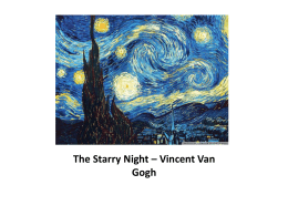
The Starry Night – Vincent Van Gogh
PowerPoint-Präsentation
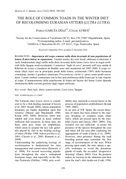
THE ROLE OF COMMON TOADS IN THE WINTER DIET OF
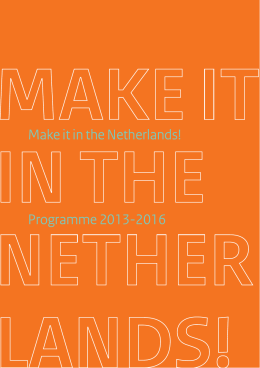
Make it in the Netherlands! Programme 2013-2016
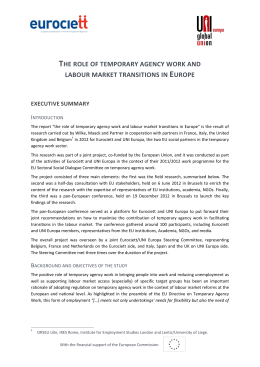
the role of temporary agency work and labour market