Keldysh Formalism: Non-equilibrium Green’s Function
Jinshan Wu∗
Department of Physics & Astronomy,
University of British Columbia,
Vancouver, B.C. Canada, V6T 1Z1
(Dated: November 28, 2005)
A review of Non-equilibrium Green’s Function (NEGF), also named as Keldysh Formalism, is
presented here. Perturbation theory is also builded up step by step on the basis of non-interacting
NEGF, and then leads to the Dyson’s Equation. Finally, application of NEGF on tight-binding
model with random impurity is explicitly calculated as an example.
I.
DEFINITION, FREE FIELD AND PERTURBATION
When only the properties of ground state is concerned, Zero-temperature (single- and many-particle) Green’s
function together with its perturbation theory principally gives all the information. Also if the equilibrium thermal
distribution is concerned, we can turn to Matsubara Green’s function and its perturbation theory[2]. However, we
may need to consider some more general states, such as a stationary non-equilibrium state – for example – a state
with nonzero current, or even an arbitrary state ρ, how to get correlation function for such system and then how to
do the corresponding perturbation expansion? In experiments of conductivity, there are such non-equilibrium system,
which has non-zero current and includes interaction between particles.
So in this note I will shortly review the idea and technics of Non-equilibrium Green’s function, also known as
Keldysh Formalism. All the formulas defined in this note is only for fermions, although it is not hard to make them
to also cover bosons.
Generally we need to calculate the Green’s function
³ n
o ´
i
†
G (x, t; x0 , t0 ) = − T r T ψH (x, t) ψH
(x0 , t0 ) ρH ,
(1)
~
where ψH (x, t) is the annihilation operator in Heisenberg picture, and ρ is the density matrix also in Heisenberg
picture. We will set ~ = 1 for a while. We also assume ρ is diagonal under particle number basis, [N, ρ] = 0. More
general density matrix could be possible, but not used anywhere yet.
For free field, this can be calculated quite strait forward, that
½
P
ψH (x, t) = k e−iω(k)t+ikx ck
P
,
(2)
†
ψH
(x, t) = k eiω(k)t−ikx c†k
then
P
0
0
G0 (x, t; x0 , t0 ) = −iθ (t − t0 ) k h1 − nk i e−iω(k)(t−t )+ik(x−x )
P
0
0
−iθ (t0 − t) k hnk i e−iω(k)(t−t )+ik(x−x )
(3)
Following the roadmap of zero-temperature Green’s function, next step would be to turn ψH (x, t) into interaction
picture ψI (x, t) and to somehow replace the real state ρH with state of non-interacting system ρ0H .
Let’s first organize the above mapping for zero-temperature Green’s function and then see if the same procedure
can be applied onto NEGF. Zero-temperature Green’s function is defined as a special case of eq(1), ρH = |Ωi hΩ|,
n
o
†
G (x, t; x0 , t0 ) = −i hΩ| T ψH (x, t) ψH
(x0 , t0 ) |Ωi ,
(4)
First, express T {AH (t1 ) BH (t2 )} in interaction picture.
H = H0 + e−²|t−t0 | H1 ,
(5)
AH (t) = eiH(t−t0 ) e−iH0 (t−t0 ) AI (t) eiH0 (t−t0 ) e−iH(t−t0 ) .
(6)
and
∗
[email protected]
2
−∞
∞
FIG. 1: The time-loop integration path.
Define unitary operator
U (t, t0 ) = eiH0 (t−t0 ) e−iH(t−t0 ) e−iH0 (t −t0 ) ,
(7)
∂
U (t, t0 ) = HI (t) U (t, t0 ) ,
∂t
(8)
0
which is the formal solution of
i
where HI (t) = eiH0 (t−t0 ) H1 e−iH0 (t−t0 ) . Or the explicit form is
U (t, t0 ) = T exp−i
Rt
t0
dtH I (t)
.
(9)
Then for t1 > t2 the time-ordered operators,
T {AH (t1 ) BH (t2 )} =
=
=
=
AH (t1 ) BH (t2 )
U † (t1 , t0 ) AI (t1 ) U (t1 , t0 ) U † (t2 , t0 ) BI (t2 ) U (t2 , t0 )
.
U (t0 , t1 ) AI (t1 ) U (t1 , t2 ) BI (t2 ) U (t2 , t0 )
U (t0 , ∞) U (∞, t1 ) AI (t1 ) U (t1 , t2 ) BI (t2 ) U (t2 , −∞) U (−∞, t0 )
(10)
Next for true ground state |Ωi, we can relate it with |0i, the ground state of non-interacting field,
U (t0 , −∞) |0i = lim eiH(−T −t0 ) e−iH0 (−T −t0 ) |0i = lim e−iH(T +t0 ) |0i .
T →∞
T →∞
(11)
According to Gell-Mann and Low Theorem, for adiabatic coupling, back in Schrödinger picture, ground state is stable,
|φ0 (tf )i ∝ U (tf , ti ) |φ0 (ti )i. In our case, |Ω (t0 )i ∝ U (t0 , −T ) |0 (−T )i, so up to some constant,
U (t0 , −∞) |0i ∝ |Ωi ⇒ U (−∞, t0 ) |Ωi ∝ |0i ,
(12)
and similarly, U (∞, t0 ) |Ωi ∝ |0i. Therefore, when t1 > t2
n
o
†
hΩ| T ψH (x, t) ψH
(x0 , t0 ) |Ωi ∝ h0| U (∞, t1 ) AI (t) U (t1 , t2 ) BI (t) U (t2 , −∞) |0i .
(13)
Finally, the constant can be eliminated as
G (x, t; x0 , t0 ) = −i
n
o
h0| T ψI (x, t) ψI† (x0 , t0 ) U (∞, −∞) |0i
h0| U (∞, −∞) |0i
,
(14)
where now all the quantities are from free field, and therefore can be calculated order by order by perturbation.
However, when we apply the same procedure to general ρH , we require the Gell-Mann and Low theorem holds for
excited states for both t = ±∞. This condition is too strong. The idea to solve above problem is to remove some
special points from the three special points t = (−∞, t0 , ∞), for example by setting t0 → ∞. In this way we require
that only |φ0 (−∞)i = |0i instead of both |φ0 (±∞)i = |0i. The path is to start along t = −∞ to t = t0 and then come
back along t = t0 to t = −∞. And finally let t0 → ∞, at pictured in fig(1). As inthe case of usual Green’s function,
let firstly reorganize T {A (t1 ) B (t2 )}, and then the relation between ρH and ρ0H . For t1 > t2 , insert U (−∞, ∞) into
eq(10),
T {AH (t1 ) BH (t2 )} = U (t0 , −∞) {U (−∞, ∞) U (∞, t1 ) AI (t1 )
U (t1 , t2 ) BI (t2 ) U (t2 , −∞)} U (−∞, t0 ) .
(15)
¯ ®
Then both sides relates only with U (−∞, t0 ), which still link the true eigenstates |ni with free-field eigenstates ¯n0 ,
that
¯ ®
U (−∞, t0 ) |ni ∝ ¯n0 .
(16)
3
t
t′
t′
t
(a) G+ (t, t′ ) and G− (t, t′ )
t
t′
t′
t
t′
t
−
(b) Gc (t, t′ )
−
t
t′
(c) G (t, t )
c̃
′
s
(d) Impurity Scattering
FIG. 2: One possible Feynman rules for NEGF.
Therefore, we arrive
G (x, t; x0 , t0 ) = −i
= −i
T r (U (−∞,∞)T {ψI (x,t)ψI† (x0 ,t0 )U (∞,−∞)}ρ0H )
T r (U (−∞,−∞)ρ0H )
T r (Tc {ψI (x,t)ψI† (x0 ,t0 )U (−∞,−∞)}ρ0H )
,
(17)
T r (U (−∞,−∞)ρ0H )
where Tc is the loop order as shown in fig(1) to order the time along the loop from −∞ to −∞. For example, at the
above branch it’s the same with time order Tc = T , while at the lower branch it’s anti-time order Tc = T̃ . And
U (−∞, −∞) = Tc exp−i
R −∞
−∞
dtH I (t)
.
(18)
One thing need to be noticed that in the final expression of Green’s function, all the time spots should be treated
as points at above branch (also call positive branch). However, later on, we will see that when we try to calculate
such Green’s function, we will need to do integral also over the lower branch (also call negative branch). This means
generally not all the time spots are at the positive branch, and the second line of eq(17) could not be separated as
U (−∞, ∞) and U (∞, −∞) outside and inside usual time order T . Therefore, generally we need to define Green’s
function according to the branches of t and t0 . There are four different configurations of them, as pictured in fig(2).
They are “less” and “greater” Green’s function[1],
³
´
³
n
¡
¢o´
†
G+ (x, t; x0 , t0 ) = −iT r ρH Tc ψH (x, t+ ) ψ † x0 , t0−
= iT r ρH ψH
(x0 , t0 ) ψH (x, t)
H
³
´ ,
³
n
(19)
¡
¢o´
†
0 0
G− (x, t; x0 , t0 ) = −iT r ρH Tc ψH (x, t− ) ψ † x0 , t0+
=
−iT
r
ρ
ψ
(x,
t)
ψ
(x
,
t
)
H
H
H
H
where t± means the time t is on positive/negative branch; “time ordered” and “anti-time ordered” Green’s function,
³
n
o´
³
n
¢o´
¡
†
0 0
Gc (x, t; x0 , t0 ) = −iT r ρH Tc ψH (x, t+ ) ψ † x0 , t0+
=
−iT
r
ρ
T
ψ
(x,
t)
ψ
(x
,
t
)
H
H
H
H
³
n
o´ ;
³
n
(20)
¡
¢o´
†
0 0
Gc̃ (x, t; x0 , t0 ) = −iT r ρH Tc ψH (x, t− ) ψ † x0 , t0−
=
−iT
r
ρ
T̃
ψ
(x,
t)
ψ
H
H
H (x , t )
H
4
and “retarded” and “advanced” Green’s function,
³ n
o´
Gr (x, t; x0 , t0 ) = −iθ (t − t0 ) T r ρH ψH (x, t) , ψ † (x0 , t0 )
H
³ n
o´ .
Ga (x, t; x0 , t0 ) = iθ (t0 − t) T r ρH ψH (x, t) , ψ † (x0 , t0 )
H
(21)
Only three of them are independent,
Gr = Gc − G+ = G− − Gc̃ , Ga = Gc − G− = G+ − Gc̃ .
This can be seen easily by separating G± as four parts, θ (t − t0 ) G± and θ (−t + t0 ) G± . Then
( c
G = θ (−t + t0 ) G+ + θ (t − t0 ) G−
Gc̃ = θ (t − t0 ) G+ + θ (−t + t0 ) G−
(22)
(23)
So Gc + Gc̃ = G+ + G− . Notice for “greater/less” Green’s function, different definitions and notations are used in
literature, for example, G> , G− and G< , G+ in [2]. Before we go further to perturbation calculation of interacting
field, let’s first list all the free-field Non-equilibrium Green’s functions.
P
0
0
G0,+ (x, t; x0 , t0 ) = i k hnk i e−iω(k)(t−t )+ik(x−x )
P
0
0
G0,− (x, t; x0 , t0 ) = −i k h1 − nk i e−iω(k)(t−t )+ik(x−x )
P
0
0
G0,c (x, t; x0 , t0 ) = −i k hθ (t − t0 ) − nk i e−iω(k)(t−t )+ik(x−x )
P
0
0
G0,c̃ (x, t; x0 , t0 ) = −i k hθ (t0 − t) − nk i e−iω(k)(t−t )+ik(x−x )
P
0
0
G0,r (x, t; x0 , t0 ) = iθ (t − t0 ) k e−iω(k)(t−t )+ik(x−x )
P −iω(k)(t−t0 )+ik(x−x0 )
G0,a (x, t; x0 , t0 ) = iθ (t0 − t)
e
(24)
k
About Eq(16), the expression similar with of Gell-Mann and Low Theorem, it should be understood in a kind
inverse logic order. For an interacting field H = H0 + H1 , the non-equilibrium density matrix ρH is not clearly
defined, while ρ0H of the corresponding free filed H0 could be well defined. Then the meaning of eq(16) is that we
start from ρ0H at t = −∞ and arrive a state at t = t0 , and then just use this new state as ρH . It’s not guaranteed
that this treatment will correspond to the true non-equilibrium distribution ρH . So for NEGF, even conceptually
instead of starting from the true ρH , we build up the theory from ρ0H . This could be a disadvantage of NEGF. Also
several advantages need to be noticed. First, this NEGF can be used for system at thermal equilibrium state, which
is usually the subject of Matsubara Green’s function. We will use as an example in §III. Second, even H1 explicitly
depends on t, this NEFG is still applicable, because we only set one end as H1 (−∞) = 0, H1 (∞) could be arbitrary.
At last, for non-equilibrium system as long as a unambiguous free-field corresponding non-equilibrium state could be
defined, we could always do the perturbation calculation order by order.
II.
SELF-ENERGY AND DYSON’S EQUATION
In order to arrive at the Dyson’s
P equation, we would firstly go to a little practice of first and second order calculation.
Consider an example with V = αβ Mαβ Cα† Cβ [2]. Then the first order perturbation gives,
XZ
¡ ©
ª¢
+
0
0,+
0
G (µ, t; ν, t ) = G (µ, t; ν, t ) −
dsMαβ T r Tc Cµ (t) Cν† (t0 ) Cα† (s) Cβ (s) .
(25)
αβ
The second term has one disconnected term and one non-zero connected term, which includes
©
ª® © † 0
ª®
P R
†
dsM
Tc Cν (t ) Cβ (s)
αβ Tc Cµ (t) Cα (s)
αβ
h
i
R∞
R −∞
P
= αβ −∞ dsG0,c (µ, t; α, s) Mαβ G0,+ (β, s; ν, t0 ) + ∞ dsG0,+ (µ, t; α, s) Mαβ G0,c̃ (β, s; ν, t0 )
(26)
At the next order, more terms will be coupled into this expansion series. Similarly G− also couples with all other
Gs. We will work out explicitly a special case of this interaction in the next section §III. Skipping some detailed
calculation here, overall these expansion series could be represented by a matrix equation, in the form of
³
´
(27)
Ĝ = Ĝ0 ΣĜ0 + Ĝ0 ΣĜ0 ΣĜ0 + · · · = Ĝ0 1 + ΣĜ
5
Like the example about disordered system in lecture notes[3], concept of self-energy Σ can be introduced. Then the
Dyson’s equation of NEGF could be organized as
ZZ ∞
0
0
0
Ĝ (t, t ) = Ĝ (t, t ) +
dt1 dt2 Ĝ0 (t, t1 ) Σ̂ (t1 , t2 ) Ĝ (t2 , t0 ) ,
(28)
−∞
where
µ
Ĝ =
Ĝc Ĝ−
Ĝ+ Ĝc̃
¶
,
(29)
and Ĝ (t, t0 ) is the operator form of G (x, t; x0 , t0 ) = hx| Ĝ (t, t0 ) |x0 i; Ĝ0 = D̂ is the free-field NEGF; and Σ̂ is the
self-energy term coming from interaction,
µ c
¶
Σ̂ Σ̂−
Σ̂ =
.
(30)
Σ̂+ Σ̂c̃
We will explain both theoretically and by examples how to get the self-energy term from interaction later. Let’s
temporally suppose they are known.
Because only three are independent of these six NEGFs, the above formula can be simplified further by choosing
the right three independent ones. Let’s use Ĝa , Ĝr and
F̂ = Ĝc + Ĝc̃ .
(31)
From eq(22) it is easy to see that this transformation is unitary,
¶
¶
µ
µ c
0 Ĝa
Ĝ Ĝ−
†
, Ǧ,
U
=
U
Ĝr F̂
Ĝ+ Ĝc̃
(32)
where
1
U=√
2
µ
1 −1
1 1
¶
.
Induced by this transformation, the self-energy term will transform as
¶
µ c
Σ̂ Σ̂−
U †,
Σ̌ , U
Σ̂+ Σ̂c̃
And finally, as we will see from the example in section §III, because generally Σc + Σc̃ = − (Σ+ + Σ− ),
¶
µ
Ω Σr
,
Σ̌ ,
Σa 0
(33)
(34)
(35)
Therefore, eq(28) still holds, but in a new form, or simply denoted as,
Ǧ = Ǧ0 + Ǧ0 Σ̌Ǧ.
(36)
Then the calculation of Green’s function becomes calculation of self-energy, where different approximations, such as
Born or Self-Consistent Born approximation, could be used.
III.
EXAMPLE
Let’s apply the general procedure above onto the following problem, the random impurity, a special case of the
example in section §II,
H=
X
k
² (k) Ck† Ck +
X M (q)
†
e−iq·X Ck+q
Ck ,
V
k,q,X
(37)
6
t
s
t
s
t′
t′
FIG. 3: First order expansion on loop path, LHS for s on positive branch, RHS for s on negative branch. Both of them are
zero if M (0) = 0.
s1
t
t′
s2
s1
t
s2
t′
FIG. 4: Second order expansion of G+ on loop path, for s1 , s2 both on positive branch.
with M (0) = 0 means average effect of impurity is zero. X is uniformly distributed so that k is still a good quantum
number, so G0 (k, t; k 0 , t0 ) = G0 (k, t; k, t0 ) δ (k − k 0 ) and G (k, t; k 0 , t0 ) = G (k, t; k, t0 ) δ (k − k 0 ). Let’s first work in time
domain, later on we will do the Fourier transformation to work in the frequency domain. First order expansion of
G+ , eq(26) for our special case will be
¸
Z −∞
X 1 ·Z ∞
0,c
0,+
0
0,+
0,c̃
0
dsG (k, t; k, s) M (0) G (k, s; k, t ) +
dsG (k, t; k, s) M (0) G (k, s; k, t ) = 0.
(38)
V
−∞
∞
X
Or equivalently by Feynman Diagram, as in fig(3). The second order expansion of G+ is,
ZZ
X
X
i
e−iq1 ·X1 −iq2 ·X2 M (q1 ) M (q2 ) ·
ds
ds
1
2
2V 2
C
k1 ,q1 ,X1 k2 ,q2 ,X2
³ n
o´,
† 0
†
†
T r Tc Ck (t) Ck (t ) Ck1 +q1 (s1 ) Ck1 (s1 ) Ck2 +q2 (s2 ) Ck2 (s2 )
(39)
where by Wick’s Theorem,
³ n
o´
T r Tc Ck (t) Ck† (t0 ) Ck†1 +q1 (s1 ) Ck1 (s1 ) Ck†2 +q2 (s2 ) Ck2 (s2 )
³ n
o´
³ n
o´
³ n
o´
= T r Tc Ck (t) Ck†2 +q2 (s2 ) T r Tc Ck1 (s1 ) Ck† (t0 ) T r Tc Ck2 (s2 ) Ck†1 +q1 (s1 ) .
³ n
o´
³ n
o´
³ n
o´
+T r Tc Ck (t) Ck†1 +q1 (s1 ) T r Tc Ck2 (s2 ) Ck† (t0 ) T r Tc Ck1 (s1 ) Ck†2 +q2 (s2 )
(40)
This has to be calculated for the four configurations of s1 , s2 . For example, here let’s work out for case of both s1 , s2
on positive branch.
ZZ ∞
X
i
2
ds
ds
|M (q1 )| e−iq1 ·X1 +iq1 ·X2 G0,c (k, t; k, s2 ) G0,+ (k, s1 ; k, t0 ) G0,c (k + q1 , s2 ; k + q1 , s1 )
1
2
2V 2
−∞
q1 ,X1 ,X2
ZZ ∞
X
i
2
ds1 ds2
|M (q2 )| eiq2 ·X1 −iq2 ·X2 G0,c (k, t; k, s1 ) G0,+ (k, s2 ; k, t0 ) G0,c (k + q2 , s1 ; k + q2 , s2 ). (41)
+ 2
2V
−∞
q2 ,X1 ,X2
ZZ ∞
X
i
2
= 2
ds1 ds2
|M (q)| eiq·X1 −iq·X2 G0,c (k, t; k, s1 ) G0,+ (k, s2 ; k, t0 ) G0,c (k + q, s1 ; k + q, s2 )
V
−∞
q,X1 ,X2
Those two term give the same contribution because of the integration and summation over s1 , s2 , q1,2 . Except that
here G+ couples with G0,c and etc, this expression has exactly the same form with the second order of the usual
7
G+
G−
Gc
Gc̃
Non-Zero Impurity Line
=
Σ1,c
Σ1,+
+...
Σ1,−
Σ1,c̃
FIG. 5: Another set of Feynman rules for NEGF, second order expansion is shown as example to express in these new rules.
Further perturbation could be done in this diagram form.
Green’s function with impurity. Similarly, G+ also coupled with G0,− , G0,c̃ and obviously G0,+ itself. So part of the
first order of self-energy term could be defined as
ZZ ∞ X
i
2
Σc (k; s2 , s1 ) ∝
|M (q1 )| e−iq1 ·X1 +iq1 ·X2 G0,c (k + q, s2 ; k + q, s1 ) .
(42)
2V 2
−∞
q1 ,X1 ,X2
So we get a term of G+ at the second order in the form of
G2,+ = G0,+ Σ1,c G0,c + . . .
(43)
If we check the term about G+ in eq(28), we will get
G2,+ = G0,+ Σ1,c G0,c + G0,c̃ Σ1,+ G0,c + G0,+ Σ1,− G0,+ + G0,c̃ Σ1,c̃ G0,+ ,
(44)
which does include the above term we already calculated. The diagram expression of all those four terms are shown in
the follow fig(5). A detail calculation include all the configuration of s1 , s2 will give us the left three terms. Similarly
we can do the second order expansion of G−,cc̃ . Then the third order expansion will give us more self-energy terms.
Finally, we can get the Dyson’s equation, which after Fourier transformation will lead us to frequency domain Dyson’s
equation.
In the Feynman diagrams in fig(2), where the time loop is explicitly down to be an indicator of the type of Green’s
function. Besides this, considering the character of our specific case, M (0) = 0, we may just use different lines to
represent different Green’s functions, so that the diagrams could be simpler, Here we skip the boring derivation of
eq(36), the matrix form Dyson’s equation, hopefully this will not stop one understanding the general picture of NEGF.
IV.
SUMMARY
Keldysh NEGF Formula is a generalization of the usual zero and non-zero temperature Green’s function. It can
be applied onto the usual equilibrium cases and non-equilibrium case. The way we derive such formula here is to
construct a loop from −∞ to ∞ and back to −∞, and introducing Green’s functions G (t, t0 ) corresponding to the
different configuration of (t, t0 ) over branches. Formally the structure of Green’s function and their Dyson’s Equation
8
looks equivalent with the one for usual Green’s Function. So all the perturbation calculation is quite straightforward.
However, in order to do the perturbation, a well-defined non-interacting state and Green’s function is a necessary
starting point. Whether such starting point leads to the real non-equilibrium state is questionable, and relies on the
comparison between calculation and experiments. There is another way to get this formula in [4], where the authors
use contour path over complex plan to replace above loop path. The derivation is more elegant in a sense, but the
problem of picking up the right starting point still exists, although the authors claim their treatment is exact more
or less.
[1] C. Caroli and R. Combrescot and P. Nozieres and D. Saint-James, Direct calculation of the tunneling current, J. Phys. C:
Solid St. Phys, 4(1971), 916-929.
[2] G. D. Manhan, Many-Particle Physics(1990 New York), Plenum Press.
[3] M. Berciu, Lecture notes for Phys503, 2005, http://www.physics.ubc.ca/∼berciu/ .
[4] H. Haug and A.P. Jauho, Quantum Kinetics in Transport and Optics of Semiconductors(1996 Berlin Heidelberg), SpringerVerlag.
Scarica