Examples
of
hybrid
MPC
©
2009
by
A.
Bemporad
Controllo
di
Processo
e
dei
Sistemi
di
Produzione
‐
A.a.
2008/09
1 /55
Hybrid
MPC
for
cruise
control
GOAL:
command
gear
ratio,
gas
pedal,
and
brakes
to
track
a
desired
speed
and
minimize
consumption
©
2009
by
A.
Bemporad
Controllo
di
Processo
e
dei
Sistemi
di
Produzione
‐
A.a.
2008/09
2 /55
Hybrid
Model
•
Vehicle
dynamics
=
vehicle
speed
=
traction
force
=
brake
force
discretized
with
sampling
time
•
Transmission
kinematics
ω =
engine
speed
M
=
engine
torque
i
=
gear
©
2009
by
A.
Bemporad
Controllo
di
Processo
e
dei
Sistemi
di
Produzione
‐
A.a.
2008/09
3 /55
Hybrid
Model
•
Engine
torque
•
Max
engine
torque
:
180
160
140
120
Piecewise‐linearization
(PWL
Toolbox,
Julián,
2000)
100
80
60
1000
2000
3000
4000
requires:
4
binary
aux
variables
4
continuous
aux
variables
(Note:
in
this
case
PWL
function
is
convex
)
could
be
handled
by
linear
constraints
without
introducing
any
binary
variable
!)
•
Min
engine
torque
©
2009
by
A.
Bemporad
Controllo
di
Processo
e
dei
Sistemi
di
Produzione
‐
A.a.
2008/09
4 /55
Hybrid
Model
•
Gear
selection:
for
each
gear
#i,
define
a
binary
input
•
Gear
selection
(traction
force):
depends
on
gear
#i
define
auxiliary
continuous
variables:
•
Gear
selection
(engine/vehicle
speed):
similarly,
also
requires
6
auxiliary
continuous
variables
©
2009
by
A.
Bemporad
Controllo
di
Processo
e
dei
Sistemi
di
Produzione
‐
A.a.
2008/09
5 /55
Hysdel
Model
go
to
demo
/demos/cruise/init.m
©
2009
by
A.
Bemporad
Controllo
di
Processo
e
dei
Sistemi
di
Produzione
‐
A.a.
2008/09
6 /55
Hybrid
Model
•
MLD
model
•
2
continuous
states:
x, v
(vehicle
position
and
speed)
•
2
continuous
inputs:
M,
Fb
(engine
torque,
brake
force)
(gears)
•
6
binary
inputs:
gR,
g1,
g2,
g3,
g4,
g5
(vehicle
speed)
•
1
continuous
output:
v
•
16
auxiliary
continuous
vars:
•
4
auxiliary
binary
vars:
(6
traction
force,
6
engine
speed,
4
PWL
max
engine
torque)
(PWL
max
engine
torque
breakpoints)
•
96
mixed‐integer
inequalities
©
2009
by
A.
Bemporad
Controllo
di
Processo
e
dei
Sistemi
di
Produzione
‐
A.a.
2008/09
7 /55
Hybrid
Controller
•
Max‐speed
controller
Objective:
maximize
speed
(to
reproduce
max
acceleration
plots)
250
200
MILP
optimization
problem
Linear
constraints
Continuous
variables
Binary
variables
Parameters
Time
to
solve
mp‐
MILP
(Sun
Ultra
10)
Number
of
regions
96
18
10
1
45
s
11
v(t)
150
100
50
0
x(t)
(x(t)
is
irrelevant)
(Parameters:
Renault
Clio
1.9
DTI
RXE)
©
2009
by
A.
Bemporad
Controllo
di
Processo
e
dei
Sistemi
di
Produzione
‐
A.a.
2008/09
8 /55
Hybrid
Controller
•
Max‐speed
controller
Velocity (km/h)
Gear
200
Fraction of Max Torque (Nm)
5
Brakes (Nm)
1
1
150
4
0.5
0.5
100
3
50
2
0
0
50
100
1
0
0
-0.5
-0.5
0
Road Slope (deg)
50
100
-1
0
Engine speed (rpm)
1
6000
50
100
0
Engine Torque (Nm)
200
50
100
Power (kW)
60
5000
50
0.5
150
4000
0
40
3000
100
30
2000
20
-0.5
50
1000
-1
-1
0
50
Time (s)
©
2009
by
A.
Bemporad
100
0
10
0
50
Time (s)
100
0
0
50
100
0
Time (s)
Controllo
di
Processo
e
dei
Sistemi
di
Produzione
‐
A.a.
2008/09
0
50
100
Time (s)
9 /55
Hybrid
Controller
•
Tracking
controller
250
MILP
optimization
problem
Linear
constraints
Continuous
variables
Binary
variables
Parameters
Time
to
solve
mp‐MILP
(PC
850Mhz)
Number
of
regions
98
19
10
2
200
vd(t)
43
s
49
150
100
50
0
go
to
demo
/demos/cruise/init_exp.m
©
2009
by
A.
Bemporad
0
40
Controllo
di
Processo
e
dei
Sistemi
di
Produzione
‐
A.a.
2008/09
80
120
v(t)
160
200
10 /55
Hybrid
Controller
•
Tracking
controller
Velocity (km/h), Desired velocity (km/h)
120
5
Gear
Brakes (Nm)
Fraction of Max Torque (Nm)
10000
1
100
8000
4
0.5
80
6000
60
3
0
4000
40
2
-0.5
2000
20
0
0
6
100
200
1
0
100
200
-1
0
6000
4
0
200
0
Engine Torque (Nm)
Engine speed (rpm)
Road Slope (deg)
100
100
200
Power (kW)
200
100
100
50
5000
2
4000
0
3000
-2
2000
0
0
-100
-4
-50
1000
-6
0
100
Time (s)
©
2009
by
A.
Bemporad
200
-200
0
0
100
Time (s)
200
-100
0
100
200
Time (s)
Controllo
di
Processo
e
dei
Sistemi
di
Produzione
‐
A.a.
2008/09
0
100
200
Time (s)
11 /55
Hybrid
Controller
•
Smoother
tracking
controller
250
MILP
optimization
problem
Linear
constraints
Continuous
variables
Binary
variables
Parameters
Time
to
solve
mp‐MILP
(PC
850Mhz)
Number
of
regions
100
19
10
2
47
s
54
200
150
vd(t)
100
50
0
0
40
80
120
160
200
v(t)
©
2009
by
A.
Bemporad
Controllo
di
Processo
e
dei
Sistemi
di
Produzione
‐
A.a.
2008/09
12 /55
Hybrid
Controller
•
Smoother
tracking
controller
Velocity (km/h), Desired velocity (km/h)
120
5
Gear
Brakes (Nm)
Fraction of Max Torque (Nm)
10000
1
100
8000
4
0.5
80
6000
60
3
0
4000
40
2
-0.5
2000
20
0
0
6
100
200
1
0
100
200
-1
0
6000
4
200
0
0
Engine Torque (Nm)
Engine speed (rpm)
Road Slope (deg)
100
100
200
Power (kW)
200
100
100
50
5000
2
4000
0
3000
-2
2000
0
0
-100
-4
-50
1000
-6
0
100
Time (s)
©
2009
by
A.
Bemporad
200
-200
0
0
100
Time (s)
200
-100
0
100
200
Time (s)
Controllo
di
Processo
e
dei
Sistemi
di
Produzione
‐
A.a.
2008/09
0
100
200
Time (s)
13 /55
Traction
Control
System
©
2009
by
A.
Bemporad
Controllo
di
Processo
e
dei
Sistemi
di
Produzione
‐
A.a.
2008/09
14 /55
Vehicle
Traction
Control
Improve
driver's
ability
to
control
a
vehicle
under
adverse
external
conditions
(wet
or
icy
roads)
Model
nonlinear,
uncertain,
constraints
Controller
suitable
for
real‐time
implementation
MLD
hybrid
framework
+
optimization‐based
control
strategy
©
2009
by
A.
Bemporad
Controllo
di
Processo
e
dei
Sistemi
di
Produzione
‐
A.a.
2008/09
15 /55
Tire
Force
Characteristics
©
2009
by
A.
Bemporad
Controllo
di
Processo
e
dei
Sistemi
di
Produzione
‐
A.a.
2008/09
16 /55
Simple
Traction
Model
(Borrelli,
Bemporad,
Fodor,
Hrovat,
2006)
•
Mechanical
system
•
Manifold/fueling
dynamics
•
Tire
torque
τt
is
a
function
of
slip
Δω and
road
surface
adhesion
coefficient
µ
wheel
slip
Δω
©
2009
by
A.
Bemporad
Controllo
di
Processo
e
dei
Sistemi
di
Produzione
‐
A.a.
2008/09
17 /55
Hybrid
model
Torque
Nonlinear
tire
torque
τt
=f(Δω ,
µ)
µ
Slip
PWA
Approximation
Torque
(PWL
Toolbox,
Julian,
2000)
µ
Mixed‐Logical
Slip
HYSDEL
Dynamical
(MLD)
Hybrid
Model
(discrete
time)
©
2009
by
A.
Bemporad
Controllo
di
Processo
e
dei
Sistemi
di
Produzione
‐
A.a.
2008/09
18 /55
MLD
model
State x ( t)
4
variables
Input u ( t)
1
variable
vars δ(
t)
1
variable
Aux.
Continuous
vars
z(t)
3
variables
Mixed‐integer
inequalities
14
Aux.
Binary
The
MLD
matrices
are
automatically
generated
in
Matlab
format
by
HYSDEL
go
to
demo
/demos/traction/init.m
©
2009
by
A.
Bemporad
Controllo
di
Processo
e
dei
Sistemi
di
Produzione
‐
A.a.
2008/09
19 /55
Performance
and
constraints
•
Control
objective:
•
Constraints:
•
Limits
on
the
engine
torque:
•
Note:
a
logic
constraint
(hysteresis)
may
be
also
taken
into
account
©
2009
by
A.
Bemporad
Controllo
di
Processo
e
dei
Sistemi
di
Produzione
‐
A.a.
2008/09
20 /55
Experimental
results
target speed
(250
ms
delay
from
commanded
to
actual
engine
torque
initial
overspin)
average driven
wheel speed
15
10
5
average
non-driven
wheel speed
0
Engine
Torque
Command,
[Nm]
controller is
triggered ON
Wheel
Speeds,
[rad/s]
20
200
150
100
50
0
0
3
6
9
12
6
Time,
[s]
9
12
Controller
Region
30
25
20
15
10
5
0
0
©
2009
by
A.
Bemporad
3
Controllo
di
Processo
e
dei
Sistemi
di
Produzione
‐
A.a.
2008/09
21 /55
Experiments
indoor
ice
arena
(µ¼
0.2)
2000
Ford
Focus
2.0l
4‐cyl
engine
5‐speed
manual
transmission
•
504
regions
•
20ms
sampling
time
•
Pentium
266Mhz
+
Labview
©
2009
by
A.
Bemporad
Controllo
di
Processo
e
dei
Sistemi
di
Produzione
‐
A.a.
2008/09
22 /55
Hybrid
Control
of
a
DISC
Engine
(Photo:
Courtesy
Mitsubishi)
(N.
Giorgetti,
G.
Ripaccioli,
Bemporad,
I.
Kolmanovsky
and
D.
Hrovat)
©
2009
by
A.
Bemporad
Controllo
di
Processo
e
dei
Sistemi
di
Produzione
‐
A.a.
2008/09
23 /55
DISC
engine
control
problem
Objective:
Develop
a
controller
for
a
Direct‐Injection
Stratified
Charge
(DISC)
engine
that:
•
Automatically
chooses
operating
mode
(homogeneous/stratified)
•
Can
cope
with
nonlinear
dynamics
Homogeneous
Stratified
•
Handles
constraints
(on
A/F
ratio,
air‐flow,
spark)
•
Achieves
optimal
performance
(tracking
of
desired
torque
and
A/F
ratio)
©
2009
by
A.
Bemporad
Controllo
di
Processo
e
dei
Sistemi
di
Produzione
‐
A.a.
2008/09
24 /55
DISC
engine
Two
distinct
regimes:
Regime
fuel
injection
air‐to‐fuel
ratio
Homogeneous
combustion
intake
stroke
λ=14.64
Stratified
combustion
compression
stroke
λ>14.64
•
Mode
is
switched
by
changing
fuel
injection
timing
(late
/
early)
•
Better
fuel
economy
during
stratified
mode
Periodical
cleaning
of
the
aftertreatment
system
needed
(λ=14.00,
homogeneous
regime)
normal
©
2009
by
A.
Bemporad
purge
the
stratified
operation
can
only
be
sustained
in
a
restricted
part
of
the
engine
operating
range
Controllo
di
Processo
e
dei
Sistemi
di
Produzione
‐
A.a.
2008/09
25 /55
DISC
engine
‐
States:
intake
manifold
pressure
(pm)
‐
Outputs:
Air‐to‐fuel
ratio
(λ),
torque
(τ),
max‐brake‐torque
spark
timing
(δmbt)
‐
Continuous
inputs:
spark
advance
(δ),
air
(Wth),
fuel
flow
(Wf)
flow
‐
Binary
input:
spark
combustion
regime
(ρ)
‐
Disturbance:
engine
speed
(ω)
[measured]
Constraints
on:
Air‐to‐fuel
ratio
(due
to
engine
roughness,
misfiring,
smoke
emiss.)
Spark
timing
(to
avoid
excessive
engine
roughness)
Mass
flow
rate
on
intake
manifold
(constraints
on
throttle)
• Dynamic
equations
are
nonlinear
• Dynamics
and
constraints
depend
on
regime
ρ
©
2009
by
A.
Bemporad
Controllo
di
Processo
e
dei
Sistemi
di
Produzione
‐
A.a.
2008/09
26 /55
DISC
dynamics
Nonlinear
model
of
the
engine
developed
(Kolmanovsky,
Sun,
…)
and
validated
at
Ford
Assumptions:
‐
no
EGR
(exhaust
gas
recirculation)
rate,
‐
engine
speed=2000
rpm.
•
Intake
manifold
pressure:
•
In‐cylinder
Air‐to‐Fuel
ratio:
•
Engine
torque:
with
functions
of
pm
where
θa,
θb,
δmbt
are
functions
of
λ,
δ
and
ρ
✓
Good
for
simulation
✖
Not
suitable
for
optimization‐based
controller
synthesis
©
2009
by
A.
Bemporad
Controllo
di
Processo
e
dei
Sistemi
di
Produzione
‐
A.a.
2008/09
27 /55
Hybridization
of
DISC
model
DYNAMICS
(intake
pressure,
air‐to‐fuel
ratio,
torque):
•
Definition
of
two
operating
points;
•
Linearization
of
nonlinear
dynamics;
•
Time
discretization
of
the
linear
models.
ρ‐dependent
dynamic
equations
CONSTRAINTS
on:
•
Air‐to‐Fuel
Ratio:
λmin(ρ)
·λ(t)
· λmax(ρ);
•
Mass
of
air
through
the
throttle:
0
·
Wth
·
K;
•
Spark
timing:
0
· δ(t)
· δmbt(λ,
ρ)
ρ−dependent
constraints
Hybrid
system
with
2
modes
(switching
affine
system)
©
2009
by
A.
Bemporad
Controllo
di
Processo
e
dei
Sistemi
di
Produzione
‐
A.a.
2008/09
28 /55
Integral
Action
Integrators
on
torque
error
and
air‐to‐fuel
ratio
error
are
added
to
obtain
zero
offsets
in
steady‐state:
=
sampling
time
brake
torque
and
air‐to‐fuel
references
Simulation
based
on
nonlinear
model
confirms
zero
offsets
in
steady‐state
(despite
the
model
mismatch)
©
2009
by
A.
Bemporad
Controllo
di
Processo
e
dei
Sistemi
di
Produzione
‐
A.a.
2008/09
29 /55
MPC
of
DISC
engine
N =
control
horizon
x(t)
=
current
state
where:
and:
Reference
values
are
automatically
generated
from
τref
and
λref
by
numerical
computations
based
on
the
nonlinear
model
©
2009
by
A.
Bemporad
Controllo
di
Processo
e
dei
Sistemi
di
Produzione
‐
A.a.
2008/09
30 /55
DISC
Engine
‐
HYSDEL
List
SYSTEM hysdisc{
INTERFACE{
STATE{
REAL pm
[1, 101.325];
REAL xtau
[-1e3, 1e3];
REAL xlam
[-1e3, 1e3];
REAL taud
[0,
100];
REAL lamd
[10,
60];
}
OUTPUT{
REAL lambda, tau, ddelta;
}
INPUT{
REAL Wth
[0,38.5218];
REAL Wf
[0,
2];
REAL delta
[0,
40];
BOOL rho;
}
PARAMETER{
REAL Ts, pm1, pm2;
…
}
}
taul={IF rho THEN tau11*pm+...
tau12*Wth+tau13*Wf+tau14*delta+tau1c
ELSE
tau01*pm+tau02*Wth...
+tau03*Wf+tau04*delta+tau0c };
dmbtl ={IF rho THEN dmbt11*pm+dmbt12*Wth...
+dmbt13*Wf+dmbt14*delta+dmbt1c+7
ELSE dmbt01*pm+dmbt02*Wth...
+dmbt03*Wf+dmbt04*delta+dmbt0c-1};
lmin ={IF rho THEN 13 ELSE 19};
lmax ={IF rho THEN 21 ELSE 38};
}
CONTINUOUS{
pm=pm1*pm+pm2*Wth;
xtau=xtau+Ts*(taud-taul);
xlam=xlam+Ts*(lamd-lam);
taud=taud; lamd=lamd;
}
OUTPUT{
lambda=lam-lamd;
tau=taul-taud;
ddelta=dmbtl-delta;
}
MUST{
lmin-lam
<=0;
lam-lmax
<=0;
delta-dmbtl <=0;
}
}
IMPLEMENTATION{
AUX{
REAL lam,taul,dmbtl,lmin,lmax;
}
DA{
lam={IF rho THEN l11*pm+l12*Wth...
+l13*Wf+l14*delta+l1c
ELSE
l01*pm+l02*Wth+l03*Wf...
+l04*delta+l0c
};
}
©
2009
by
A.
Bemporad
Controllo
di
Processo
e
dei
Sistemi
di
Produzione
‐
A.a.
2008/09
31 /55
MPC
‐
Torque
control
mode
Solve
MIQP
problem
(mixed‐integer
quadratic
program)
to
compute
u(t)
Weights:
(prevents
rρ unneeded
chattering)
pm
l
Wth
t
r
Wf
qτ
qλ
d
sετ
sελ
main emphasis on torque
©
2009
by
A.
Bemporad
Controllo
di
Processo
e
dei
Sistemi
di
Produzione
‐
A.a.
2008/09
MPC
32 /55
Simulation
Results
(nominal
engine
speed)
Time (s)
ω = 2000
rpm
Air‐to‐Fuel
Ratio
[Nm]
Engine
Brake
Torque
14
(Purge
Lean
NOx
Trap)
Time (s)
Time (s)
Combustion
mode
homogeneous
•
Control
horizon
N=1;
•
Sampling
time
Ts=10
ms;
•
PC
Xeon
2.8
GHz
+
Cplex
9.1
¼ 3
ms
per
time
step
stratified
Time (s)
©
2009
by
A.
Bemporad
Controllo
di
Processo
e
dei
Sistemi
di
Produzione
‐
A.a.
2008/09
33 /55
Simulation
Results
(varying
engine
speed)
Air‐to‐Fuel
Ratio
[Nm]
Engine
Brake
Torque
Time (s)
Time (s)
Engine
speed
20
s
segment
of
the
European
drive
cycle
(NEDC)
Hybrid
MPC
design
is
quite
robust
with
respect
to
engine
speed
variations
Time (s)
©
2009
by
A.
Bemporad
Controllo
di
Processo
e
dei
Sistemi
di
Produzione
‐
A.a.
2008/09
34 /55
Simulation
Results
(varying
engine
speed)
Air‐to‐Fuel
Ratio
[Nm]
Engine
Brake
Torque
Time
Time (s)
(s)
Engine
speed
20
s
segment
of
the
European
drive
cycle
(NEDC)
Hybrid
MPC
design
is
quite
robust
with
respect
to
engine
speed
variations
rpm
4
Nm
Time (s)
Control
code
too
complex
(MILP)
!
not
implementable
!
©
2009
by
A.
Bemporad
Time (s)
Controllo
di
Processo
e
dei
Sistemi
di
Produzione
‐
A.a.
2008/09
35 /55
Explicit
MPC
Controller
Explicit
control
law:
N=1
(control
horizon)
42
partitions
where:
•
Time
to
compute
explicit
MPC:
¼
3s;
Cross‐section
by
the
τref‐λref
plane
•
Sampling
time
Ts=10
ms;
•
PC
Xeon
2.8
GHz
+
Cplex
9.1
ρ=0
! 8
µs
per
time
step
¼ 3ms
on
ρ=1
©
2009
by
A.
Bemporad
µ−controller
Motorola
MPC
555
43kb
RAM
(custom
made
for
Ford)
Controllo
di
Processo
e
dei
Sistemi
di
Produzione
‐
A.a.
2008/09
36 /55
Explicit
MPC
Controller
(N=2)
Explicit
control
law:
N=2
(control
horizon)
747
partitions
where:
Engine
Brake
Torque
Closed‐loop
N=2
©
2009
by
A.
Bemporad
Air‐to‐Fuel
Ratio
Closed‐loop
N=1
Controllo
di
Processo
e
dei
Sistemi
di
Produzione
‐
A.a.
2008/09
Adequate
!
37 /55
Explicit
Hybrid
MPC
of
Semiactive
Suspensions
(joint
work
with
N.
Giorgetti,
H.E.
Tseng,
D.
Hrovat)
©
2009
by
A.
Bemporad
Controllo
di
Processo
e
dei
Sistemi
di
Produzione
‐
A.a.
2008/09
38 /55
Quest
of
Optimal
Semi‐Active
Suspensions
Ms=suspended
mass
Mus=unsprung
mass
x4
sprung
mass
velocity
suspension
deflection
x2
unsprung
mass
velocity
tire
deflection
For
Semi‐Active
with
Variable
Damping,
f(x)=C*(x4‐x2)
Cmax
Clipped
Optimal
Cmin
C=f(x)/(x4‐x2),
where
f(x)
is
the
optimal
active
suspension
force
C=sat[f(x)/(x4‐x2)]
Optimal
©
2009
by
A.
Bemporad
?
=
Controllo
di
Processo
e
dei
Sistemi
di
Produzione
‐
A.a.
2008/09
39 /55
Quest
of
Optimal
Semi‐Active
Suspensions
Showed
existence
by
posing
as
two
point
boundary
problem,
Hrovat,
Margolis,
and
Hubbard,
1988.
Showed
the
optimal
solution
can
be
solved
from
three
Riccati
Equations
(state
dependent
switching),
Butsuen
and
Hedrick,
1989.
Showed
the
optimal
solution
(of
unsaturated
component)
maintains
a
‘linear’
(varying
gain)
feedback
form,
Tseng
and
Hedrick,
1994.
Showed
Clipped
Optimal
cannot
be
the
optimal
through
a
counter
example,
Tseng
and
Hedrick,
1994.
Does
Closed
Loop
Form
Optimal
Solution
Exist?
N.
Giorgetti,
A.
Bemporad,
H.
E.
Tseng,
and
D.
Hrovat,
“Hybrid
model
predictive
control
application
towards
optimal
semi‐active
suspension,”
International
Journal
of
Control,
vol.
79,
no.
5,
pp.
521–533,
2006.
©
2009
by
A.
Bemporad
Controllo
di
Processo
e
dei
Sistemi
di
Produzione
‐
A.a.
2008/09
40 /55
Sub‐Optimal
SA
Suspensions
Steepest
Gradient
(SGM):
“Improve
the
action
of
a
passive
suspension”
Shock
test
of
initial
condition
SGM
16%
better
than
clipped‐LQR
Clipped‐LQR
is
at
least
16%
from
the
true
optimal
©
2009
by
A.
Bemporad
Controllo
di
Processo
e
dei
Sistemi
di
Produzione
‐
A.a.
2008/09
41 /55
Semiactive
Suspensions
suspension
deflection
tire
deflection
Quarter‐car
model
linear
model
f-
Constraints:
1)
Passivity
condition:
no
ok
2)
Max
dissipation
power:
ok
no
x4‐x2
3)
Saturation:
(1),
(2)
are
nonlinear
&
nonconvex
physical
constraints
©
2009
by
A.
Bemporad
Hybrid
Model
Controllo
di
Processo
e
dei
Sistemi
di
Produzione
‐
A.a.
2008/09
42 /55
Model
•
State‐space
model
•
Output:
•
Cost:
J=
=
!
!
(qx1 x21 + qx3 x23 + ẋ24 )dt
(x! Qx + ẋ24 )dt
•
Time‐discretization:
©
2009
by
A.
Bemporad
Controllo
di
Processo
e
dei
Sistemi
di
Produzione
‐
A.a.
2008/09
43 /55
Constraints
1)
Passivity
condition:
fno
ok
ok
no
x4‐x2
2)
Max
dissipation
power:
where
3)
Saturation:
©
2009
by
A.
Bemporad
Controllo
di
Processo
e
dei
Sistemi
di
Produzione
‐
A.a.
2008/09
44 /55
HYSDEL
Model
/* Semiactive suspension system
(C) 2003-2005 by A.Bemporad, D.Hrovat,
E.Tseng, N.Giorgetti
*/
SYSTEM suspension {
INTERFACE {
STATE {
REAL x1 [-0.05,0.05];
REAL x2 [-5,5];
REAL x3 [-0.2,0.2];
REAL x4 [-2,2];
}
INPUT{
REAL u [-10,10]; /* m/s^2 */
}
OUTPUT {
REAL y;
}
PARAMETER {
REAL A1dot,A2dot,A3dot,A4dot,B4dot,ws;
REAL A11,A12,A13,A14,B1,A21,A22,A23,A24,B2;
REAL A31,A32,A33,A34,B3,A41,A42,A43,A44,B4;
}
}
IMPLEMENTATION {
AUX {
BOOL sign;
BOOL usign;
REAL F;
}
AD {
sign = x4-x2<=0;
usign = u<=0;
}
DA {
F={ IF sign THEN u-(2*25.5*ws)*(x4-x2)
ELSE -u+(2*25.5*ws)*(x4-x2)};
}
OUTPUT {
y=A1dot*x1+A2dot*x2+A3dot*x3
+A4dot*x4+B4dot*u;
}
CONTINUOUS {
x1 = A11*x1+A12*x2+A13*x3+A14*x4+B1*u;
x2 = A21*x1+A22*x2+A23*x3+A24*x4+B2*u;
x3 = A31*x1+A32*x2+A33*x3+A34*x4+B3*u;
x4 = A41*x1+A42*x2+A43*x3+A44*x4+B4*u;
}
MUST {
sign -> usign;
~sign -> ~usign;
F>=0;
} } }
>>S=mld('semiact3',Ts)
get
the
MLD
model
in
Matlab
>>[X,T,D,Z,Y]=sim(S,x0,U);
simulate
the
MLD
model
©
2009
by
A.
Bemporad
Controllo
di
Processo
e
dei
Sistemi
di
Produzione
‐
A.a.
2008/09
45 /55
Hybrid
PWA
Model
•
PWA
model
•
4
continuous
states
•
1
continuous
input
•
2
polyhedral
regions
>>P=pwa(S);
©
2009
by
A.
Bemporad
Controllo
di
Processo
e
dei
Sistemi
di
Produzione
‐
A.a.
2008/09
46 /55
Simulation
in
Simulink
©
2009
by
A.
Bemporad
Controllo
di
Processo
e
dei
Sistemi
di
Produzione
‐
A.a.
2008/09
47 /55
Control
Strategy:
MPC
past
future
Predicted
outputs
y(t+k|t)
Manipulated
Inputs
u(t+k)
t t+1
Model
Predictive
(MPC)
Control
t+T
•
At
time
t
solve
with
respect
to
the
finite‐horizon
open‐loop,
optimal
control
problem:
•
Apply
(first
optimal
control
move)
and
discard
the
remaining
optimal
inputs);
•
Repeat
the
whole
optimization
at
time
t+1
©
2009
by
A.
Bemporad
Controllo
di
Processo
e
dei
Sistemi
di
Produzione
‐
A.a.
2008/09
48 /55
Performance
Specs
tire deflession
suspension
deflession
vertical
acceleration
terminal weight
(Riccati matrix)
©
2009
by
A.
Bemporad
Controllo
di
Processo
e
dei
Sistemi
di
Produzione
‐
A.a.
2008/09
49 /55
Hybrid
MPC
‐
Example
>>refs.y=1;
% weights output #1
>>Q.y=Ts*rx4d;% output weight
…
>>Q.norm=2;
% quadratic costs
>>N=1;
% optimization horizon
>>limits.umin=umin;
>>limits.umax=umax;
>>C=hybcon(S,Q,N,limits,refs);
>> C
Hybrid controller based on MLD model S <semiact3.hys> [2-norm]
4
1
1
4
0
state measurement(s)
output reference(s)
input reference(s)
state reference(s)
reference(s) on auxiliary continuous z-variables
4 optimization variable(s) (2 continuous, 2 binary)
13 mixed-integer linear inequalities
sampling time = 0.01, MIQP solver = 'cplex'
Type "struct(C)" for more details.
>>
>>[XX,UU,DD,ZZ,TT]=sim(C,S,r,x0,Tstop);
©
2009
by
A.
Bemporad
Controllo
di
Processo
e
dei
Sistemi
di
Produzione
‐
A.a.
2008/09
50 /55
Closed‐loop
MPC
in
Simulink
©
2009
by
A.
Bemporad
Controllo
di
Processo
e
dei
Sistemi
di
Produzione
‐
A.a.
2008/09
51 /55
Explicit
Hybrid
MPC
>>E=expcon(C,range,options);
>> E
Explicit controller (based on hybrid controller C)
4 parameter(s)
1 input(s)
8 partition(s)
sampling time = 0.01
The controller is for hybrid systems (tracking)
[2-norm]
This is a state-feedback controller.
Type "struct(E)" for more details.
>>
Section
in
the
(x3,x4)‐space
for
x1=x2=0
©
2009
by
A.
Bemporad
Controllo
di
Processo
e
dei
Sistemi
di
Produzione
‐
A.a.
2008/09
52 /55
Explicit
Hybrid
MPC
Generated
C‐code
©
2009
by
A.
Bemporad
Controllo
di
Processo
e
dei
Sistemi
di
Produzione
‐
A.a.
2008/09
53 /55
Quest
of
Optimal
Semi‐Active
Suspensions
©
2009
by
A.
Bemporad
Controllo
di
Processo
e
dei
Sistemi
di
Produzione
‐
A.a.
2008/09
54 /55
Simulation
Results
•
Horizon
N=1:
same
as
Clipped‐LQR
!
•
For
increasing
N:
better
closed‐loop
performance
Explicit
solution
(N=1,
x1=x2=0):
Performance
Index
N=1,
Same
Cost
Value
!
•
Simulations
with
road
noise.
•
Initial
condition
x(0)=[0
0
0
0]’
•
Simulation
time
T=20
s,
sampling
time
Ts=10
ms
©
2009
by
A.
Bemporad
Controllo
di
Processo
e
dei
Sistemi
di
Produzione
‐
A.a.
2008/09
55 /55
Scarica